

Abstract
A new cell-vortex unstructured finite volume method for structural dynamics is assessed for simulations of structural dynamics in response to fluid motions. A robust implicit dual-time stepping method is employed to obtain time accurate solutions. The resulting system of algebraic equations is matrix-free and allows solid elements to include structure thickness, inertia, and structural stresses for accurate predictions of structural responses and stress distributions. The method is coupled with a fluid dynamics solver for fluid-structure interaction, providing a viable alternative to the finite element method for structural dynamics calculations. A mesh sensitivity test indicates that the finite volume method is at least of second-order accuracy. The method is validated by the problem of vortex-induced vibration of an elastic plate with different initial conditions and material properties. The results are in good agreement with existing numerical data and analytical solutions. The method is then applied to simulate a channel flow with an elastic wall. The effects of wall inertia and structural stresses on the fluid flow are investigated.
Keywords: finite volume method, structural dynamics, vortex-induced plate vibration, channel flow with elastic walls
1. Introduction
In terms of numerical simulation, the finite element (FE) method is the most popular tool for computational structural dynamics (CSD) problems, whereas traditionally the finite volume (FV) method is widely used in computational fluid dynamics (CFD). Both techniques solve the integral governing equations by means of weighted residual methods where they differ in the selected weighting functions. The FV method may be considered as a particular case of the FE method with non-Galerkin weighting [1]. However, their different properties, applications, and directions of development have resulted in numerical software tools for CFD and CSD that are different in almost every aspect. The efforts to bridge the differences between them have been attempted. In particular, Bathe et al. [2–5] proposed a flow-condition-based interpolation (FCBI) finite element scheme for incompressible fluid flows to achieve local mass and momentum conservation which was considered the unique property of the FV method. The FCBI finite element procedure was applied to solve multi-physics problems in a consistent FE framework and its accuracy was assessed by the goal-oriented error estimation technique [6, 7]. The current effort also attempts to bridge the gap between FE and FV by developing an unstructured-grid FV structural dynamic solver and by integrating the structural solver with a baseline fluid solver for fluid-structure interaction (FSI) simulation. The proposed method in this work can assist FV-based CFD researchers with applying FV-based structural dynamics for FSI problems.
Generally speaking, the essential difference between FE and FV in the numerical discretization of second-order partial differential equations is negligible and for many cases the two methods are almost equivalent [8]. In recent years, the FV methods have been applied to a number of problems in various aspects of CSD. For example, the plate bending analysis has been performed using FV methods by Demirtzic et al. [9], Wheel [10], and Fallah [11]; the solutions of different solid mechanics problems [12, 13], the stress analysis of elasto-plastic solids by Demirtzic et al. [14], the analysis of dynamic solid mechanics [15], and the application to FSI by Slone et al. [16] have also been reported. These works prove that for CSD problems the FV methods are competitive with the FE methods in terms of numerical accuracy and computational efficiency. Wheel [17] even showed that the FV method achieves greater accuracy than the FE method for a benchmark problem in selected test cases. The implementation of FV methods for CSD computations can be classified into two categories: the cell-centered approach [9, 10, 12, 14, 17] and the cell-vertex approach [1, 13, 15, 16, 18]. Both approaches are locally and globally conservative. In the cell-vertex approach, the displacement and stress variables are stored at the vertices of the mesh which are themselves enclosed by control volumes formed by the median duals of the mesh. In the cell-centered approach, the variables are stored at the centroids of cells which are also used as control volumes themselves. Thus the cell-vertex approach needs considerably less computational effort and memory for a given mesh. And the cell-vertex approach is better suited to compute stresses, especially when the meshes become highly skewed; it is therefore chosen in this work to develop the structural solver. With the implementation of FV methods for structural dynamics, the numerical solutions satisfy both local and global conservations. And unlike other FV methods, the cell-vertex FV method employed in this work does not use shape functions for spatial discretizations and it is the matrix-free, thus reducing the computational efforts and storage requirements.
The FSI simulation has recently been an intensively researched area of CFD and CSD. It has widespread applications in diverse fields such as deformation of artificial lung [6], analyses of industrial applications [19], aeroelastic analysis [16, 20], wind response of buildings and structures [21], blood flow in veins and arteries [22–24], heart valves dynamics [25], and airflow in collapsible airways [26]. However, an accurate and efficient computational model for this problem still poses a great challenge, which is often aggravated by large deformations and complex geometries of the closely coupled fluid-structure system. Various strategies and numerical methods have been developed towards solving the FSI problems in different areas. They can be categorized into two categories: the Eulerian method and the arbitrary Lagrangian Eulerian (ALE) method. In the Eulerian method, the fluid flow is computed on a stationary mesh and the mesh update is avoided, which makes it more efficient and easy to implement. However they suffer some accuracy problems in the interpolation of fluid variables near the FSI interface. The ALE method uses body-fitted meshes and does remeshing as the fluid-structure interface moves, which generally results in higher accuracy though requiring more computational efforts on mesh treatment. In recent years, different ALE methods have been developed and widely used in various areas, such as airflow past the parachute [27], flow past a flapping wing [28], transient motion of a missile [29], stokes flow in an elastic tube [30], and among others. In this work, we adopt a dynamic mesh based ALE method to couple the FV structural dynamics solver with the fluid dynamics solver.
The objective of the work is to assess the accuracy of a new cell-vertex unstructured finite volume method for structural dynamics in response to fluid motions. The goal is to provide an alternative approach to the FE method for the analysis of structural dynamics in dealing with FSI problems. In the current method, the structure domain is discretized into an unstructured grid for complex geometries. The stresses are calculated in a cell-by-cell manner based on a cell-based data structure and stress distribution is linear within cells, but can be discontinuous across different cells, even within the same control volume. The control volumes are constructed around vertices using the median dual of the grid. The deformation gradients and stresses are evaluated using Green’s Theorem. Time-accurate solutions are obtained by employing an implicit dual time stepping scheme, wherein a pseudo time term is added to the dynamic structural equations and the physical time term is integrated by a second-order backward time discretization scheme and the pseudo time term is finally eliminated by a sub-iteration process. For the fluid domain, the governing incompressible Navier-Stokes equations are spatially discretized on an unstructured grid, which is solved by the implicit characteristic-Galerkin approximation together with the fractional four-step algorithm [31]. At the fluid structure interface, the two meshes conform to each other for the implementation of the ALE algorithm. To handle the motion of the fluid mesh, an efficient dynamic mesh algorithm [32] is adopted. The fluid-structure coupling is achieved in an interactive manner, in which both the fluid and structure governing equations are computed separately depending on the exchange of boundary conditions at the fluid-structure interface.
The paper is laid out as follows. In section 2, the governing equations and FV formulation for structural dynamics are introduced. Numerical techniques for solving the governing equations are also outlined. In section 3, the governing equations for fluid dynamics and the associated computational methodologies are briefly described. In section 4, the implementation of the dynamic mesh method and the solution procedure for the FSI is presented. In section 5, some benchmark cases are presented for estimation of the order of accuracy of the scheme and validation of the model. The coupled FSI system is then applied to study the effects of wall inertia and structural stresses on the fluid flow in a channel flow with an elastic wall.
2. Finite Volume Formulation for Structural Dynamics
2.1 Governing Equation
The governing equation for a continuum undergoing motion is given by the Cauchy’s equation:
| (1) |
where b is the body force, σij is the stress tensor, ρ is the material density, and a is the acceleration. For the structure considered here, the body force is negligible compared with stresses and other forces acting on them. There are two major types of forces: damping and external forces. External forces generally vary as functions of time. Damping is the ability of a structure to dissipate energy. In structural mechanics, the most common damping device is the ideal linear viscous damper. For a structure with linear viscous damping, the damping is directly proportional to the structure velocity, while acting in the opposite direction of the velocity. Discarding the body force and considering the influences of external and damping forces, Eq. (1) becomes
| (2) |
where f is the external force, U is the structure velocity, and c is the damping ratio. The only external force considered here is the fluid force acting at the fluid-structure interface, which can be incorporated through the boundary conditions. Thus the external force term in Eq. (2) is omitted hereafter. For a detailed description about force equilibrium, please refer to Bathe [33].
2.2 Constitutive Relationship and Displacement Formulation
The constitutive relationship between stress and strain is the generalized Hook’s law. For an isotropic homogeneous structure, it is given as
| (3) |
where E is the Young’s Modulus, and υ is the Poisson’s ratio of the structure. The stress vector is σT = [σxx σyy τxy] and the strain vector is εT = [εxx εyy γxy]. The elastic strain can also be expressed in terms of total and initial strains σ = D(εt - ε0), where D is the constitutive matrix as expressed in Eq. (3), and εt and ε0 are the total and initial strains, respectively.
To allow large nonlinear deformation, the Green-Lagrange tensor is adopted to describe the strain-displacement relationship.
| (4) |
where di is the displacement tensor. In two-dimensional (2D) vector form d = (dx,dy), Eq. (4) reads
| (5) |
where L is the matrix of differential operators. Substitution of the constitutive stress-strain Eq. (3) and the strain-displacement Eq. (5) to the dynamic equilibrium Eq. (2) yields
| (6) |
which is subject to the boundary conditions:
| (7) |
Here the structural boundary is the union of the prescribed displacement boundary dp and the prescribed traction boundary tp which includes the external force f. T is the matrix of outward normal operators.
| (8) |
where n = (nx, ny) is the unit vector outward normal to the domain boundary.
2.3 Spatial Discretization
Equation (6) is discretized on an unstructured triangular grid and a cell-vertex scheme is adopted to construct control volumes [34]. The spatial discretization is performed by using the integral form of the conservation equations over the control volume surrounding node P shown in Fig. 1.
| (9) |
The first term on the left-hand side of Eq. (9) is converted to a line integral via the divergence theorem of Gauss and, and is then approximated by
| (10) |
where ncell is the number of triangular cells associated with node P, Δlci is the part of control volume boundary in cell Ci, and Δlpi is the edge vector of cell Ci that is opposite to vertex P. Here the value (DLd - Dε0)i is calculated at the center of the triangular cell Ci, which can be obtained by using Green’s theorem based on the variables at the three vertices of the triangle. Like the Galerkin type of formulation, the gradient of a flow variable ø at the center of a triangle is evaluated by
| (11) |
where øi is the flow variable at vertex i of a triangular cell, Δli is the edge vector facing node i, and A is the area of the triangle.
Fig. 1.
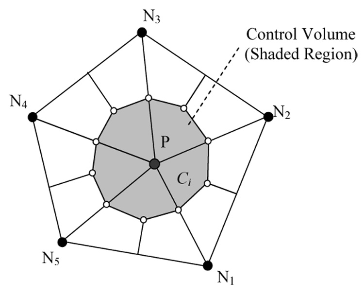
Construction of the control volume for node P.
2.4 Temporal Discretization and Integration
The time dependent term is discretized using an implicit second-order accurate backward differencing scheme. To achieve matrix-free operation and to use a larger time step size, a dual time-stepping scheme [35] is adopted by adding a pseudo time derivative term to Eq. (6). Re-writing the integral equation Eq. (9) for a given node P together with Eq. (10) yields
| (12) |
where the superscript n denotes the real time level. Then the solution is sought by marching Eq. (12) in τ to a pseudo steady state. We adopt a five-stage Runge-Kutta scheme for pseudo time integration for stability and convergence.
| (13) |
where the superscript m denotes the pseudo time level and the coefficients for the five-stage Runge-Kutta time integration are as follows:
The five-stage time integration scheme is of 4th-order accuracy and allows a large time step, but it is also computationally expensive. It is noteworthy that Bathe [36] proposed a two-step implicit time integration scheme for transient FE solutions of structural dynamics. The first step is based upon delta-form Newmark scheme with a half time step, and the second step utilizes the three-point backward Euler scheme as in Eq. (12). Although the scheme requires twice the computational effort of Newmark scheme, it achieved better energy and momentum conservation and is more stable.
The cell-vertex FV method does not use shape functions for spatial discretization and it is matrix-free, thus reducing the computational efforts and storage requirements. Of particular note is the structural dynamics solver that can treat a structure of finite thickness so that all components of the structural stress can be obtained.
After the velocity is obtained, the displacement is calculated using the second-order backward difference scheme:
| (14) |
So
| (15) |
3. Mathematical Formulation for the Fluid
The governing Navier-Stokes equations for the incompressible viscous flow in the ALE framework for FSI read:
| (16) |
| (17) |
where ui, p, ν and ρ are the fluid velocity, pressure, kinematic viscosity, and density, respectively. is velocity of the fluid mesh and represents the ALE convective velocity induced by the difference between the fluid velocity and the mesh velocity.
The ALE modified governing equations are solved by using a fractional four-step method [31]. In this method, an intermediate velocity is first obtained from the momentum Eq. (16) with the pressure gradient calculated from the old pressure field. As a result, there is no need for special treatment of the velocity boundary condition. However, the intermediate velocity does not necessarily satisfy the continuity equation, so a new pressure field is calculated by solving a pressure-Poisson equation which is derived by enforcing the continuity constraint Eq. (17). The velocity is then corrected by the updated pressure to satisfy Eq. (17). The equations in the four-step method are solved by the implicit characteristic Galerkin approximation. The fluid solver is second-order accurate in both time and space [31].
4. Dynamic Mesh Method and Coupling Algorithm
Mesh movement is handled by using a dynamic mesh method [32]. In this method, the shortest distance d(is) of every fluid node (is) to the moving or solid walls is calculated and the wall node closest to this inner node is identified (iswall). This distance d(is) is non-dimensionalized by the maximum value dmax of all the d(is). The deformation of the fluid node is calculated as the product of a distance function f(is) and the deformation of its associated wall node :
| (18) |
The distant function is constructed using two exponential damping functions as:
| (19) |
where
The distance function Eq. (19) approaches 1 when d goes to 0 and the function approaches 0 when d goes to dmax. This property makes the grid very rigid in areas near the wall and far away the wall while those in between areas are elastic and easy to be deformed. To make this method more robust for large mesh deformation, the calculated deformation of every node is further smoothed to eliminate highly skewed or overlapping cells. The smoothing is done by averaging the deformation of node k with the deformation of its neighboring nodes.
| (20) |
where nedge(k) is the number of edges surrounding node k. ki is the inverse of the distance from node k to edge i. The mesh velocities of the inner fluid nodes are obtained in the same way as the deformation.
The current coupled FSI system is treated as a triple-domain problem that includes the fluid domain, the structure domain, and the moving mesh. The relationship of these three domains is depicted in Fig. 2. The FSI coupled equations are solved in an iterative manner, which is shown in the flow chart of Fig. 3. The Navier-Stokes equations are solved first for the fluid domain. The solutions of the fluid provide external forces including fluid pressure and shear stress to the structure domain. The dynamics equation is then solved for the structure under the influences of fluid forces, which provides deformation and velocity boundary conditions at the fluid-structure interface. The fluid mesh is moved by the dynamic mesh algorithm in accordance with these boundary conditions, which updates the mesh deformation and ALE velocity for the computation of fluid domain for the next time step.
Fig. 2.
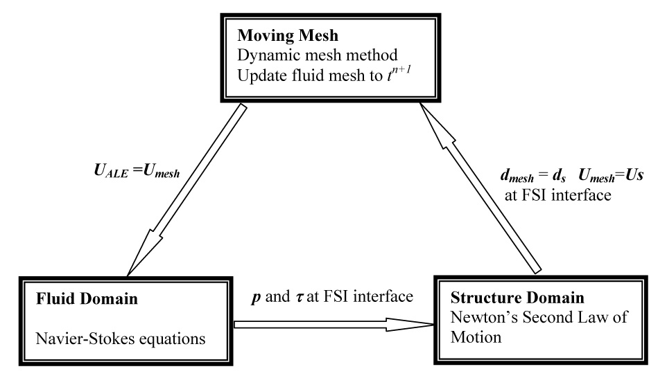
The relationship between the fluid and structure domains.
Fig. 3.
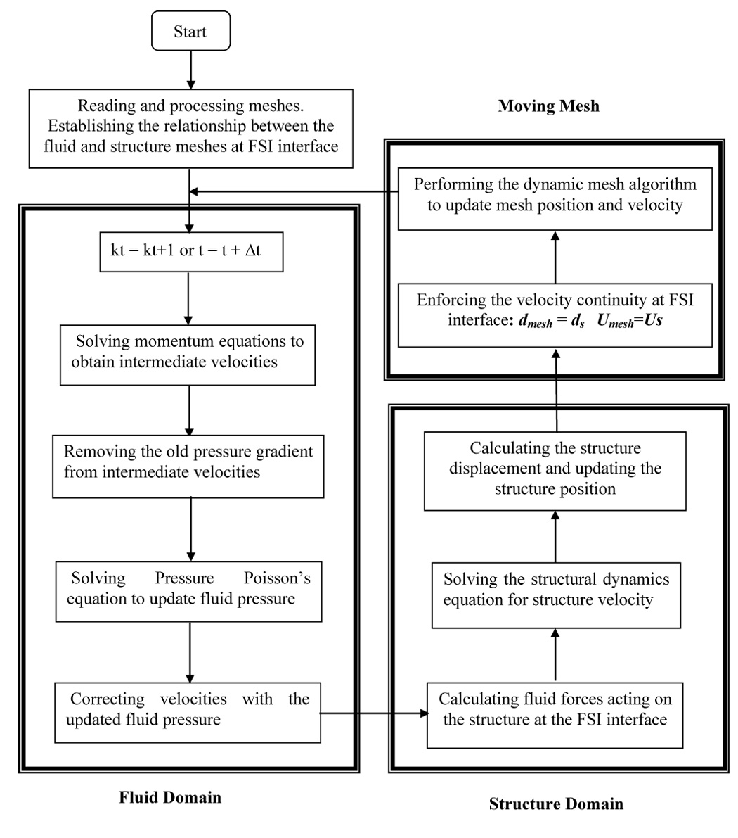
Flow chart of the fluid-structure interaction solution procedure.
Through the ALE and dynamic mesh method, the cell-vertex unstructured FV method for structural dynamics can be integrated with the fluid dynamics solver for FSI problems. The coupling system does not impose any ad hoc assumptions on the fluid, structure or moving mesh domains, which is critical to achieve a realistic representation of the physical reality of any system.
5. Computational Results
In this section, a grid convergence study is first performed for accuracy assessment of FV-based spatial discretization. Then the problem of vortex-induced vibration of an elastic plate is examined for model validation. Finally a channel flow with an elastic wall of different wall thickness is simulated to study the effects of wall inertia and structural stresses on the flow pattern.
5.1 Grid convergence study and error analysis
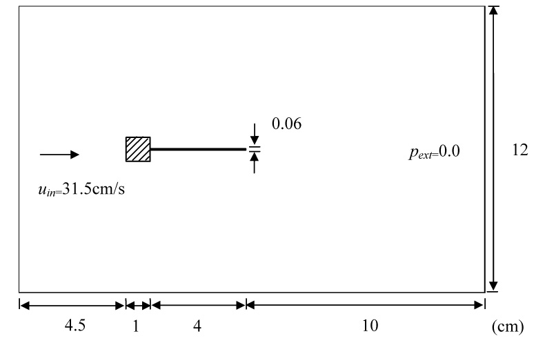
To verify the implementation of fluid-structure interaction algorithm and assess the accuracy of the FV method for structural dynamics, a grid convergence study is performed for a case where a flexible plate is situated at the center of a 2D channel as depicted in Fig. 4. The width and length of the channel are 2cm and 20cm, respectively, while the width and length of the flexible plate are 0.2cm and 1.6cm, respectively. Table 1 lists the properties of the fluid and the plate. Solid wall conditions are applied at the upper and lower boundaries of the channel, and stress free conditions are assumed at the outlet. A sinusoidal velocity uin = 1.5 sin(2πt) with a period T = 1s is applied at the inlet. The maximum inlet velocity is 1.5cm/s, so the maximum Reynolds number of the flow is 300. Four levels of consecutively finer meshes are used for simulation. For each mesh, both structure and fluid domains are discretized with a uniform grid distance h, and the grid distance of a finer mesh is a half of that of its next coarser mesh as shown in Fig 5. The meshes for the plate are constructed in a way that every node on the coarser meshes coincide with that of the finest mesh, i.e. the reference mesh, to avoid interpolations when comparing the solutions on different meshes. The grid distance and the number of nodes are listed in Table 2. A time step size of 0.01s is used.
Fig. 4.
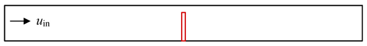
Model used for error analysis.
Table 1.
Properties of fluid and structure used for the grid convergence study
| Fluid Properties | Structure Properties | ||
|---|---|---|---|
| Density ρf (g·cm−3) | 1.0 | Density ρs (g·cm−3) | 1.0 |
| Viscosity µ (g·cm−1s−1) | 1.0×10⁻² | Poisson’s ratio |
0.49 |
| Young’s modulus E ( g·cm−1s−2) | 5.0×10⁴ | ||
Fig. 5.
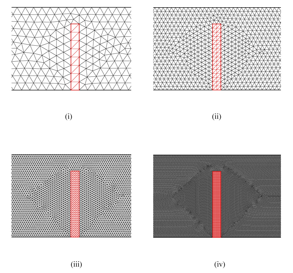
Four consecutively finer meshes used for grid independence study and error analysis.
Table 2.
Grid convergence study.
| Mesh | (i) | (ii) | (iii) | (iv) | |
|---|---|---|---|---|---|
| Grid distance | 0.2 cm | 0.1 cm | 0.05 cm | 0.025 cm | |
| Number of elements | fluid | 2,299 | 8,838 | 35,956 | 142,110 |
| structure | 16 | 64 | 256 | 1,024 | |
| Tip displacement | 0.082cm | 0.126cm | 0.158cm | 0.163cm | |
| λ calculated from L1 | 2.24 | ||||
| λ calculated from L2 | 2.30 | ||||
| λ calculated from L∞ | 2.01 | ||||
With the pulsatile inflow, the flexible plate deflects back and forth in the direction of the fluid flow. The solver runs 10T for the plate to achieve its stable vibration status. Then the solutions are recorded at T/4 when the plate is at its maximum deflection in the flow direction as presented in Fig. 6. The tip displacements of the plate at this moment are summarized in Table 2. It is observed that the solution obtained on mesh (iii) is very close to that obtained on mesh (iv), indicating the coupled solver is grid independent. Since there is no analytical solution to the system, the solution obtained on the finest mesh (iv) is treated as the “exact” solution and is used as a basis in calculation of the errors of the coarser solutions. The errors are calculated for the displacements dx of the plate. For a mesh of n nodes, the kth error norm and the infinity error norm of dx with respect to the “exact” solution (dx)e are calculated as follows,
| (21) |
The convergence history of L1, L2, and L∞ error norms for the three coarser meshes with respect to the finest mesh are shown in Fig. 7 against the grid distance h in a log-log manner. In the plot, the convergence rates of L1 and L2 are higher than slope 2. The overall slope for L∞ is smaller than those of L1 and L2, but it is still very close to 2. To further analyze the accuracy of the solver, the Richardson formula is used to estimate the order of accuracy of the coupled system.
| (22) |
where fj denotes the numerical solution obtained on the jth mesh, and ‖ ‖ represents any of the error norms L1, L2, and L∞. The computation for γ is performed on meshes (ii), (iii), and (iv). The results are summarized in Table 2. All the computed values of γ are greater than 2, which indicates that the current cell-vertex unstructured FV method for structural dynamics is at least second-order accurate.
Fig. 6.
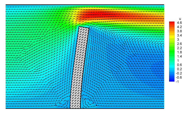
The flow field at T/4 obtained from mesh (iii).
Fig. 7.
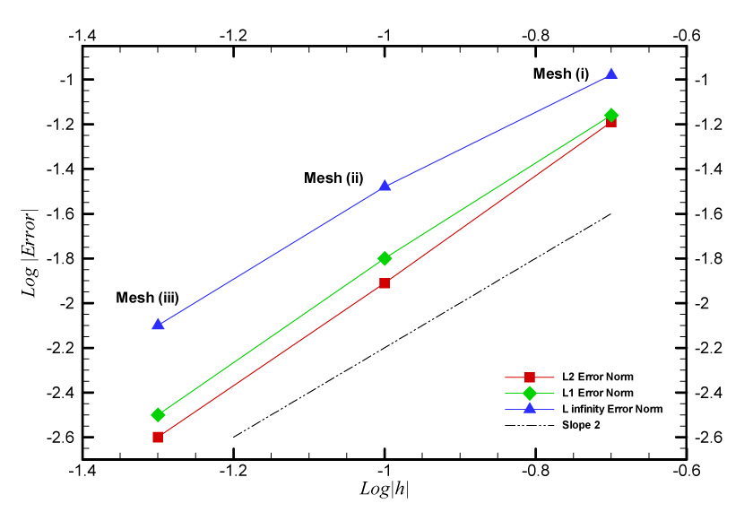
Convergence history of the error norms.
5.2 Flow-induced vibration of an elastic plate
In this problem, an elastic plate is attached to a rigid square cylinder at the center of its downstream face as shown in Fig. 8. This example was proposed by Wall et al. [37], and many other researchers like Dettmer et al. [38], Hübner et al. [39] and Teixeira et al. [40] also studied this model to test their numerical methods for the FSI problems. A uniform and constant velocity uin is imposed at the inlet, and the outlet pressure pout is set to 0. The no-slip boundary condition is applied to all the solid walls. The elastic plate is fully clamped into the square cylinder, which means:
d = 0, no displacement occurs at the fixed end;
∇d = 0, rotation of the fixed end is suppressed;
Q ≠ 0, shear forces are calculated;
M ≠ 0, bending moments are calculated.
Fig. 8.
Geometry of the model for vortex-induced vibration of an elastic plate.
The material properties for both the fluid flow and the plate are listed in Table 3, which are chosen to be consistent with those used by Hübner [39]. Since the vibration frequency of plate is higher than the first natural frequency of the plate of 0.61Hz, the structural damping is not considered here. The inflow velocity uin is set to 31.5cm/s, so the Reynolds number is 204, whereby L is the width of the square rigid body.
Table 3.
Material properties of the fluid flow and the elastic plate
| Fluid Properties | Structure Properties | ||
|---|---|---|---|
| Density ρf (g·cm−3) | 1.18×10⁻³ | Density ρs (g·cm−3) | 2.0 |
| Viscosity µ (g·cm−1s−1) | 1.82×10⁻⁴ | Poisson’s ratio |
0.35 |
| Young’s Modulus E (g·cm−1s−2) | 2.0×10⁶ | ||
Both fluid and structure domains are discretized into unstructured triangular meshes as shown in Fig. 9(a). The fluid mesh is of 4,319 nodes and the structure mesh is of 41×4 nodes. At the fluid-structure interface, the two set of meshes conform to each other as seen in the close-up view of the meshes in Fig. 9(b). A time step size of 0.001s is used in the simulation. In each physical time steps, 200 sub-iterations are used for pseudo-time stepping in the structure domain in order to achieve divergence-free conditions. The order of the residual is 10−6.
Fig. 9.
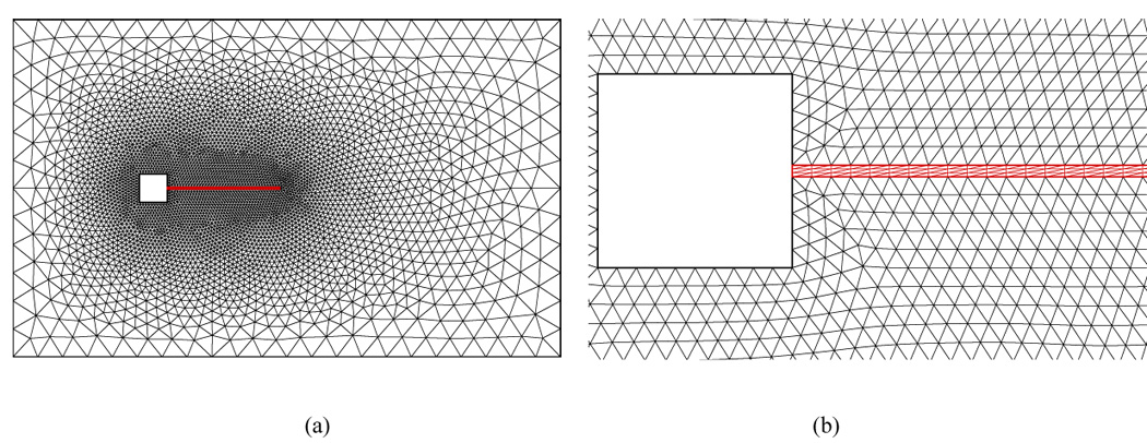
(a) unstructured mesh for the fluid domain (b) close-up view of the mesh near the plate.
Initially, a very large Young’s modulus is assumed to harden and fix the plate to obtain a fully developed flow around the rigid square cylinder. In the fully developed flow as presented in Fig. 10, vortices are shed from the corners of the square cylinder periodically with a frequency of 3.6Hz, as indicated in the variance of fluid forces in Fig. 11. This frequency is very close to the frequency of 3.7Hz reported in [39]. It is observed that within each shedding period three vortices move along the fixed plate, with two small vortices on one side and one large vortex on the other side as shown in Fig. 10. This distribution pattern of vortices induces pressure imbalance around the plate and causes the plate to vibrate when the Young’s modulus is reduced.
Fig. 10.
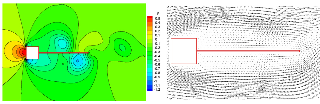
Pressure contour and velocity vector of the fluid flow with a fixed plate.
Fig. 11.

Variance of fluid forces acting on the fixed plate.
After t ≥ 10s when the fluid flow is fully developed, the Young’s modulus is reduced to E=2.0×10⁶ g·cm−1s−2, allowing drastic interaction between the flow and the elastic plate. The elastic plate starts to vibrate under the influence of the fluid force induced by vortex shedding. Two examples of the deformed fluid meshes are presented in Fig. 12. No excessively skewed or distorted cells are observed in the deformed meshes even when the structure deformation is relatively large, proving the robustness of the dynamic mesh method. Fig. 13 shows the time history of the tip displacement of the plate. It is found that the vibration amplitude of the plate increases gradually until the elastic plate finally reaches a stable vibration status with an amplitude of 0.81cm and a frequency of 3.3Hz, which agree well with Hübner’s simulation results [39]. Several snapshots of the fluid flow of 3/4 vibration period are presented in Fig. 14. The fluid flow with the vibrating plate is quite different from the one with the fixed plate, in which only one primary vortex exists along the plate. The primary vortex appears alternately on each side of the plate during a vibration period, and it is always located on the side opposite to the moving direction of the plate. In contrast, for the flow over a fixed plate the vortices move along the both sides of the plate simultaneously. When the elastic plate starts to move towards one side, the vortices on this side are weakened and eventually suppressed by the fluid motion associated with the plate vibration. However, the vortices on the opposite side are strengthened and enlarged by the fluid motion, producing only one large vortex on this side. The vortex eventually separates from the plate near the free end and produces a small vortex rotating in the opposite direction as shown in Fig. 14(b), which causes disturbances of the resulting fluid forces as presented in Fig. 15. It is also observed in Fig. 15 that the resulting fluid forces have a phase angle of about 180° with the plate vibration, where was also reported in [39]. Comparing Fig. 11 and Fig. 15, it is found that the resulting fluid forces on the vibrating plate are much larger than those on the fixed plate. It is because the structure motions strengthen the vortex on one side and weaken the one on the other side of the plate, thus increasing the pressure imbalance around the plate and producing larger resulting fluid forces.
Fig. 12.
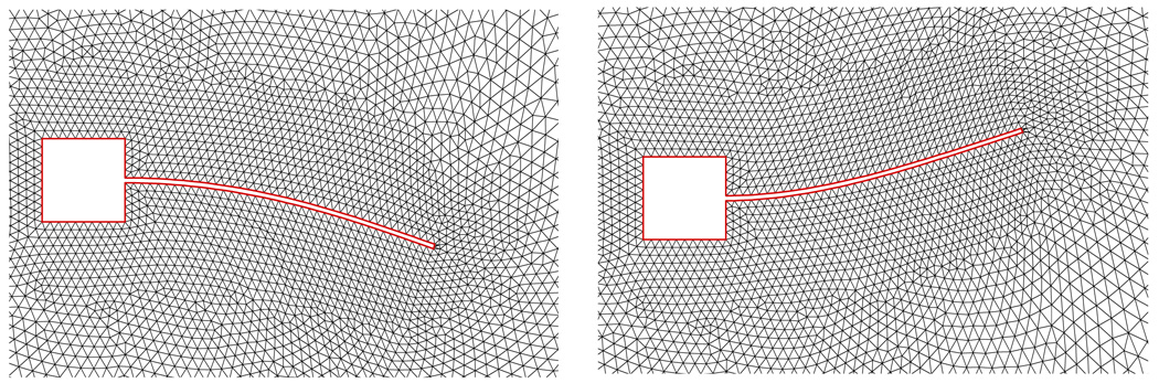
Deformed meshes.
Fig. 13.

Time history of the tip displacement of the elastic plate.
Fig. 14.
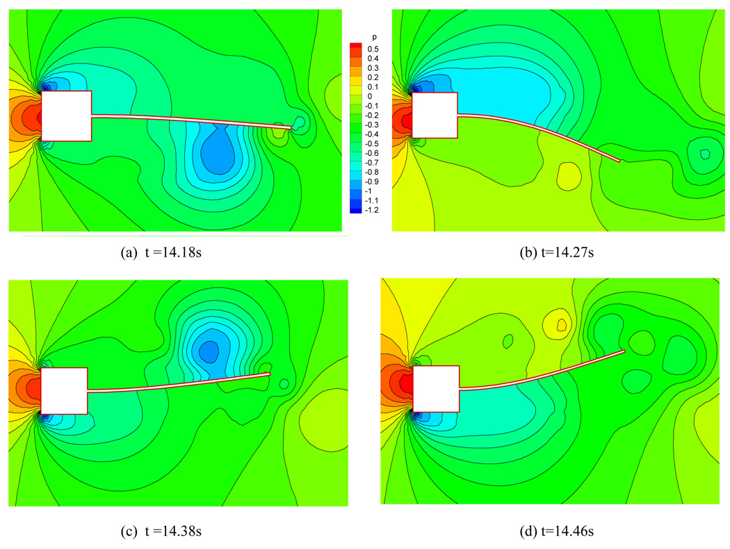
Pressure contours of the fluid flow with an elastic plate.
Fig. 15.

Time history of the tip displacement and fluid force.
Stress distributions in the thin elastic plate at t=14.46s are presented in Fig. 16. The stress distributions are compared with the analytical solutions of the same clamped-free end plate with the same extent of displacement under a constant load (without ambient fluid). At t=14.46s, the tip displacement of plate Dy is 0.81cm. For a clamped-free end beam with the geometry of l (length)×h (height)×w (width), a load of should be imposed at the free end to achieve the same extent of displacement [41]. The maximum bending stress per unit width at the root occurs at the lower surface of the beam and is calculated as follows:
| (23) |
Fig. 16.

Distributions of stresses σxx τxy and σyy at t=14.46s (unit: g·cm−1·s−2).
With the F load, the maximum bending stress at the root of the beam is 9,625 g·cm−1·s−2. In the calculated results shown in Fig. 16, the bending stress on the lower surface at the root of beam registers a value of 9,810 g·cm−1·s−2, about 1.9% deviation from the analytical result of 9,625 g·cm−1·s−2. The distribution of shear stress in the beam has a parabolic shape along the transverse direction, having a maximum shear stress at the center and zero values on the upper and lower surfaces [41]. The maximum shear stress per unit width is calculated as
| (24) |
The maximum shear stress at the center is 32 g·cm−1·s−2 in the simulated result, which agrees with the analytical solution of 34 g·cm−1·s−2 calculated by Eq. (24).
It is found that with an initial displacement, the behavior of the plate changes greatly. A temporary load is imposed on the elastic plate first to obtain an initial tip displacement Dy=0.78cm and then the load is released. Unlike the one with no initial displacement, the elastic plate reaches its stable vibration status very quickly as seen in Fig. 17. The frequency of the vibration also decreases to 2.0 Hz. It indicates that the dynamic interplay between an elastic plate and the fluid flow is strongly dependent on the initial conditions.
Fig. 17.

Time history of the tip displacement of the plate with initial displacement Dy=0.78cm.
With different material properties, the plate can develop different modes of vibration. By reducing the Young’s modulus to E=1.0×10⁶ g·cm−1·s−2, the plate develops the second mode of vibration as demonstrated by the time history of the tip displacement in Fig. 18. But with a stiffer material property, the plate can sustain the fluid forces with smaller or even no displacement as in the case of the flow with a fixed plate. Even with an initial deformation, the vibration of a stiffer plate is eventually subdued as presented in Fig. 19, the displacement history of an elastic plate with E=8.0×10⁶ g·cm−1·s−2.
Fig. 18.

Time history of the tip displacement of the elastic plate with E = 1.0×10⁶ (g·cm−1s−2).
Fig. 19.

Time history of the tip displacement of the elastic plate with E = 8.0×10⁶ (g·cm−1s−2).
All the simulations in this work are run on a HP xw9300 workstation with dual processors of 2.4GHz and a memory size of 8GB. The CPU time of the above simulations varies between 150–200 minutes.
5.3 Unsteady flow in a 2D channel with a flexible wall
The problem of fluid flow in a channel with elastic walls is of great importance for many biological systems, and has been widely studied in the last several decades. However due to the complicated interaction between the fluid flow and the channel wall, this problem is still not well understood. The early studies had been focused on one-dimensional (1D) models of these systems, which mainly investigated the flow limitation, self-excitation, and wave propagation. And analyses of these 1D models were based on many special assumptions, which limited their capabilities to investigate the complex FSI. 2D models were developed recently to provide a more realistic representation of the system, including Zhao et al. [32], Heil [42], Luo et al. [43, 44] and Rugonyi and Bathe [45]. In their models, the Navier-Stokes equations for the fluid were solved simultaneously with shell theory for the elastic wall. Shell theory is usually used for the thin-walled structure where the wall thickness is small compared with other dimensions. However, for moderate wall thickness, the solid element of finite thickness is more appropriate for the computation. And with this type of solid element, detailed stress distributions can be obtained to provide more insights into the structural responses.
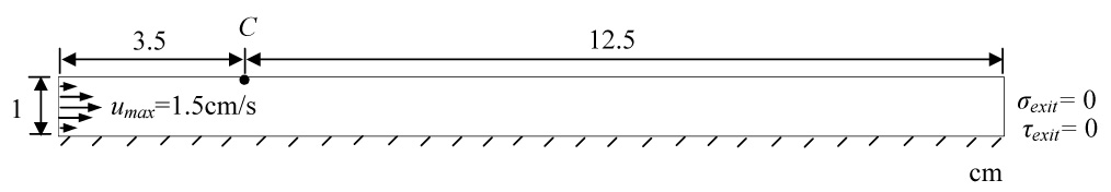
Here a 2D channel with a flexible wall of finite thickness is computed to investigate the unsteady flow in a channel in response to large deformation of the channel wall. The channel configuration is illustrated in Fig. 20. The width of the channel is D=1cm and the length is 16D. The upper wall is elastic and a control point C is placed at 3.5D away from the inlet to record the displacement history of the flexible wall.
Fig. 20.
A 2D channel with a flexible wall.
The channel flow with flexible walls is very complex and sensitive to the problem boundary conditions and the material properties of the walls, see the analysis in [42–44]. The undisturbed Poiseuille flow with average velocity of u0 =1.0 cm/s is assumed at the inlet and the stress free conditions are imposed at the outlet. The no-slip condition is applied to the lower solid wall. The density and viscosity of the fluid are 1.0 g·cm−3 and 2.0×10⁻³ g·cm−1s−1, respectively, so the Reynolds number of the flow is 500. The thickness of the channel wall is t=0.05D, while the Young’s modulus of the wall is E=5.2×10⁵ (g·cm−1s−2) and the Poisson’s ratio is set to 0. The density of the wall is 1.0 g·cm−3, so the structure-fluid mass ratio is 0.05. The flexible wall is fully clamped at both inlet and outlet ends. The fluid mesh has 6,074 nodes and the structure mesh has 1,152 (=4×288) nodes. A close-up view of the mesh near the structure is displayed in Fig. 21. The simulation is performed with a physical time step size of 0.002s. In each physical time steps, 200 sub-iterations are used to achieve divergence-free conditions with the residual order of 10−6. The CPU time for this simulation is 218 minutes for 10 periodic cycles on a HP xw 9300 workstation.
Fig. 21.

Close-up view of the mesh near the flexible wall.
The time history of displacement at control point C is presented in Fig. 22. At the early stage of the flow, with the sudden increase of the inlet velocity, a pressure wave propagates through the channel. Under the influence of fluid forces, the wall deforms with a relatively large displacement. The flexible wall bulges outwards and acts like a buffer to the fluid flow as shown in Fig. 23(a). However the internal stress of the flexible wall soon reduces the extreme deformation to moderate values after t ≥ 2s. And after t ≥ 6.5s, the fluid flow and the wall develop a stable periodic response as shown in Fig. 22. The distributions of the structural stresses of the flexible wall at t=7.27s are shown in Fig. 24. It can be seen that the maximum values of all the stresses are more than 102 Pa and all the stress components are within comparable ranges, so none of the stress components is negligible at this thickness-width ratio (t/D=1/20), proving that the solid elements are more suitable than the shell elements for a wall of finite thickness. To investigate the influences of the wall thickness and inertia to the fluid flow and structure responses, another case with a wall thickness of t=0.1D is studied. While all the other conditions remain the same, the structure-fluid mass ratio is set to 0.1. With a larger wall thickness and inertia, the deformation of the wall decreases. The maximum deformation is 0.18cm, while it is 0.3cm for the thinner wall. The fluid flow and the wall still develop a stable periodic response. However the system achieves the stable status at 0.8s, much faster than the thinner wall due to larger structure internal stresses associated with the thicker wall. The stress distributions are similar with those of the thinner wall, but with larger values. The maximum bending stress σxx is 1.2×10⁴ g·cm−1·s−2, and the maximum τxy and σyy are 7.5×10³ and 2.0×10³ g·cm−1·s−2, respectively. It is noteworthy that the shear stress τxy and the normal stress σxy are more significant in the thicker wall, which are definitely non-negligible. The two cases exhibit quite different features due to different wall thickness, thus it is important to take into account the effects of wall thickness and inertia in studying the channel flow with a flexible wall, e.g. blood flow and pulmonary flow
Fig. 22.

Time history of the displacement at control point C.
Fig. 23.

Pressure contours of the channel flow.
Fig. 24.

Distributions of stresses σxx τxy and σyy at t=7.27s (unit: g·cm−1·s−2)
6. Conclusions
A time-accurate cell-vertex unstructured finite volume method for structural dynamics in response to fluid motions is examined for assessment of accuracy, model validation, and its capabilities of handling structural responses. The method is integrated with a fluid dynamics solver through a dynamic mesh algorithm and the ALE method for fluid-structure interaction problems. A grid sensitivity test indicates that the method is at least second-order accurate. For model validation, the coupled FSI system is applied to simulate the vortex-induced vibration of an elastic plate, whose results agree well with the analytical solutions and other published results of the same test case. The results further show that different vibration modes of the plate may develop due to variation in material properties. For the channel flow with an elastic wall, it is observed that the self-excited oscillation develops under the influence of the fluid forces. The oscillation exhibits a long-term periodic response having a large amplitude at the early stage of the flow development. The wall thickness and inertia can influence the fluid-structure interaction and structural responses, thus they should be taken into account in the analysis of channel flow with flexible walls. This works demonstrates that the cell-vertex unstructured finite volume method may serve as a viable alternative to the finite element method for the analysis of structural dynamics.
Acknowledgements
This work was supported by a National Institutes of Health grant R01-EB-005823 awarded through the National Institute for Biomedical Imaging and Bioengineering under the IMAG program for Multiscale Modeling.
Footnotes
Publisher's Disclaimer: This is a PDF file of an unedited manuscript that has been accepted for publication. As a service to our customers we are providing this early version of the manuscript. The manuscript will undergo copyediting, typesetting, and review of the resulting proof before it is published in its final citable form. Please note that during the production process errors may be discovered which could affect the content, and all legal disclaimers that apply to the journal pertain.
Reference
- 1.Onate E, Cevera M, Zienkiewicz OC. A finite volume method format for structural mechanics. Inter J of Numer Methods in Eng. 1994;37:181–201. [Google Scholar]
- 2.Bathe KJ, Zhang H. A Flow-Condition-Based interpolation finite element procedure for incompressible fluid flows. Comput Struct. 2002;80:1267–1277. [Google Scholar]
- 3.Kohno H, Bathe KJ. A Flow-Condition-Based interpolation finite element procedure for triangular grids. Inter J of Numer Methods in Fluids. 2005;49:849–875. [Google Scholar]
- 4.Kohno H, Bathe KJ. Insight into the Flow-Condition-Based interpolation finite element approach: solution of steady-state advection-diffusion problems. Inter J of Numer Methods in Eng. 2005;63:197–217. [Google Scholar]
- 5.Kohno H, Bathe KJ. A 9-node quadrilateral FCBI element for incompressible Navier-Stokes flows. Comm in Numer Methods in Eng. 2006;22:917–931. [Google Scholar]
- 6.Bathe KJ, Zhang H. Finite element developments for general fluid flows with structural interactions. Inter J of Numer Methods in Eng. 2004;60:213–232. [Google Scholar]
- 7.Grätsch T, Bathe KJ. Goal-oriented error estimation in the analysis of fluid flows with structural interactions. Comput Methods Appl Mech Eng. 2006;195:5673–5684. [Google Scholar]
- 8.Idelsohn SR, Onate E. Finite volumes and finite elements: two ‘Good Friends’. Inter J of Numer Methods in Eng. 1994;37:3323–3341. [Google Scholar]
- 9.Demirdzic I, Muzaferija S, Peric M. Benchmark solutions of some structural analysis roblems using finite volume method and multigrid acceleration. Inter J of Numer Methods in Eng. 1997;40:1893–1908. [Google Scholar]
- 10.Wheel MA. A finite volume method for analysing the bending deformation of thick and thin plates. Comput Methods Appl Mech Eng. 1997;147:199–208. [Google Scholar]
- 11.Fallah N. A cell vertex and cell centered finite volume method for plate bending analysis. Comput Methods Appl Mech Eng. 2004;193:3457–3470. [Google Scholar]
- 12.Demirdzic I, Muzaferija S, Peric M. Finite volume method for stress analysis in complex domains. Inter J of Numer Methods in Eng. 1994;37:3751–3766. [Google Scholar]
- 13.Bailey C, Cross M. A finite volume procedure to solve elastic solid mechanics problems in three dimensions on an unstructured mesh. Inter J of Numer Methods in Eng. 1995;38:1756–1776. [Google Scholar]
- 14.Demirdzic I, Martinovic D. Finite volume method for thermo-elasto plastic stress analysis. Comput Methods Appl Mech Eng. 1993;109:331–349. [Google Scholar]
- 15.Slone AK, Bailey C, Cross M. Dynamic solid mechanics using finite volume methods. Appl Math Modelling. 2003;27:69–87. [Google Scholar]
- 16.Slone AK, Pericleous K, Bailey C, Cross M, Bennet C. A finite volume unstructured mesh approach to dynamic fluid-structure interaction: an assessment of the challenge of predicting the onset of flutter. Appl Math Modelling. 2004;28:311–239. [Google Scholar]
- 17.Wheel MA. Geometrically versatile finite volume formulation for plane strain elastostatic stress analysis. J Strain Analysis Eng Design. 1996;31:111–116. [Google Scholar]
- 18.Taylor GA, Bailey C, Cross M. A vertex-based finite volume method applied to non-linear material problems in computational solid mechanics. Inter J of Numer Methods in Eng. 2003;56:507–529. [Google Scholar]
- 19.Bathe KJ, Zhang H, Ji S. Finite element analysis of fluid flows fully coupled with structural interactions. Comput Struct. 1999;72:1–16. [Google Scholar]
- 20.Farhat C, Lesoinne M. Two efficient staggered algorithms for the serial and parallel solution of three-dimensional nonlinear transient aeroelastic problems. Comput Methods Appl Mech Eng. 2000;182:499–515. [Google Scholar]
- 21.Simiu E, Scanlan RH. Wind effects on structures: fundamentals and applications to design. New York: John Wiley & Sons; 1996. [Google Scholar]
- 22.Taylor CA, Hughes TJR, Zarins CK. Finite element modeling of blood flow in arteries. Comput Methods Appl Mech Eng. 1998;158:155–196. [Google Scholar]
- 23.Cebral JR, Lohner R, Soto O, Yim PJ. Finite element modeling of blood flow in healthy and diseased arteries; Proceedings of the Fifth World Congress on Computational Mechanics; Vienna. 2002. [Google Scholar]
- 24.Arthurs KM, Moore LC, Peskin CS, Pitman EB, Layton HE. Modeling arteriolar flow and mass transport using the immersed boundary method. J Comput Phys. 1998;147:402–440. [Google Scholar]
- 25.Hart JD, Peters GWM, Schreurs PJG, Baaijens FPT. A three-dimensional computational analysis of fluid-structure interaction in aortic valve. J Biomech. 2003;36:103–112. doi: 10.1016/s0021-9290(02)00244-0. [DOI] [PubMed] [Google Scholar]
- 26.Heil M, Jensen OE. Flow in Collapsible Tubes and Past Other Highly compliant Boundaries. Kluwer: Dordrecht, Netherlands; 2003. Flows in deformable tubes and channels-theoretical models and applications; pp. 15–50. [Google Scholar]
- 27.Johnson AA, Tezduyar TE. Parallel computation of incompressible flows with complex geometries. Int J Numer Meth Fluids. 1997;24:1321–1340. [Google Scholar]
- 28.Mittal S, Tezduyar TE. Parallel finite element simulation of 3D incompressible flows: fluid-structure interaction. Int J Numer Meth Fluids. 1995;21:933–953. [Google Scholar]
- 29.Hassan O, Probert EJ, Morgan K. Unstructured mesh procedures for the simulation of three dimensional transient compressible inviscid flows with moving boundary components. Int J Numer Meth Fluids. 1998;27:41–55. [Google Scholar]
- 30.Heil M. Stokes flow in an elastic tube – a large displacement fluid-structure interaction problem. Int J Numer Meth Fluids. 1998;28:243–265. [Google Scholar]
- 31.Lin CL, Lee H, Lee T, Weber LJ. A level set characteristic Galerkin finite element method for free surface flows. Int J Numer Meth Fluids. 2005;49:521–547. [Google Scholar]
- 32.Zhao Y, Forhad A. A general method for simulation of fluid flows with moving and compliant boundaries on unstructured grids. Comput Methods Appl Mech Eng. 2003;192:4439–4466. [Google Scholar]
- 33.Bathe KJ. Finite element procedures. Prentice Hall; 1996. [Google Scholar]
- 34.Xia GH, Zhao Y, Yeo JH, Lv X. A 3D implicit unstructured-grid finite volume method for structural dynamics. Comput Mech. 2007;40:299–312. [Google Scholar]
- 35.Lv X, Zhao Y, Huang XY, Xia GH. An efficient parallel/unstructured-multigrid preconditioned implicit method for simulating 3D unsteady compressible flows with arbitrarily moving objects. J Comput Phys. 2006;215:661–690. [Google Scholar]
- 36.Bathe KJ. Conserving energy and momentum in nonlinear dynamics: a simple implicit time integration scheme. Comput Struct. 2007;85:437–445. [Google Scholar]
- 37.Wall WA, Ramm E. Fluid-structure interaction based upon a stabilized (ALE) finite element method. In: Idelsohn S, Oñate E, Dvorkin E, editors. Computational Mechanics-New Trends and Applications (Proceedings of WCCM IV) Barcelona: CIMNE; 1998. [Google Scholar]
- 38.Dettmer W, Perić D. A computational framework for fluid-structure interaction: Finite element formulation and application. Comput Methods Appl Mech Eng. 2006;195:5754–5779. [Google Scholar]
- 39.Hübner B, Walhorn E, Dinkler D. A monolithic approach to fluid-structure interaction using space-time finite elements. Comput Methods Appl Mech Eng. 2004;193:2087–2104. [Google Scholar]
- 40.Teixeira PRF, Awruch AM. Numerical simulation of fluid-structure interaction using finite element method. Comput Fluids. 2005;34:249–273. [Google Scholar]
- 41.Timoshenko SP. Mechanics of materials. Brooks/Cole Engineering Division; 1972. [Google Scholar]
- 42.Heil M. An efficient solver for the fully coupled solution of large-displacement fluid-structure interaction problem. Comput Methods Appl Mech Eng. 2004;193:1–23. [Google Scholar]
- 43.Luo XY, Pedley TJ. The effects of wall inertia on flow in a two-dimensional collapsible channel. J Fluid Mech. 1998;363:253–280. [Google Scholar]
- 44.Luo XY, Pedley TJ. Numerical simulation of unsteady flow in a two-dimensional collapsible channel. J Fluid Mech. 1996;314:191–225. corrigendum 324:408–409. [Google Scholar]
- 45.Rugonyi S, Bathe KJ. An evaluation of the Lyapunov characteristic exponent of chaotic continuous systems. Inter J of Numer Methods in Eng. 2003;56:145–163. [Google Scholar]