Contour-Based Surface Reconstruction using MPU Implicit Models

Abstract

This paper presents a technique for creating a smooth, closed surface from a set of 2D contours, which have been extracted from a 3D scan. The technique interprets the pixels that make up the contours as points in ℝ³ and employs Multi-level Partition of Unity (MPU) implicit models to create a surface that approximately fits to the 3D points. Since MPU implicit models additionally require surface normal information at each point, an algorithm that estimates normals from the contour data is also described. Contour data frequently contains noise from the scanning and delineation process. MPU implicit models provide a superior approach to the problem of contour-based surface reconstruction, especially in the presence of noise, because they are based on adaptive implicit functions that locally approximate the points within a controllable error bound. We demonstrate the effectiveness of our technique with a number of example datasets, providing images and error statistics generated from our results.

1 Introduction

With the enhancement of computer, scanning and imaging technology, increasing amounts of sampled biological data are being generated. The data comes from such sources as Magnetic Resonance Imaging (MRI), Computed Tomography (CT), and histologic imaging of objects such as mouse and frog embryos, bones, brains, and even fossils. These data consist of a regular 3D lattice of sample points that can be interpreted as a stack of 2D images. Each image represents a thin, cross-sectional slice of the specimen. Depending on the scanning method used, each sample may be a scalar (producing grey-scale images), a vector (producing color images), or possibly a tensor.

Biological specimens are routinely scanned/imaged in order to produce information about the specimen’s internal 3D structure for further analysis. Given a complete scan of the specimen, or more commonly a sparse subsampling, the desired 3D structure must be extracted from the raw 3D data produced by the scanning process in order to create a model. Frequently the segmentation process begins with the manual delineation of the structure in the individual 2D slices of the 3D volume dataset. This step produces a contour, an outline of the structure that is visible in the cross-section, for each slice. The contour for a single slice may have multiple components, and is represented as a binary image, where contour pixels are white and all other pixels are black. Contours generated via manual delineation contain slight inaccuracies as a result of hand and sampling jitter, producing noisy outlines that do not exactly represent the boundaries of the specimen.

If not properly filtered, the set of reconstructed Volumes of Interest (VOIs) will contain high-frequency noise due to the small jitter invariably associated with manual 2D delineation [23]. It is therefore necessary to have an effective algorithm for smoothing the sequential parallel 2D contours and, in the common case of sparsely sampled sectional material, for fitting a surface over missing data, in order to produce acceptable 3D visualization of, as well as arbitrary cutting plane views through, the VOIs. This noise also reduces the accuracy of the shape analysis and automated segmentation techniques used within a common family of atlas-guided parcellation algorithms, which are of significant importance in the construction of large anatomical neuroinformatics resources [56]. In atlas-guided segmentation experimental material is registered to a reference atlas containing anatomical templates [16]. By this process, experimental material inherit the anatomical labels contained in the atlas and it is imperative that those templates are as noise-free as possible. In the vast majority of studies using non-human material, the experimental data is sectional material and the task is one of aligning an ordered 2D section set to a 3D atlas. With the latest techniques, this nonlinear warping defines an oblique plane [29] or, with more advanced tools, a curved surface [30] in the reference atlas corresponding to each given experimental section. If the atlas contours are not smoothed in 3D, the resulting region of interest (ROI) inherited from the atlas can be significantly misshaped. In a strategy adopted in the Drexel Laboratory for Bioimaging and Anatomical Informatics, the registration is further refined using the inherited templates as seeds for automated segmentation [16] which in turn are used in guiding a further local warp [31,32]. However, if the original seed is poorly shaped the initialization is ineffective and the automated segmentation routines often fail.

The solution described in this paper produces a closed 3D reconstructed surface while reducing the noise originally present in the input contours. The approach takes as its input parallel 2D ROIs and generates smooth 3D surfaces. It does not attempt to interpolate the input data, which would have the undesirable consequence of incorporating the noise into the reconstructed model. Instead, it approximately fits a point-based implicit surface to the contour data, while allowing the user to control the amount of smoothing applied to the model.

Our general approach involves interpreting contour information as points in 3D. Recent advances in computer graphics have developed a number of techniques for creating surface models from sets of unstructured, unconnected 3D points that sample some underlying surface. Our work exploits these advances in point set surfaces to provide a contour-based surface reconstruction technique that can effectively handle noisy input contours. We show that the technique can produce smooth 3D models from this kind of data and that the errors resulting from the approximating, rather than interpolating, surface are controllable and acceptable. Results and analysis based on numerous examples are provided. In addition, once a 3D model is created we are able to arbitrarily slice the 3D model in order to produce new sets of contours parallel to a user-specified cutting plane.

1.1 Approach Overview

An overview of our approach to contour-based surface reconstruction is illustrated in Figure 1. The process begins with a set of contours, where each contour is represented by a binary image of one or more closed curves, and produces a smooth 3D mesh as output. The individual slices (images) are stacked to produce a 3D dataset. The indices of the contour pixels along with the slice number allow us to convert the contour data into a set of points in ℝ³ Point set models lie at the heart of our reconstruction process. We employ Multi-level Partition of Unity (MPU) implicit surfaces [50] to create an approximating surface based on the contour point set [15]. While a number of techniques do exist for creating surfaces from points (See Section 2), MPU implicits were chosen for a number of reasons. Firstly, they adaptively conform to local features and details, which provides control over subsequent approximation errors. MPU implicit calculations are computationally efficient and scale favorably for large datasets. When dealing with high resolution biological data, these two characteristics are important for real-world applications. Additionally, MPU implicits provide a good approximation to the Euclidean distance field near the zero iso-surface, a feature utilized in another reconstruction project [45] and our error analysis (See Section 5.1). While MPU implicits may oscillate or show sampling/subdivision artifacts, none of these problems were evident in our results. Methods for triangulating the input data were not considered, because these approaches in general interpolate and therefore include the noise of the contours in the reconstructed surface; thus necessitating a smoothing operation as a post-process.

Fig. 1.

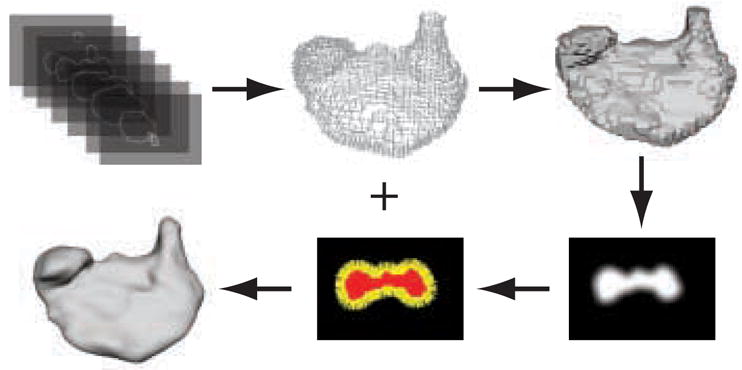
Overview of contour-based reconstruction with MPU implicit models..A point set is extracted from a stack of contours and filled to produce a binary volume. The object’s boundary is blurred and gradients are calculated at exterior voxels (boundary points) to estimate surface normals. An MPU implicit model is fit to the points and normals to produce a 3D scalar field. A mesh of the zero iso-surface is then extracted from the volume.

MPU implicit surfaces, however, also require that a surface normal be defined for every point in the point set. This information is not readily available from the input binary contours. We therefore need to estimate surface normals from the contours. Our approach for estimating normals begins by creating a 3D binary volume with explicit inside and outside information that is calculated from the closed contour data using a flood-fill algorithm. The voxels inside and on the contours are set to 1. All other voxels are set to zero. Next, a Gaussian filter is applied to the volume blurring the boundary of the 3D binary segmentation. The negative gradient of the blurred segmented volume is calculated at every original contour voxel. The calculated gradient is then used to estimate the surface normal at each contour voxel.

Given the point and normal information, MPU implicits generate a smooth 3D surface. MPU implicits use a partition of unity approach, where surface estimation is performed locally and the local implicit functions are blended together globally to produce the overall surface. They also allow for adaptive error control based on octree subdivision. See Section 3 for more details. The reconstruction quality is examined in detail through analysis and error measurements of the reconstructed models. We use an artificially created dataset with added noise in order to measure the quality of our reconstruction when the ground truth is known. Additionally, we compare our results with those produced by other methods.

2 Related Work

The problem of reconstructing 3D models from 2D contours has been studied since the 1970’s [26,38]. Numerous techniques have been proposed since that time, and fall into two main categories, contour stitching and volumetric methods. We also survey techniques for creating surfaces from sets of unorganized points.

2.1 Contour Stitching

Most of the research on contour-based surface reconstruction has focused on methods for connecting (stitching) the vertices of neighboring contours into a mesh. There are three general problems that contour stitching attempts to solve (as defined by Meyers et al. [47] and Bajaj et al. [8]):

Correspondence

Given a set of vertices in contour A and a set of vertices in contour B, a correspondence (connection) between the vertices in A must be found to the vertices in B.

Branching

Branching is a significant problem in mesh-based approaches. It occurs when one contour slice contains only one closed contour, while the next slice contains two or more closed contours. Robust techniques must be developed to determine what branches are formed between the two slices. Various methods have been proposed for this problem, while other reconstruction techniques ignore it.

Tiling

Tiling produces a mesh between two adjacent slices. The tiling process joins two slices by creating a strip of triangles using the correspondences between vertices. Most of the progress in mesh-based approaches has been made in this area.

Keppel [38] and Fuchs et al. [26] perform contour stitching between two contours P and Q by successively connecting either a vertex on P with two vertices on Q, or by connecting a vertex on Q with two vertices on P to form a triangle strip between the two contours. They use algorithms that minimize or maximize an objective function to choose the exact ordering of the vertices. Keppel’s approach attempts to maximize a function based on the volume of the polyhedron that is formed by the triangle strip. Fuchs uses a minimum path cost algorithm to find the optimal triangulation that minimizes the surface area. However, these early techniques do not deal with handling special cases such as branching. Ganapathy [28] uses a similar approach to Fuchs, but instead parameterizes each contour with a parameter t ∈ [0,1]. This parametric value is then used to guide the greedy selection of vertices on either the upper or lower contour, such that the difference between the parameter values of the current position in each contour is minimized.

Other methods that have improved on these approaches include Boissonnat [14], who uses Delaunay triangulation in the plane and then “raises” one of the contours to give the surface its 3D shape. However, this approach fails to deal effectively with some contour stitching problems such as contour pairs that are either too different from each other, or that overlap. Barequet et al. utilize a partial curve matching algorithm to connect most portions of the contours [10,11]. Then they apply a multilevel approach to triangulate the remaining portions. In later work they utilized straight skeletons to guide the inter-contour triangulation process [9]. Non-convex contour polygons also cause problems for some algorithms. Ekoule et al. [24] claim to handle dissimilar and non-convex polygons well, but use a heuristic algorithm. Meyers et al. [47] introduce a method that deals with yet more contour stitching problems. Their algorithm handles narrow valleys and branching structures using a Minimum Spanning Tree (MST) of a contour adjacency graph. Bajaj et al. [8] use various constraints on the triangulation procedure combined with contour augmentation to solve the three problems of contour triangulation (correspondence, tiling, branching) simultaneously. Fujimura and Kuo [27] use an isotropy-based method that introduces new vertices (besides those on the contours) to produce smoother meshes. They also propose to solve the branching problem by introducing an intermediate slice at the branch point between two adjacent contours. Klein et al. [40] use hardware to compute 2D distance fields. The distance fields are then used to solve the correspondence problem before surface tiling. Contours are also decimated (simplified) to a user specified level before processing. Gibson [33] creates somewhat smooth surface models from binary volume data, which we will show can be produced from stacked contours, by linking surface nodes (vertices) that are constrained within voxel regions.

Techniques for stitching together surfaces from sets of unorganized points have been studied since the early 1990’s. Edelsbrunner and Mücke [22] present a family of shapes (α-shapes) that can be defined by a point set and generated by a Delaunay triangulation-based algorithm. Bernardini et al. [13] describe an algorithm for creating surfaces from unstructured points by connecting three points that solely lie within a sphere of user-specified radius to form a triangle. The sphere is pivoted around one of the triangle’s edges until comes in contact with another point. Amenta et al. [2,3] developed a surface reconstruction algorithm based on Delaunay triangulation and 3D Voronoi diagrams. Given sufficient sampling of the underlying surface the reconstruction is guaranteed to be topologically correct. Later, Amenta et al. [5] perform surface reconstruction by first calculating a piecewiselinear approximation of the underlying surface’s medial axis transform (MAT). The surface is constructed by applying an inverse transform to the MAT. Dey et al. [4] extend this work with the Cocone algorithm, which uses complemented cones of the Voronoi diagram to provide additional guarantees about the reconstructed surface. The Cocone algorithm itself has been extended to produce water-tight surfaces [20] and to handle noisy input data [21].

2.2 Volumetric Methods

Levin [41] presents the seminal volumetric approach to surface reconstruction from a series of parallel contours. Given a distance field ² for each contour, the 2D fields are stacked and interpolated in the z-direction with cubic B-splines, producing a ℝ³ ↦ ℝ function whose zero set is the reconstructed surface. However, the reconstruction’s smoothness depends on the smoothness of the distance field, which in general only has C⁰ continuity. Raya and Udupa [55] treat the problem of time-varying, anisotropic data by interpolating intermediate contours in order to produce an isotropic sampling before performing the reconstruction. They segment greyscale volume data into contours, then convert them into 2D distance fields. These 2D distance fields are then linearly interpolated in the z-direction. Jones and Chen [37] suggest that Voronoi diagrams be used to minimize the computation needed for calculating the 2D distance fields. Barrett et al. [12] recursively apply morphological operators (dilation and erosion) to contour images in order to interpolate intermediate gray level values. This approach works well on topology maps with nested contours. Savchenko et al. [57] utilize a volume spline based on Green’s functions to create a 3D function representation of the reconstructed surface. Cohen-Or et al. [18,19] introduce the concept, without supporting results, of creating a 3D object from contours by morphing one contour into the next using warp-guided distance field interpolation. They specifically address the problem of successive contours being too far from each other (in the xy-plane). The proposed approach creates “links” between contours (features) and uses these links to guide interpolation. Chai et al. [17] present a gradient-controlled partial differential equation method for producing C¹ continuous surfaces from nested contours. Nilsson et al. [49] utilize 2D level set morphing with cross-contour velocity continuity to sweep out smooth surfaces from contour images. Whitaker [63] employs 3D level set models to partially smooth binary volumes.

2.3 Point Set Surfaces

The use of point sets as a display primitive was originally proposed by Levoy and Whitted [43]. When the screen area of the individual rendered triangles within a mesh is smaller than a pixel, it becomes more prudent to represent the model by just a set of points, e.g. its vertices. Levoy and Whitted introduced an efficient method for rendering continuous surfaces from point data.

Hoppe et al. [36] proposed one of the first implicit reconstruction methods, which produces a surface mesh from unorganized points in ℝ³ by creating a signed distance function. The distance function is estimated by the closest distance from an input point and the sign (inside/outside status) is determined by a tangent plane that locally approximates the point data. Levin [42] uses moving least squares (MLS) to approximate point sets with polynomials. Alexa et al. [1] also use point sets to represent shapes. They use the MLS approach, and introduce techniques to allow for upsampling (creating new points) or downsampling (removing points) of the surface. They also introduce a point sample rendering technique that allows for the visualization of point sets at interactive frame rates with good visual quality. Fleishman and Cohen-Or [25] extend the MLS procedure and introduce Progressive Point Set Surfaces (PPSS) to generate a base set of points that are refined to an arbitrary resolution. Xie et al. [64] further extend MLS surfaces with local implicit quadrics that allow more accurate discovery of the local topology and geometry from noisy input data. Zhao et al. [67] have employed level set models [52], represented by a distance field representation, to construct surfaces from sets of points. Amenta and Kil [6] project points onto the “extremal” surface defined by a vector field and an energy function. However, this approach requires (undirected) surface normals to be present in the point set. Another popular approach by Ohtake et al. use Radial Basis Functions [51] to define point set surfaces. In a different and much faster approach, Ohtake et al. propose the Multi-level Partition of Unity (MPU) implicit models [50]. We have chosen to build upon the MPU implicit approach in our work and describe it in detail in Section 3.

3 MPU Implicit Surfaces

Since MPU implicits approximate the input point set and have controllable error bounds, they provide a robust and effective method for reconstructing surfaces from noisy input contours. In this approach contour vertices or pixel coordinates (depending on the representation of the contours) are interpreted as points in ℝ³, i.e. a point set. The MPU function operates on the point set and reconstructs a surface that approximately fits to the input data. MPU implicit surfaces provide advantages over previous contour-based reconstruction techniques because they use local piecewise quadric functions and adapt to surface detail through the use of recursive octree subdivision. They are able to deal with unstructured points that vary in sampling density, do not require input points from a specific contour to lie on a plane, use an adaptive technique that confines the reconstruction to a specified error parameter, and are both space and time efficient.

Unlike other point set surface reconstruction algorithms [36], which utilize surface normal estimates, the MPU function requires normals to be present in the input for every data point. Ohtake et al. [50] claim that this is not a significant issue as normals can be easily obtained from a mesh representation, least-squares fitting, or obtained automatically from range acquisition devices. However, in practice this is rarely the case. Given a set of points in ℝ³ with no other information about the object on which they lie, finding surface normals for the point set is a problem on its own. Such is the case during contour reconstruction because there is no explicit structure that provides surface normals at each point. Without accurate surface normals information associated with the point set, the MPU function is unable to properly reconstruct the surface.

An MPU surface is implicitly defined by an MPU function. The MPU function defines a distance field around the surface that it represents. Globally, the MPU function is composed of overlapping local functions that are blended together, summing to one (partition of unity). A partition of unity is a set of nonnegative compactly supported functions ω_i where Σ_iω_i ≡ 1, on a bounded Euclidean domain Φ. The global function is then

$$f(x)=\underset{i}{\Sigma }{\omega }_i(x)Q_i(x),$$ (1)

where Q_i(x) is a local approximation function, see Figure 2. Each ω_i is generated by

Fig. 2.

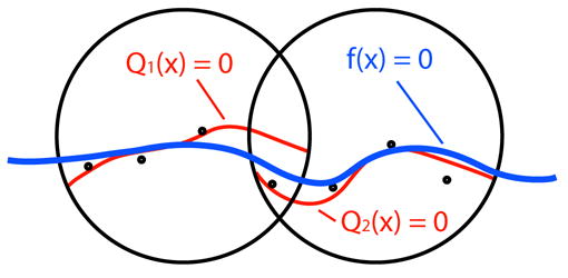
Two local approximations (red) blended to form the global function (blue).

$${\omega }_i(x)=w_i(x)/\underset{j=1}{\overset{n}{\Sigma }}{w}_j(x),$$ (2)

where the set {w_i} is a set of nonnegative compactly supported weight functions such that Φ ⊂ ∪_i supp(w_i). In the current MPU implicits implementation, each weight function w_i(x) is a quadratic B-spline. The weight functions are centered at the midpoint of each octree cell c_i in the subdivision process, and have a support radius of R_i.

MPU implicits use an adaptive octree-based subdivision scheme in order to selectively refine areas of higher detail. There are several parameters that control this subdivision process. There is a support radius R for the weight functions that is centered at the midpoint (c) of each octree cell. This support radius is initialized to R = αd, where d is the length of the diagonal of the current cell and α = 0.75· R can be enlarged if the enclosing sphere does not contain enough points, as specified by a parameter N_min. In that case, R is automatically scaled with a parameter λ: R′ = λR (λ > 1) until N_min points are enclosed by the sphere.

At each step of the algorithm, a local function Q(x) is fit to the points in the ball defined by R and centered in a cell on a leaf node of the octree. The local function’s accuracy is evaluated by calculating the Taubin distance [60], an accurate and easily-computed approximation to the shortest distance between a point and an implicit surface. It is defined by the following:

$$\epsilon =\underset{x}{max}\frac{|Q(x)|}{|\nabla Q(x)|},\forall x\in \left\{\text{ball\hspace{0.17em}defined\hspace{0.17em}by\hspace{0.17em}}R\right\}.$$ (3)

If ε is greater than a user-specified tolerance value (tol), the subdivision process continues (i.e. the current cell is divided into eight child cells and the approximation procedure is performed within each of the child cells).

The local function Q(x) is approximated in one of three ways. It can either be a 3D quadric, a bivariate quadric polynomial, or a piecewise quadric surface used for edges and corners. The function is chosen based on local surface features implied by the input normals. Our work involves biological data which by its nature does not contain sharp features. Therefore, sharp feature detection is not utilized, and as a result, only the first two quadrics are used.

The selection of one of the two functions is governed by examination of the surface normals associated with the points within the radius R. If all normals point in the same direction then a bivariate quadric is used, otherwise a general 3D quadric (which is capable of constructing two sheet functions) is used. Figure 3 explains this process in 2D: in the circle on the left, all of the normals point in the same relative direction indicating that only a bivariate quadric is needed, while in the circle on the right a two sheet general quadric is used.

Fig. 3.

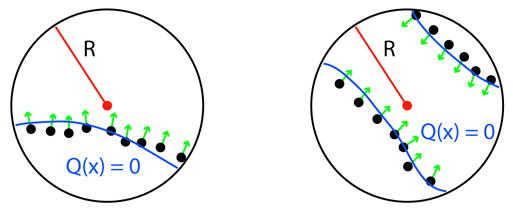
Left: bivariate quadric is used. Right: general 3D quadric is used.

4 Surface Reconstruction

Our approach to contour-based surface reconstruction interprets contour information (edge vertices or contour pixels) as a point set in ℝ³. We approximate the surface defined by the point set with MPU implicit models. In order to generate the surface, MPU implicits require not only the input points, but also normals associated with the underlying surface at each point. These normals are not provided with the raw input contours, and calculating them is the major technical issue to be addressed when applying MPU implicits to this problem domain. The generation of normals for an arbitrary set of points in space has been studied by Mitra et al. [48]. However, it is possible to exploit the structure and properties of the contour points in order to generate satisfactory, approximate normals at each point. Once normals are calculated the parameters for the MPU implicit model are adjusted to produce the desired, smooth reconstructed surface.

4.1 Surface Normal Estimation

Approximate surface normals are produced in a three step process [65]: creating a binary volume, volume filtering [59,62], and calculating the gradient of the blurred data [35] at the input points.

In our data each contour is defined by a closed set of pixels in an image. The pixels may be converted to points by using their image coordinates [i, j] as x, y coordinates and the image slice number as a z coordinate. The images themselves may be stacked to produce a 3D binary volume V_Ω has integer indices. Before stacking the images, each image is separately processed and segmented into inside and outside regions, with every pixel given an inside/outside status. Since the contours are closed a flood-fill algorithm starting at a pixel known to be outside the contours, e.g. [0, 0] may be used for the classification. Those pixels accessible from [0, 0] are labeled “outside”, and the remaining pixels are labeled “inside”. See Figure 5(a) and (b). Extra care must be taken to cope with nested contours within an image. In the resulting volume each voxel is therefore classified as lying in or on the object Ω (value 1) or outside the object (value 0). Figure 4 presents isosurfaces extracted from two binary volumes produced from stacked segmented images. The inside voxels of the resulting volume correspond directly to the points inside of each of the 2D contours.

Fig. 5.

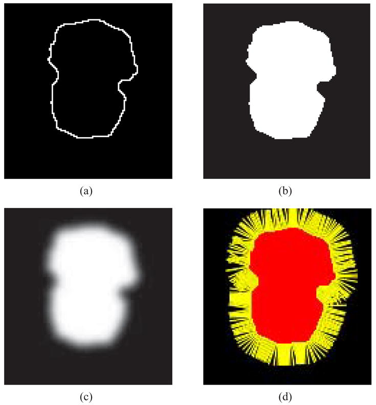
2D example of normal estimation. (a) Original contour. (b) Inside region filled. (c) After Gaussian filtering (σ = 3). (d) Normals calculated from gradient.

Fig. 4.

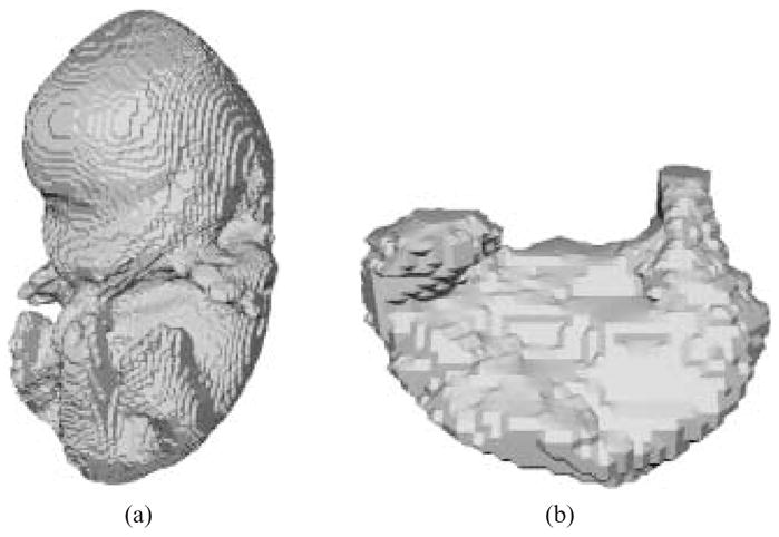
Isosurfaces extracted from binary volumes produced from stacked contours. (a) mouse embryo. (b) mouse embryo stomach.

The segmented/classified images are stacked to produce a binary volume V_Ω. A 3D Gaussian filter is applied to V_Ω in order to blur the boundary between inside and outside voxels, producing non-integer voxel values around the boundary and a smoother result. We utilize a 3×3×3 kernel defined by the 3D Gaussian function with standard deviation σ[34],

$$F(x,y,z)=\frac{1}{\sqrt{2\pi }\sigma }exp\left(-\frac{x^2+y^2+z^2}{2{\sigma }^2}\right)$$ (4)

to perform the blurring.

A 3D Sobel filter [44] is applied to the blurred volume V′ at the voxel locations associated with the original contour pixels p_l to calculate the gradient ∇V′ (p_l) at those locations. The Sobel filter was chosen because it takes into account information on the diagonals surrounding the processed point in addition to the information along the volume’s axes. However, it does place more emphasis on the axis-aligned information. The resulting gradient is normalized and negated to produce the normal associated with each input contour point,

$${\widehat{n}}_l=-\frac{\nabla V^{\prime }(p_l)}{|\nabla V^{\prime }(p_l)|}.$$ (5)

Using this approach, it is not necessary to estimate the orientation of the normals as is needed in other techniques, such as Mitra et al. [48] and Hoppe et al. [36]. Since the values of the blurred volume range from high on the inside to low on the outside of the model, the negative gradient points away from the model’s interior, which is the correct orientation for the normals. The complete process is presented in a 2D example in Figure 5.

4.2 Point and Normal Transformation

Due to the nature of some scanning processes, e.g. histologic imaging, it is possible to produce highly anisotropic data where the imaging resolution in the xy-plane is significantly greater than the slice resolution. For example, imaging resolution is only accurate to the pixel, whereas slices can be two, three, or more pixels apart from each other. Non-uniformly sampled contour data must be appropriately scaled in the z direction to ensure that points are correctly positioned in ℝ³. The transformation either increases or decreases the z component of the points to produce a consistent physical scale in all three dimensions. For example, if the in-plane xy sampling resolution is four times greater than the slicing resolution, the z component of the resulting points should be scaled by four to create points with the correct physical locations.

Since each point is simply a point in ℝ³ and not necessarily constrained to a volumetric grid, scaling each point is a straightforward procedure. However, it is first necessary to calculate surface normals from the initial binary volume before any scaling takes place. After the non-uniform scaling, the grid layout of the voxels in the volume is lost, and with it the ability to construct normals using a method based on data stored in a uniform grid. Thus the point scaling procedure must occur after the normals generation phase of the reconstruction process. Once a normal is obtained for each input point, the underlying grid structure of the points is no longer necessary and can be discarded, leaving only a list of points and their corresponding normals.

If the input points are scaled their associated normals must also be transformed. A surface normal is not a vector, but a property of the surface; normals are not invariant under anisotropic scaling. Therefore, special care must be taken to properly scale normals. For a given transformation matrix M that is applied to points on a surface, the corresponding transformation matrix A that must be applied to the normals is A = (M⁻¹)^T [61].

4.3 MPU Implicit Surface Fitting

Once the 3D point and surface normal information is obtained, the surface is reconstructed using an MPU implicit model. Two parameters control the quality and smoothness of the reconstructed MPU surface. The first is the minimum number of points (N_min) that must be included in every ball of radius R that is centered at each octree cell. The second is an error tolerance value (tol) that guarantees that the reconstructed surface lies within tol distance of the input data points. Both of these parameters are set by the user and control the quality of the reconstruction. Increasing either of the two parameters results in a higher degree of smoothing. A smaller tolerance value results in a locally tighter approximation (closer to the original data points), where the local region is defined by R. Increasing the N_min parameter while keeping tol constant results in smoother, wider regions that are still subject to the tolerance constraint. Experimentation has also shown that some values of these parameters can cause spurious surface artifacts. For example, setting the tol parameter to extremely low values can cause interpolation (as opposed to approximation) artifacts such as small spurious protrusions or dents in the surface when reconstructing noisy data. Since reconstruction and error analysis is rapidly computed, the user is able to easily and repeatedly adjust the two MPU parameters until a visually acceptable result with reasonable error statistics is produced. Currently, a heuristic approach based on experimentation is used to choose these parameter values. Future work will involve exploration of methods for automatic parameter estimation that produce the best results. MPU implicit models are also designed to deal effectively with sharp edges and corners. However, since we worked exclusively with biological data that is smooth, this feature was not deemed necessary and was disabled in our studies.

5 Reconstruction Results and Analysis

We tested and evaluated our reconstruction technique with a number of datasets. Four of the datasets (embryo, heart, stomach and tongue) are isotropic, i.e. their sampling resolutions are the same in all three dimensions. Three of the datasets (mouse brain, ventricles and pelvis) are anisotropic, with their X – Y resolution being greater than their slicing (Z) resolution. The quality of each reconstruction was quantified by calculating the distance between the input points and resulting surface. Additionally we investigated the effectiveness of MPU-based methods to reconstruct noisy input data, and compared the results from our approach to a number of other techniques and systems.

The datasets used for our studies are:

• Mouse embryo, heart, stomach, and tongue – Contours extracted from an MRI scan of a 12-day-old mouse embryo,

• Mouse brain – Contours extracted from histologic images of a mouse brain,

• Human brain ventricles – Contours extracted from a segmentation of a diffusion tensor magnetic resonance imaging (DT-MRI) scan of a human brain [68],

• Pelvis – Contours acquired from a public database at the Technion.

Table 1 presents detailed information about these datasets including number of slices, in-plane image resolution, ratio of in-plane to slice sampling rates, and total number of points (pixels) that define the contours in the dataset.

Table 1.

Characteristics of input datasets

Name	# of slices	resolution	xy:z	# of data points
embryo	186	122 ×128	1 : 1	46, 204
heart	34	89 ×98	1 : 1	4, 528
stomach	34	90 ×63	1 : 1	4, 088
tongue	32	90 ×120	1 : 1	6, 842
mouse brain	157	730 ×525	2 : 1	247, 267
ventricles	36	195 ×285	8 : 1	19, 800
pelvis	26	500 ×500	8 : 1	21, 650

All of the results from our technique presented here are displayed using flat shading, not Gouraud shading which increases the apparent smoothness of a model. Thus we present the geometry produced by our techniques as accurately as possible.

5.1 Evaluating Reconstruction Error

Although the reconstructions are visually appealing, it is necessary to quantify the quality of the reconstructions in order to determine how faithfully MPU implicit models fit to the input data. This is accomplished by calculating an error metric at the input data points that determines how well the reconstructed surface fits to the points. The metric is defined at each input point as the distance from the point to the reconstructed surface. This error calculation also provides some insight into the amount of smoothing applied by the approach to the data. Since the MPU implicit function estimates the distance to the MPU model from an arbitrary point, simply evaluating the function at each of the input data points gives the desired error value. The error values are then gathered and statistics related to the complete reconstruction are calculated. The minimum, maximum, median, arithmetic mean, and standard deviation of the error values for each reconstructed model are given in Table 2, as well as the percentage of points that are 1 and 1/2 voxel length away from the surface. All of the error metrics that are presented here are in voxel units. For example, a maximum error of 2 signifies that the contour dataset lies at most two voxels away from the reconstructed surface. The MPU parameters for these examples were determined iteratively by creating and viewing a small number of surfaces with different values, until acceptable results were produced.

Table 2.

Approximation quality of reconstructed surfaces for isotropic data with specified MPU tol and N_min parameters. Metrics are calculated in units of voxels.

name	min	max	median	mean	st dev	% < 1.0	% < 0.5	,tol	Nmin
embryo	3.0E-06	1.7273	0.2788	0.3079	0.2126	99.49	81.08	3.5	200
heart	1.5E-04	1.3217	0.2403	0.2782	0.2052	99.51	85.53	2.5	100
stomach	5.7E-05	1.4921	0.2306	0.2670	0.1994	99.73	86.33	2.5	100
tongue	6.6E-05	1.4534	0.2777	0.3151	0.2247	99.34	78.88	2.5	100
mouse brain	4.0E-06	4.2910	0.4396	0.5619	0.4794	84.14	55.30	14	350
ventricles	7.0E-06	3.6074	0.4808	0.5859	0.4652	82.01	51.62	6.5	200
pelvis	0.00	3.1170	0.2181	0.2837	0.2587	98.12	83.25	6.0	200

The reconstruction results and visualizations of the reconstruction errors are presented in Figures 6 and 7. The point sets extracted from the original datasets are first shown, followed by a color-coded reconstruction with the reconstruction error displayed from yellow (low) to red (high). The final image presents the reconstruction with areas that have errors greater than one voxel marked in red. Higher resolution final results with no error markings are presented in Figures 8 and 9. The computation times for these results (given as system time on an Apple dual 2.0 GHz G5 with 1GB of RAM) are given in Table 3.

Fig. 6.

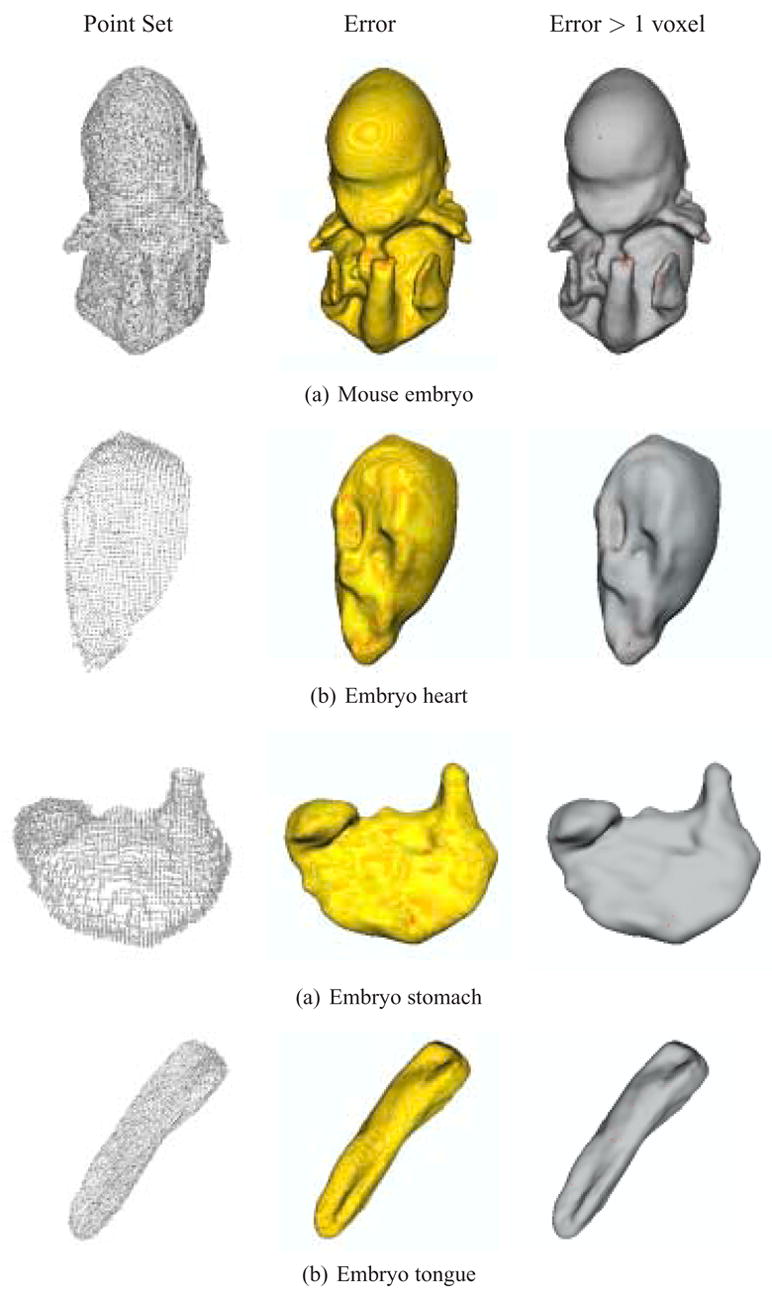
Reconstruction of isotropic mouse embryo skin, heart, stomach, and tongue data, with approximation errors. (left) Point set extracted from the input contours. (center) Reconstruction error from yellow (low) to red (high). (right) Regions with errors greater than 1 voxel marked in red.

Fig. 7.

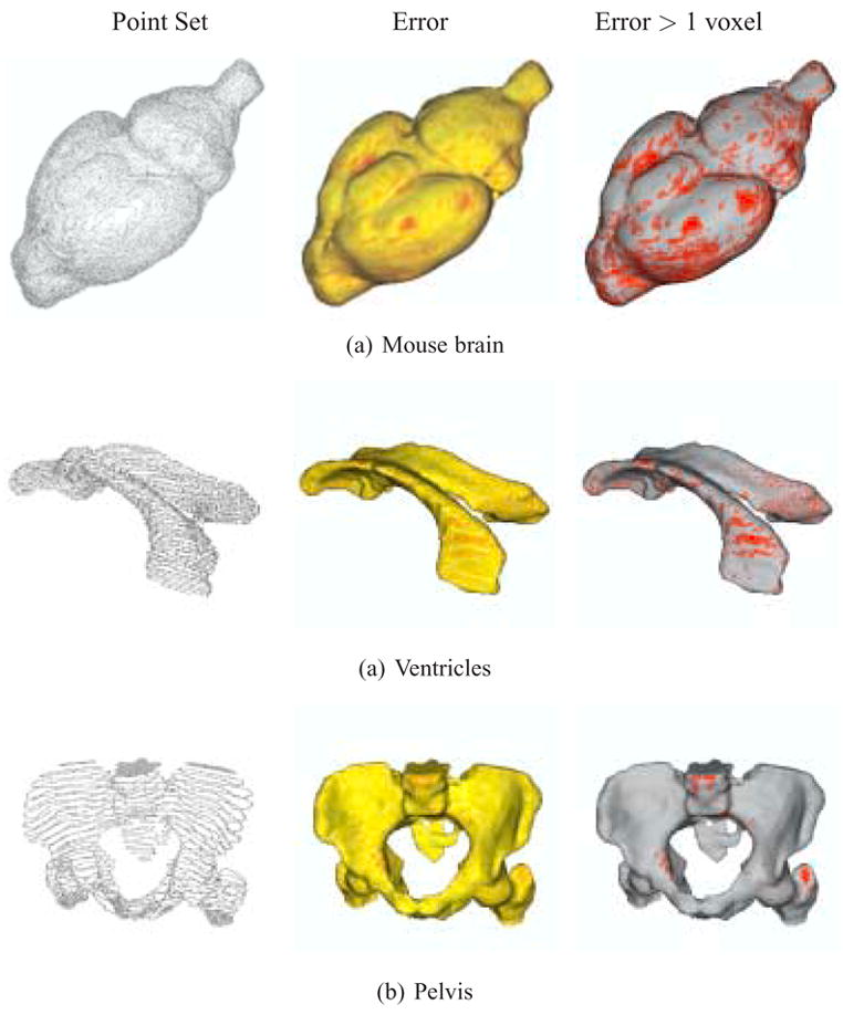
Reconstruction of anisotropic mouse brain, ventricles and pelvis data, with approximation errors. (left) Point set extracted from the input contours. (center) Reconstruction error from yellow (low) to red (high). (right) Regions with errors greater than 1 voxel marked in red.

Fig. 8.

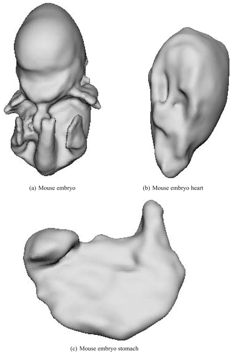
Reconstructions of the isotropic mouse embryo skin, heart and stomach datasets.

Fig. 9.

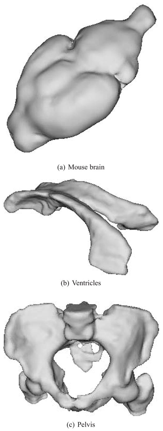
Reconstructions of the anisotropic mouse brain, ventricles and pelvis datasets.

Table 3.

Surface reconstruction execution times on an Apple dual 2.0 GHz G5 with 1GB of RAM.

name	normals estimation	surface reconstruction	total
embryo	10 sec	6 sec	16 sec
heart	1 sec	3 sec	4 sec
stomach	1 sec	5 sec	6 sec
tongue	1 sec	2 sec	3 sec
mouse brain	3 min, 14 sec	27 sec	3 min, 41 sec
ventricles	6 sec	3 sec	9 sec
pelvis	13 sec	7 sec	20 sec

While the maximum error values for the isotropic models lie between 1 and 2 voxels, the error statistics indicate that almost all regions of the reconstructed surfaces lie within the voxels defined by the original contours. For these models (embryo, heart, stomach, and tongue) most contour points are less than half a voxel-length away from the resulting MPU surface (embryo - 81.08%, heart - 85.53%, stomach - 86.33%, tongue - 78.88%). An even higher majority of points (with error measurements within three to four standard deviations) lies within one voxel of the reconstructed surface (embryo - 99.49%, heart - 99.51%, stomach - 99.73%, tongue - 99.34%). This demonstrates that the reconstruction error is sub-pixel for a vast majority of input points. The input data are provided as pixels in individual images, which are then assembled, via stacking, into voxels. The information provided to the reconstruction is discrete and represents value intervals on the order of a pixel/voxel length. Sub-pixel errors are therefore acceptable, even when an “accurate” reconstruction is desired because the surface still lies somewhere within the bounds of the original pixels, just not necessarily at their centers.

The anisotropic datasets (mouse brain, ventricles and pelvis) not only have sampling rates different from the isotropic datasets, but they also span a different range of pixel/voxel values because the in-plane resolutions of their input images are higher than the embryo datasets. In some cases, e.g. the mouse brain, the in-plane sampling resolution is nearly an order of magnitude greater than the embryo stomach dataset. Because of the difference in scales and sampling rates we have relaxed the tolerance parameter (14 for the mouse brain, 6.5 for the ventricles, and 6.0 for the pelvis datasets). This results in higher maximum values, but the means and standard deviations still stay relatively low. In fact, 84.14% of the input points for the mouse brain and 82.01% of the input points for the ventricles datasets lie within 1 voxel of their reconstructions. The pelvis dataset performs even better, with 98.12% of its input points lying within 1 voxel of the reconstructed surface. These error statistics are comparable to the small-scale, isotropic embryo dataset.

Our work has been conducted jointly with the Drexel University College of Medicine. Based on the reconstructions of the mouse brain dataset, it has been demonstrated that our approach produces accurate models and deals effectively with real-world input noise. The number of regions where the reconstruction errors are greater than one voxel are well within acceptable ranges.

Table 3 shows that the MPU-based reconstruction procedure is very fast, requiring only a few seconds to perform most surface reconstructions. The execution times for the “surface reconstruction” phase include the evaluation of the MPU function and the generation of a triangular mesh from the function. The execution time for the “normals estimation” phase includes constructing a binary volume from the contours, filtering the volume and gradient calculations. The normals calculation for the brain dataset is rather high. However, normals estimation is a one-time computation. Once points and normals have been obtained, a surface reconstruction at a desired level of quality can be achieved in only about 20 seconds. The user is able to quickly change reconstruction parameters until the desired result is obtained.

5.2 Reconstructing Noisy Contours

Several of the examples presented in this paper are produced from “real-world, noisy” datasets derived from delineations of MRI scans and histologic images, namely the heart, stomach, tongue and brain. Even though these results are visually acceptable, we also accurately measured our approach’s ability to deal with noisy input by conducting a controlled experiment on an artificial dataset. By adding a known amount of noise to an artificial dataset defined as the ground truth, we were able to accurately measure the effect of the noise and to evaluate the effectiveness of our approach on “clean” and “noisy” versions of the same dataset.

First, an artificial set of contours, defined by polylines, representing the ground truth for a specimen was created. The dataset was corrupted by adding in-plane noise as specified by [7] and [23]. The noise consists of a random in-plane shifting of a contour vertex along its normal to the contour by up to 1.4 pixels. The contour is pixelated and normals are calculated with a 2D version of the procedure described in Section 4.1. The resulting noisy contour data consists of 174 slices, each having a resolution of 204 × 231. The total number of contour points is 48,238.

Figure 10 and Table 4 present the results from our investigation. 10(a) is the original point set. 10(b) is the reconstruction produced from the uncorrupted point set with an N_min value of 100 and a tolerance value of 2. The statistics for this reconstruction in Table 4 show that 100% of the original surface (after rounding) lies within 1 voxel of the input points. The only point that lies farther away has a maximum error value of 1.041. Figure 10(c) is the reconstruction produced from the “noisy” point set with a tolerance of 2. Since it is produced with a relatively tight tolerance, the noise is evident on the model’s surface. The associated statistics are calculated with respect to the original point set and demonstrate that the reconstructed surface faithfully fits to the “clean” data. Figure 10(d) is produced by relaxing the tolerance parameter to 5. The surface is visibly smoother and the error statistics show that 83.97% of the original data are half a voxel length away and 99.80% are less than 1 voxel length from the reconstructed surface; thus providing evidence that the MPU-based reconstruction method can effectively cope with noisy contours.

Fig. 10.

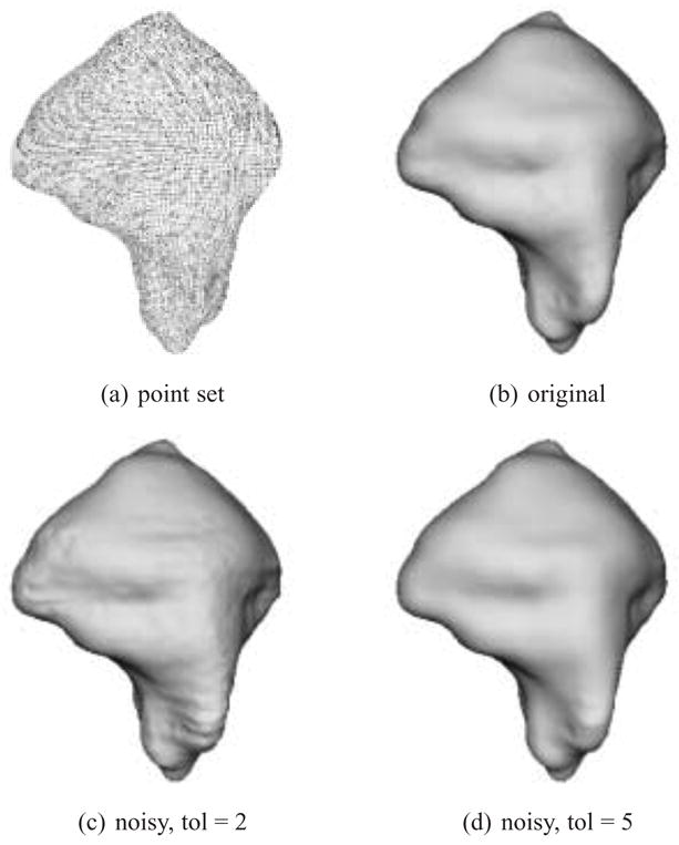
Synthetic dataset. Point set and reconstruction without noise, and reconstruction after contours are corrupted with noise.

Table 4.

Approximation quality for synthetic dataset, without and with noise. All error calculations are performed with respect to the original point set.

name	min	max	median	mean	st dev	% < 1.0 %	< 0.5	tol	Nmin
original	5.0E-06	1.0412	0.2532	0.2633	0.1672	100.00	91.00	2.0	100
noisy	7.0E-06	1.2650	0.2509	0.2723	0.1821	99.90	87.88	2.0	100
noisy	1.2E-05	1.6549	0.2695	0.2944	0.1968	99.80	83.97	5.0	100

5.3 Comparison with Other Methods

Figure 11 presents three contour-based reconstruction methods applied to similar datasets. The first result is created with a Delaunay triangulation technique provided by NUAGES [53], and is displayed with flat-shading. The middle reconstruction is produced via 2D distance field interpolation described by Klein [39,40], and is displayed with Gouraud smooth-shading. The final reconstruction is produced with the MPU implicit method, and is displayed with flat-shading. The Klein result is an image reproduced from [39], and uses a slightly different pelvis dataset from the other two results. The NUAGES and MPU implicit results are based on the same dataset. The NUAGES result demonstrates that meshing techniques produce faceted surface models and require post-processing for smoothing. The faceted nature of the Klein result is partially masked by the Gouraud-shading, but discrete artifacts can still be seen at the bottom of the model and at various locations along its silhouette. Our approach produces a naturally smooth surface without the need for any additional post-processing.

Fig. 11.

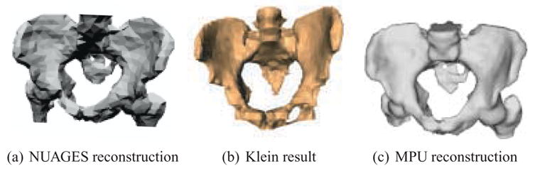
Comparing reconstruction results for similar (but not identical) pelvis datasets. (a) NUAGES reconstruction. (b) Klein [39] reconstruction (Gouraud-shaded). (c) MPU implicit reconstruction.

6 Generating Contours on Arbitrary Cutting Planes

The ability to visualize contours in arbitrary cutting planes through the reconstructed volume can aid in the analysis and understanding of a specimen. The MPU-based contour reconstruction technique, in conjunction with a fast marching method [46,58,66], produces a 3D signed distance field that may be sampled at any location. This feature easily supports the arbitrary slicing of the reconstruction. Given a user-specified plane, the field can be evaluated at regular points on the plane, producing a sampled 2D distance field. The zero contour of the 2D distance field can then be extracted and displayed.

The user defines the cutting plane with a normal, N and a value h, which is the height at which the plane crosses the centerline of the stacked contours. Given that the bounds of the reconstructed volume are (0, 0, 0) and (x_max, y_max, z_max), the centerline point z₀ is (x_max/2, y_max/2,h). We currently restrict N to point generally in the ’up’ direction; more specifically, the angle between N and the positive z-axis (ẑ) is limited to be less than 90°. The value of h is constrained to lie between 0 and z_max. The angle θ between N and ẑ is cos⁻¹ (ẑ·N). N can be mapped into the z axis by rotating θ degrees around the axis L defined by N×ẑ. Let the cutting plane have its own coordinate system u, v, n. By assuming that the origin of u, v, n is coincident with z₀ and that n is parallel with N, conservative bounds on the cutting plane can be found by mapping the reconstructed volume into the u, v, n coordinate system. This is accomplished by applying the transformation

$$\overline{\mathrm{\Gamma }}=\overline{R}(L,\theta )\overline{T}(-z_0)$$ (6)

to the set which contains the corners of the reconstructed volume, where R̄ is a transformation that rotates a point θ degrees around axis L [54], and T̄ translates a point in the given direction. is transformed into u, v, n space,

$$ℬ=\overline{\mathrm{\Gamma }}\mathcal{A},$$ (7)

to produce a set . The bounding box of (u_min, v_min, n_min), (u_max, v_max, n_max)) is then calculated. The cutting plane is regularly sampled within the rectangle defined by ((u_min, v_min,0), (u_max, v_max, 0)) and the sample points are mapped back into x, y, z space with the transformation

$$\overline{\mathrm{\Psi }}=\overline{T}(z_0)\overline{R}(L,-\theta ).$$ (8)

Evaluating the MPU function at these transformed points generates a 2D signed distance field. A zero-contour is extracted from the field to produce the final, desired result. Examples of contours generated from arbitrary cutting planes through two different reconstructions are presented in Figure 12.

Fig. 12.

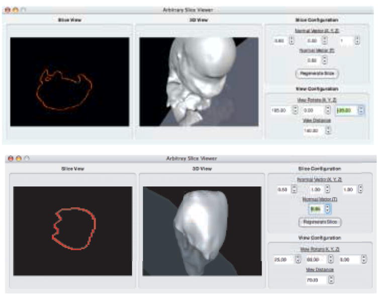
Generating contours on an arbitrary plane. Top - Through a mouse embryo reconstruction. Bottom - Through a mouse embryo heart reconstruction.

7 Conclusion

The work in this paper demonstrates that point set and implicit surface models can be applied effectively and efficiently to the problem of contour-based surface reconstruction. We have shown that it is possible to create smooth, accurate 3D surface reconstructions from contours using implicit models. In order to accomplish this, a method for surface normal estimation has been developed and applied to a number of datasets. The method uses Gaussian blurring with an edge detection algorithm in order to accurately estimate normals. Once surface normals have been estimated, Multi-level Partition of Unity (MPU) implicits are employed to reconstruct a surface from a set of input contours.

Our approach produces smooth surface models that offer sub-pixel accuracy to the original data while requiring low computation times. The reconstruction procedure has also been shown to be relatively insensitive to the sampling resolution of the original data, generating accurate reconstructions in every case. We have demonstrated that implicit surface reconstruction techniques are an effective method for processing both closely and widely spaced contours that contain noise, producing superior results in comparison with other techniques. In closing, the idea of considering a set of contours as a point set in ℝ³ creates possibilities for reconstruction of non-traditional contour data, such as non-parallel or warped contours and irregularly sampled data.

References

- 1.Alexa M, Behr J, Cohen-Or D, Fleishman S, Levin D, Silva CT. Point set surfaces; Proc IEEE Visualization; Oct, 2001. pp. 21–28. [Google Scholar]
- 2.Amenta N, Bern M. Surface reconstruction by Voronoi filtering. Discrete and Computational Geometry. 1999;22:481–504. [Google Scholar]
- 3.Amenta N, Bern M, Kamvysselis M. A new Voronoi-based surface reconstruction algorithm; Proc SIGGRAPH ’98; Jul, 1998. pp. 415–421. [Google Scholar]
- 4.Amenta N, Choi S, Dey TK, Leekha N. A simple algorithm for homeomorphic surface reconstruction. International Journal on Computational Geometry & Applications. 2002;12:125–141. [Google Scholar]
- 5.Amenta N, Choi S, Kolluri R. The power crust, unions of balls, and the medial axis transform. Computational Geometry: Theory and Applications. 2001;19(2–3):127–153. [Google Scholar]
- 6.Amenta N, Kil YJ. Defining point-set surfaces. ACM Transactions on Graphics. 2004;23(3):264–270. [Google Scholar]
- 7.Ardekani S. Inter-animal rodent brain alignment and supervised reconstruction. Master’s thesis. Drexel University; 2000. [Google Scholar]
- 8.Bajaj CL, Coyle EJ, Lin KN. Arbitrary topology shape reconstruction from planar cross sections. Graphical Models and Image Processing. 1996;58:524–543. [Google Scholar]
- 9.Barequet G, Goodrich MT, Levi-Steiner A, Steiner D. Straight-skeleton based contour interpolation. Graphical Models. 2004;66(4):245–260. [Google Scholar]
- 10.Barequet G, Shapiro D, Tal A. Multilevel sensitive reconstruction of polyhedral surfaces from parallel slices. The Visual Computer. 2000;16(2):116–133. [Google Scholar]
- 11.Barequet G, Sharir M. Piecewise-linear interpolation between polygonal slices. Computer Vision and Image Understanding. 1996;63:251–272. [Google Scholar]
- 12.Barrett W, Mortensen E, Taylor D. An image space algorithm for morphological contour interpolation; Proc Graphics Interface; 1994. pp. 16–24. [Google Scholar]
- 13.Bernardini F, Mittleman J, Rushmeier H, Silva C, Taubin G. The ballpivoting algorithm for surface reconstruction. IEEE Transactions on Visualization and Computer Graphics. 1999;5(4):349–359. [Google Scholar]
- 14.Boissonnat JD. Shape reconstruction from planar cross sections. Computer Vision, Graphics, and Image Processing. 1988;44(1):1–29. [Google Scholar]
- 15.Braude I. Master’s thesis. Drexel University; Philadelphia, PA: Aug, 2005. Smooth 3D surface reconstruction from contours of biological data with MPU implicits. [Google Scholar]
- 16.Bug W, et al. Brain spatial normalization: indexing neuroanatomical databases. In: Crasto C, editor. Neuroinformatics. Humana Press; in press. [Google Scholar]
- 17.Chai J, Miyoshi T, Nakamae E. Contour interpolation and surface reconstruction of smooth terrain models; Proc IEEE Visualization; 1998. pp. 27–33. [Google Scholar]
- 18.Cohen-Or D, Levin D. Guided multi-dimensional reconstruction from crosssections. In: Fontanella F, Jetter K, Laurent P-J, editors. Advanced Topics in Multivariate Approximation. World Scientific Publishing Co.; 1996. pp. 1–9. [Google Scholar]
- 19.Cohen-Or D, Levin D, Solomovici A. Contour blending using warp-guided distance field interpolation; Proc IEEE Visualization; 1996. pp. 165–172. [Google Scholar]
- 20.Dey TK, Goswami S. Tight Cocone: A water-tight surface reconstructor. Journal of Computing and Information Science in Engineering. 2003;3:302–307. [Google Scholar]
- 21.Dey TK, Goswami S. Provable surface reconstruction from noisy samples. Computational Geometry Theory & Applications. 2006;35:121–141. [Google Scholar]
- 22.Edelsbrunner H, Mücke EP. Three-dimensional alpha shapes. ACM Transactions on Graphics. 1994;13(1):43–72. [Google Scholar]
- 23.Eilbert J, Gallistel C, McEachron D. The variation in user drawn outlines on digital images: Effects on quantitative autoradiography. Computerized Medical Imaging and Graphics. 1990;14:331–339. doi: 10.1016/0895-6111(90)90107-m. [DOI] [PubMed] [Google Scholar]
- 24.Ekoule AB, Peyrin FC, Odet CL. A triangulation algorithm from arbitrary shaped multiple planar contours. ACM Transactions on Graphics. 1991;10(2):182–199. [Google Scholar]
- 25.Fleishman S, Alexa M, Cohen-Or D, Silva CT. Progressive point set surfaces. ACM Transactions on Graphics. 2003;22(4):997–1011. [Google Scholar]
- 26.Fuchs H, Kedem ZM, Uselton SP. Optimal surface reconstruction from planar contours. Communications of the ACM. 1977;20(10):693–702. [Google Scholar]
- 27.Fujimura K, Kuo E. Shape reconstruction from contours using isotopic deformation. Graphical Models and Image Processing. 1999;61(3):127–147. [Google Scholar]
- 28.Ganapathy S, Dennehy TG. A new general triangulation method for planar contours; Proc SIGGRAPH ’78; 1978. pp. 69–75. [Google Scholar]
- 29.Gefen S, Bertrand L, Kiryati N, Nissanov J. Localization of sections within the brain via 2D to 3D image registration; IEEE Proceedings on Acoustics, Speech, and Signal Processing; 2005. pp. 733–736. [Google Scholar]
- 30.Gefen S, Kiryati N, Bertrand L, Nissanov J. Planar-to-curved-surface image registration; Proc Mathematical Methods in Biomedical Image Analysis; 2006. in press. [Google Scholar]
- 31.Gefen S, Tretiak O, Bertrand L, Rosen G, Nissanov J. Surface alignment of an elastic body using a multi-resolution wavelet representation. IEEE Transactions on Biomedical Engineering. 2004;51:1230–1241. doi: 10.1109/TBME.2004.827258. [DOI] [PubMed] [Google Scholar]
- 32.Gefen S, Tretiak O, Nissanov J. Elastic 3-D alignment of rat brain histological images. IEEE Transactions on Medical Imaging. 2003;22(11):1480–1489. doi: 10.1109/TMI.2003.819280. [DOI] [PubMed] [Google Scholar]
- 33.Gibson S. Constrained Elastic Surface Nets: Generating smooth surfaces from binary segmented data; Proc Medical Image Computing and Computer-Assisted Intervention (MICCAI ’98); 1998. pp. 888–898. [Google Scholar]
- 34.Gonzalez R, Woods R. Digital Image Processing. 2. Prentice Hall; Upper Saddle River, NJ: 2002. [Google Scholar]
- 35.Hoehne KH, Bernstein R. Shading 3D images from CT using gray-level gradient. IEEE Transactions on Medical Imaging. 1986;MI-4(1):45–47. doi: 10.1109/TMI.1986.4307738. [DOI] [PubMed] [Google Scholar]
- 36.Hoppe H, DeRose T, Duchamp T, McDonald J, Stuetzle W. Surface reconstruction from unorganized points (Proc SIGGRAPH); Computer Graphics; 1992. pp. 71–78. [Google Scholar]
- 37.Jones M, Chen M. A new approach to the construction of surfaces from contour data. Computer Graphics Forum. 1994;13(3):75–84. [Google Scholar]
- 38.Keppel E. Approximating complex surface by triangulation of contour lines. IBM Journal of Research and Development. 1975;19:2–11. [Google Scholar]
- 39.Klein R, Schilling AG. Fast distance field interpolation for reconstruction of surfaces from contours; Eurographics ’99 Short Papers Proceedings; 1999. [Google Scholar]
- 40.Klein R, Schilling AG, Strasser W. Reconstruction and simplification of surfaces from contours. Graphical Models. 2000;62(6):429–443. [Google Scholar]
- 41.Levin D. Multidimensional reconstruction by set-valued approximation. IMA Journal of Numerical Analysis. 1986;6:173–184. [Google Scholar]
- 42.Levin D. The approximation power of moving least-squares. Mathematics of Computation. 1998;67(224):1517–1531. [Google Scholar]
- 43.Levoy M, Whitted T. Technical Report 85–022. University of North Carolina; Chapel Hill: 1985. The use of points as a display primitive. [Google Scholar]
- 44.Lyvers EP, Mitchell OR. Precision edge contrast and orientation estimation. IEEE Transactions on Pattern Analysis and Machine Intelligence. 1988;10(6):927–937. [Google Scholar]
- 45.Marker J, Braude I, Museth K, Breen D. Contour-based surface reconstruction using implicit curve fitting, and distance field filtering and interpolation; Proc International Workshop on Volume Graphics; 2006. pp. 95–102. [Google Scholar]
- 46.Mauch S. PhD thesis. California Institute of Technology; Pasadena, California: 2003. Efficient Algorithms for Solving Static Hamilton-Jacobi Equations. [Google Scholar]
- 47.Meyers D, Skinner S, Sloan K. Surfaces from contours. ACM Transactions on Graphics. 1992;11(3):228–258. [Google Scholar]
- 48.Mitra NJ, Nguyen A. Estimating surface normals in noisy point cloud data; Proc Symposium on Computational Geometry; 2003. pp. 322–328. [Google Scholar]
- 49.Nilsson O, Breen DE, Museth K. Surface reconstruction via contour metamorphosis: An Eulerian approach with Lagrangian particle tracking; Proc IEEE Visualization; 2005. pp. 407–414. [Google Scholar]
- 50.Ohtake Y, Belyaev A, Alexa M, Turk G, Seidel H. Multi-level partition of unity implicits; ACM Transactions on Graphics (Proc SIGGRAPH); 2003. pp. 463–470. [Google Scholar]
- 51.Ohtake Y, Belyaev A, Seidel H-P. A multi-scale approach to 3D scattered data interpolation with compactly supported basis functions; Proc Shape Modeling International; 2003. p. 292. [Google Scholar]
- 52.Osher SJ, Fedkiw RP. Level Set Methods and Dynamic Implicit Surfaces. Springer; Berlin: 2002. [Google Scholar]
- 53.NUAGES package for 3D reconstruction from parallel cross-sectional data. http://www-sop.inria.fr/prisme/logiciel/nuages.html.en
- 54.Pique M. Rotation tools. In: Glassner A, editor. Graphics Gems I. Academic Press; San Diego, CA: 1990. pp. 465–469. [Google Scholar]
- 55.Raya SP, Udupa JK. Shape-based interpolation of multidimensional objects. IEEE Transactions on Medical Imaging. 1990;9(1):32–42. doi: 10.1109/42.52980. [DOI] [PubMed] [Google Scholar]
- 56.Rosen G, et al. Informatics center for mouse genomics: the dissection of complex traits of the nervous system. Neuroinformatics. 2003;1:359–378. doi: 10.1385/NI:1:4:327. [DOI] [PubMed] [Google Scholar]
- 57.Savchenko V, Pasko A, Okunev O, Kunii T. Function representation of solids reconstructed from scattered surface points and contours. Computer Graphics Forum. 1995;14(4):181–188. [Google Scholar]
- 58.Sethian JA. A fast marching level set method for monotonically advancing fronts; Proceedings of the National Academy of Science; 1996. pp. 1591–1595. [DOI] [PMC free article] [PubMed] [Google Scholar]
- 59.Sramek M, Kaufman A. Alias-free voxelization of geometric objects. IEEE Transactions on Visualization and Computer Graphics. 1999;3(5):251–266. [Google Scholar]
- 60.Taubin G. Estimation of planar curves, surfaces, and nonplanar space curves defined by implicit equations with applications to edge and range image segmentation. IEEE Transactions on Pattern Analysis and Machine Intelligence. 1991;13(11):1115–1138. [Google Scholar]
- 61.Turkowski K. Properties of surface-normal transformations. In: Glassner A, editor. Graphics Gems I. Academic Press; San Diego, CA: 1990. pp. 539–547. [Google Scholar]
- 62.Wang SW, Kaufman AE. Volume-sampled 3D modeling. IEEE Computer Graphics and Applications. 1994 September;14(5):26–32. [Google Scholar]
- 63.Whitaker R. Reducing aliasing artifacts in iso-surfaces of binary volumes; Proc Symposium on Volume Visualization; Oct, 2000. pp. 23–32. [Google Scholar]
- 64.Xie H, Wang J, Hua J, Qin H, Kaufman A. Piecewise C1 continuous surface reconstruction of noisy point clouds via local implicit quadric regression; Proc IEEE Visualization; Oct, 2003. pp. 91–98. [Google Scholar]
- 65.Yagel R, Cohen D, Kaufman A. Normal estimation in 3D discrete space. The Visual Computer. 1992;8(5–6):278–291. [Google Scholar]
- 66.Zhao HK. Fast sweeping method for Eikonal equations. Mathematics of Computation. 2004;74:603–627. [Google Scholar]
- 67.Zhao H-K, Osher S, Fedkiw R. Fast surface reconstruction using the level set method; Proc 1st IEEE Workshop on Variational and Level Set Methods; 2001. pp. 194–202. [Google Scholar]
- 68.Zhukov L, Museth K, Breen D, Whitaker R, Barr A. Level set modeling and segmentation of DT-MRI brain data. Journal of Electronic Imaging. 2003 January;12(1):125–133. [Google Scholar]