A Continuum Method for Determining Membrane Protein Insertion Energies and the Problem of Charged Residues

Abstract

Continuum electrostatic approaches have been extremely successful at describing the charged nature of soluble proteins and how they interact with binding partners. However, it is unclear whether continuum methods can be used to quantitatively understand the energetics of membrane protein insertion and stability. Recent translation experiments suggest that the energy required to insert charged peptides into membranes is much smaller than predicted by present continuum theories. Atomistic simulations have pointed to bilayer inhomogeneity and membrane deformation around buried charged groups as two critical features that are neglected in simpler models. Here, we develop a fully continuum method that circumvents both of these shortcomings by using elasticity theory to determine the shape of the deformed membrane and then subsequently uses this shape to carry out continuum electrostatics calculations. Our method does an excellent job of quantitatively matching results from detailed molecular dynamics simulations at a tiny fraction of the computational cost. We expect that this method will be ideal for studying large membrane protein complexes.

INTRODUCTION

The central role of the cell membrane is to act as a selective barrier separating the cell from its environment (Lipowsky and Sackmann, 1995). The architecture of the lipid bilayer is such that hydrophobic alkyl chains are sandwiched between lipid head groups (Tanford, 1991). This arrangement shields the membrane's hydrophobic core from exposure to water and other polar or charged species in the surrounding environment (Tanford, 1991; Lipowsky and Sackmann, 1995). In addition to lipid molecules, the cell membrane is host to membrane proteins that must be embedded within the bilayer without disrupting its structural integrity. The hydrophobic nature of transmembrane (TM) segments allows membrane proteins to be maintained within the lipid bilayer without compromising cellular homeostasis (Engelman et al., 1986).

Membrane proteins account for a third of all proteins in a cell and are involved in numerous important biological functions, such as ion conduction, cell receptor signaling, and nutrient transport (Lipowsky and Sackmann, 1995; von Heijne, 2007). Although predominantly hydrophobic in nature, many TM segments contain polar and charged residues. Notably, voltage-gated K⁺ channels, cystic fibrosis transmembrane conductance regulator, and the glycine receptor, GLRA1, are all known to contain charged residues within their TM domains (Jan and Jan, 1990; Hessa et al., 2005b; Bakker et al., 2006; Linsdell, 2006). A central question in the study of membrane proteins is how charged residues can be stably accommodated within the lipid bilayer. The success of continuum electrostatics at describing the basic biophysical properties of soluble proteins leads us to ask if these approaches can also be used to understand the energetics of membrane proteins.

Biochemical partitioning experiments performed on amino acids in two-phase bulk solutions have produced amino acid hydrophobicity scales that predict a high energetic barrier for inserting charged residues into low-dielectric environments similar to the hydrocarbon core of the membrane. For instance, solvation energies for the positively charged residue arginine range from 44 to 60 kcal/mol (Wilce et al., 1995), and continuum electrostatics calculations match these values well (Sitkoff et al., 1996). In the late 60s Adrian Parsegian used continuum methods to arrive at similarly large energy barriers when considering the movement of charged ions across the membrane (Parsegian, 1969). However, a recent study introduced a biological hydrophobicity scale that challenges the long-held notion that charged residues are not easily accommodated in the low-dielectric core of the bilayer. Hessa et al. (2005a) measured the ability of the Sec61 translocon to insert a wide range of designed polypeptide sequences (H-segments) into the membrane of rough microsomes. Surprisingly, these experiments revealed that there is a very low apparent free energy for inserting charged residues into the membrane. By these methods, the apparent free energy for arginine was determined to be ∼2.5 kcal/mol.

More recently, Dorairaj and Allen (2007) performed detailed molecular dynamics (MD) simulations of a poly-leucine TM α-helix harboring a single charged arginine to probe the energetics of charged residues in lipid bilayers. They calculated the free energy profile for translating the charged residue from the upper leaflet to the lower leaflet revealing that an insertion energy of 17.8 kcal/mol is required to move the arginine to the center of the bilayer. This energy is remarkably lower than estimates based on the partitioning of side-chain analogues between bulk phases, and it makes impressive strides in understanding the translocon-derived biological energy scale. In accord with observations from the Tobias and Tieleman laboratories, one reason that this energy is much lower than previously thought is that the membrane undergoes significant bending to allow water access to the charged residue as it enters the hydrophobic core of the membrane (Freites et al., 2005; MacCallum et al., 2007). This distortion also permits the polar and charged lipid head groups to remain in favorable contact with the charged residue. However, these favorable interactions occur at the expense of introducing strain into the lipid bilayer.

The physical insight gained from careful MD simulations is indispensable, and the energetic analysis serves as a benchmark for other simulation methods. However, calculations performed with MD are computationally expensive, and we wanted to determine if much faster continuum methods could be used to quantitatively reproduce the energetics of membrane protein insertion. In the 1990s, Honig's laboratory developed the PARSE parameter set of partial charges and van der Waals radii specifically to reproduce the energetics of partitioning small molecules and analogue side chains between bulk phases (Sitkoff et al., 1994). While considering only the electrostatic and nonpolar components of the free energy of transfer, this model reproduces the experimentally determined energies quite well (Wolfenden et al., 1981). Unfortunately, applying this technique directly to membrane proteins is not straightforward. The small size and fast diffusional motion of most solvent molecules facilitate the continuum approximation of replacing the atomic details of the solution by a single dielectric value. This approximation cannot be made for lipid membranes due to their inhomogeneity. The head group region is characterized by a zone of high-dielectric value, the hydrocarbon core by a low-dielectric value, and as discussed above, the shape of the membrane–water interface can be far from planar. The largest difficulty in applying continuum electrostatics toward understanding membrane proteins is describing the geometry of the lipid bilayer around the protein. Here we use elasticity theory to determine the shape and strain energy associated with bilayer deformations. Elasticity theory has been employed to understand the geometry of membrane systems (Helfrich, 1973), and at smaller length scales it has successfully described membrane protein–bilayer interactions (Nielsen et al., 1998; Harroun et al., 1999; Grabe et al., 2003). Importantly, once the membrane shape has been determined, we feed this shape into an electrostatics calculation to determine the solvation energy of the TM helix. We show that by marrying these two theories, we are able to quantitatively match recent MD simulations at a fraction of the computational cost, demonstrating that continuum methods can be used to understand the energetics of charged membrane proteins.

MATERIALS AND METHODS

Determination of Amino Acid Insertion Energies

We designed similar peptides to those used in Hessa et al. (2005a) and calculated their electrostatic, membrane dipole, membrane deformation, and nonpolar energies in solution and in the membrane as described below. The difference between these terms computed in solution and in the membrane is the total helix insertion energy (see Fig. 1). The single amino acid energy scales shown in Figs. 2 and Figs.7 were obtained by comparing the insertion energies of two similar segments harboring different central amino acids. The energy difference between the helices is attributed to the energy difference between the central residues. Exact details for producing the amino acid energy scales are given in the online supplemental material (available at http://www.jgp.org/cgi/content/full/jgp.200809959/DC1).

Figure 1.

Cartoon diagram depicting the states used to calculate amino acid insertion energies. (A) The total energy of a reference peptide harboring between zero and seven TM leucine residues in a background of TM alanine residues is calculated in solution (left) and then in the presence of the membrane (right). In both states, the three terms in Eq. 1 or four terms in Eq. 3 are calculated. Helices were constructed using MOLDA (Yoshida and Matsuura, 1997). (B) The central residue (green) was systematically replaced by all other residues, except proline, and the energy calculations between solution and membrane were repeated. Carefully subtracting energy values computed from B with those from the reference peptide in A removes contributions to the insertion energy from the background residues as discussed in the online supplemental material.

Figure 2.

Computed biological hydrophobicity scale using a classical view of the membrane. (A) A model peptide with an arginine at the central position (green) is shown spanning a low-dielectric region representing the membrane. Helical segments with this geometry were used to produce the bar graph in B. (B) Insertion energies for 19 of the 20 naturally occurring amino acids. Amino acids are ordered according to the translocon scale (Hessa et al., 2005a). All molecular drawings were rendered using VMD (Humphrey et al., 1996).

Figure 7.

The influence of membrane bending on computing the biological hydrophobicity scale and the interplay of electrostatics and nonpolar forces. (A) Amino acid insertion energies for 17 residues calculated using our membrane-bending model (green bars) and compared with the translocon scale (Hessa et al., 2005a) (red bars) and a scale developed from MD simulations of lone amino acids (MacCallum et al., 2007) (blue bars). All three scales were shifted by a constant factor to set the insertion energy of alanine to zero (1.97 kcal/mol green, −0.11 kcal/mol red, 2.02 kcal/mol blue). The insertion energy of charged residues is reduced by 25–30 kcal/mol by permitting membrane bending. Calculations similar to those in Fig. 6 B indicate that only charged residues result in distorted membranes. (B) The energy difference between very polar amino acids and charged amino acids is quite small; however, our model predicts that the physical scenarios are quite different. The insertion penalty for asparagine is primarily electrostatic, while the nonpolar component stabilizes the amino acid (left bars). Conversely, there is very little electrostatic penalty for inserting arginine and most of the cost is associated with the nonpolar energy required to expose the TM domain to water (right bars). For comparison, we show that the classical flat membrane gives rise to a huge electrostatic penalty and a significant 6 kcal/mol membrane dipole potential penalty for arginine (middle bars).

Electrostatic Calculations

All calculations were performed using the program APBS 0.5.1 (Baker et al., 2001). Three levels of focusing were employed starting with an initial system size of 300 Å on each side. The spatial discretization at the finest level was 0.3 å per grid point. We included symmetric counter-ion concentrations of 100 mM in all calculations. In the presence of the membrane, APBS was first used to generate a set of dielectric, ion-concentration, and charge maps describing the system in solution. We developed code to then edit these 3D maps to add the effect of the membrane with the geometry determined from the solution of a separate elastostatics calculation. Once edited, the maps were read back into APBS to finish the electrostatic calculations. Dipole charges used to create the membrane dipole potential were added at the two adjacent grid points closest to the membrane core-lipid head group interface. These charges were added in plus/minus pairs so that the net charge of the system was not affected, and the value of each charge was scaled to reproduce the desired internal potential of +300 mV. Our calculations only include the influence of the membrane dipole potential on the membrane protein charges; we do not consider the secondary effect of bending a sheet of dipole charges or the reversible work associated with moving charges apart for inserting the membrane protein. For more details on editing these maps please see Grabe et al. (2004) and the online supplemental material.

Elastostatic Calculations

The shape and strain energy of the membrane was calculated using elasticity theory with typical membrane parameters taken from Nielsen et al. (1998) (Table I). In the supplemental material, we derive the finite difference scheme used to numerically solve for the membrane shape after distortion, and we discuss the solution's convergence properties. We also discuss the integration method used to determine the strain energy from the membrane shape. Finally, the height of the membrane was fed back into the electrostatic calculations to determine the dielectric environment around the inserted helix. There are many ways that this final step can be performed, but we determined that the membrane–water interface could be well fit over the entire domain by a high-order polynomial. The polynomial fit is used in the code to edit the dielectric, ion-concentration, and charge maps. The exact equation for the membrane shape is given in the online supplemental material.

TABLE I.

Parameter Values Used in All Calculations

Parameter	Symbol	Value	Reference
Water dielectric	εw	80	Floris et al., 1991
Protein dielectric	εp	2	Gallicchio et al., 2000
Membrane core dielectric	εhc	2	Long et al., 2007
Lipid head group dielectric	εhg	80	Long et al., 2007
Equilibrium membrane width	L0	42 Å	Nielsen and Andersen, 2000
Head group width	Lhg	8 Å	Lipowsky and Sackman, 1995
Ion screening concentration	Ic	100 mM	Shrake and Rupley, 1973
Bulk interfacial surface tension	α	3 × 10−13 N/Å	Jacobs and White, 1989
Area compression-expansion modulus	Ka	1.425 × 10−11 N/Å	Jacobs and White, 1989
Bending or splay-distortion modulus	Kc	2.85 × 10−10 NÅ	Jacobs and White, 1989
α/Kc	γ	1.05 × 10−3 Å−2	Jacobs and White, 1989
2 Ka/(L02·Kc)	β	5.66 × 10−5 Å−4	Jacobs and White, 1989
SASA prefactor for nonpolar energy	a	0.028 kcal/mol·Å2	Gallicchio et al., 2000
Constant term for nonpolar energy	b	−1.7 kcal/mol	Gallicchio et al., 2000

Nonpolar Energy Calculations

The solvent accessible surface area (SASA) of each transmembrane helix was calculated by treating each atom in the molecule as a solvated van der Waals' sphere (Lee and Richards, 1971). The surface of each sphere was represented by a set of 100 evenly distributed test points assigned as described in Rakhmanov et al. (1994). The fraction of test points not occluded by neighboring atoms or membrane was used to calculate the SASA of each atom, and these values were summed to give the total SASA of the protein (Shrake and Rupley, 1973). The nonpolar contribution to the solvation energy was assumed to be linearly proportional to the SASA as described in the Results.

Online Supplemental Material

The online supplemental material is available at http://www.jgp.org/cgi/content/full/jgp.200809959/DC1. We provide a detailed discussion of the calculations used to produce the computational insertion energy scales, and we show the relationship between the number of leucine residues in a TM helix and the total insertion energy in Fig. S1. Table S1 provides the energy values used to make the bar graphs in Fig. 2 B and Fig. 7 A, while Table S2 gives these values using helices optimized with the SCWRL rotamer library rather than SCCOMP. Fig. S2 shows the calculated pK_a of an arginine side chain as it penetrates the membrane, and Fig. S3 reproduces Fig. 5 D and Fig. 7 A of the main text using a head group dielectric value of 40 rather than 80.

RESULTS

Electrostatics of a Flat, Low-dielectric Barrier

Both the Honig and White groups have carefully considered the essential energetic terms relevant to inserting α helices into membranes (Jacobs and White, 1989; Ben-Tal et al., 1996). In our present study, we start with their approach. The free energy for insertion, ΔG_tot, has the following components:

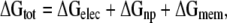(1)

where the terms on the right hand side correspond to the electrostatic, nonpolar, and membrane deformation energies, respectively. Each term is calculated with respect to the state in which the helix is in bulk aqueous solution far from the unstrained membrane.

The electrostatic contribution to helix insertion is determined by solving the Poisson-Boltzmann equation:

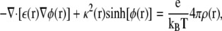(2)

where φ = eΦ/k_BT is the reduced electrostatic potential and Φ is the electrostatic potential; κ is the Debye-Huckel screening parameter, which accounts for ionic shielding; ε is the dielectric constant for each of the distinct microscopic regimes in the system; and ρ is the density of charge within the protein moiety. For a given 3D structure, we used the PARSE parameter set to assign the atomic partial charges, ρ, and the van der Waals radii to each atom. Following the PARSE protocol, we assigned ε = 2.0 to protein and ε = 80.0 to water. As can be seen in the Fig. 2 A for a flat bilayer, we started by treating the entire length of the bilayer as a low-dielectric environment with ε = 2.0. For a specific protein configuration and dielectric environment, Φ can be calculated and the total electrostatic energy determined as G_elec =∑ Φ(r_i)ρ(r_i), where the sum runs over all charges in the system.

There is a large driving force for nonpolar solutes to sequester themselves from water. This phenomenon is associated with the hydrophobic collapse of protein cores during protein folding, and it is a major consideration for membrane protein insertion into the hydrophobic bilayer. Traditionally, the hydrophobicity of an apolar solute is described in terms of the entropy loss and the enthalpy gain associated with the formation of rigid networks of water molecules around the solute. Theoretical treatments of the nonpolar energy generally assume that the transfer free energy from vacuum to water scales linearly with the SASA (Ben-Tal et al., 1996). However, detailed computational studies of small alkane molecules have shown that for cyclic alkanes the SASA is only weakly correlated with the total free energy of solvation. This is due to cyclic alkanes having a more favorable solute–solvent interaction energy, per unit surface area, as compared with linear alkanes (Gallicchio et al., 2000). Recently, it was shown that continuum methods can correctly describe these effects if they incorporate solvent accessible volume terms and dispersive solute–solvent interactions in addition to the SASA terms (Wagoner and Baker, 2006). Fortunately, helices and chain-like molecules have volumes and surface areas that are nearly proportional, and a proper parameterization of the prefactor multiplying the SASA term can effectively account for the volume dependence. Therefore, following the work of Sitkoff and coworkers, we calculated ΔG_np as the difference between the SASA of the TM helix embedded in the membrane, A_mem, and the value in solution, A_sol: ΔG_np = a·(A_mem − A_sol) + b, where the values a = 0.028 kcal/mol·Å² and b = −1.7 kcal/mol were obtained by using the equation for ΔG_np to fit the experimentally determined transfer free energies of several alkanes between water and liquid alkane phases (Sitkoff et al., 1996).

Next, we wanted to use Eq. 1 together with calculations like those shown in Fig. 2 A to address the apparent free energy of insertion for amino acids as determined by the translocon experiments (Hessa et al., 2005a). We used MOLDA to create ideal poly-alanine/leucine α helices with the central position chosen to be one of the 20 natural amino acids, excluding proline (Yoshida and Matsuura, 1997). Subsequently, we optimized the side-chain rotamer conformations with SCCOMP (Eyal et al., 2004). The free energy difference of the helical segment in solution versus the membrane, ΔG_tot, was calculated, and the insertion propensity of the central amino acid was determined by correcting for the background alanine-leucine helix (see Materials and methods). Next, we ordered the amino acid insertion energies along the x-axis according to the findings of Hessa et al. (2005a) in which the far left residue inserts the most favorably, and the insertion energetics increase monotonically going to the right (Fig. 2 B). It can be seen that the flanking residues are in qualitative agreement; our theoretical calculations show that isoleucine is one of the most favorably inserted amino acids and aspartic acid is the least favorable. Our scale is not strictly monotonic, but it does exhibit a similar trend of increasing insertion energy from left to right. The most obvious deviation from this trend occurs for the polar residues, which decrease in energy from N to Q. Also, while our calculations predict that glycine is among the least favorably inserted nonpolar residues, Hessa et al. found that glycine is clustered with the polar residues, which produces a noticeable dip in the bar graph between Y and S (Fig. 2 B).

Interestingly, the PARSE parameter set was developed to quantitatively reproduce the solubilities of side-chain analogues (Sitkoff et al., 1994), yet when we extend this work to describe the results from the translocon scale, the computational and experimental values lack quantitative agreement. Most notably the translocon scale predicts a very small apparent free energy difference between incorporating charged residues and polar residues, while our continuum electrostatic calculations predict that charged residues require 30–35 kcal/mol more energy to insert into the membrane (Fig. 2 B). While it is possible that the energetics of the translocon experiments are skewed by the close proximity of the extruded segment to the membrane, among other possibilities, part of the discrepancy surely lies in our simplified treatment of the membrane.

Elasticity Theory Determines the Membrane Shape and Strain Energy

Molecular simulations highlight two features that are missing in our continuum model. First, the membrane is not a slab of pure hydrocarbon, but rather the lipid head groups are quite polar and interact intimately with charged moieties on the protein; and second, lipids adjacent to the helix bend to allow significant water penetration into the plane of the membrane (Freites et al., 2005; Dorairaj and Allen, 2007). Both of these features can potentially reduce the energy required to insert charged residues into the membrane. Phospholipid head groups are polar and mobile, making their electrostatic nature much more like water than hydrocarbon. For dipalmitoylphosphatidylcholine (DPPC) bilayers, the width of the head group region is between 6 and 9 Å based on synchrotron studies (Helm et al., 1987), and MD simulations estimate that the corresponding dielectric value for this region is higher than bulk water (Stern and Feller, 2003). This additional level of complexity is easily accounted for by adding an 8-Å-wide intermediate dielectric region, which we assigned to ε_hg = 80, on each side of the membrane core. It is also known that membrane systems exhibit an interior electrical potential ranging from +300 to +600 mV that is thought to arise from dipole charges at the upper and lower leaflets (Jordan, 1983). While the exact nature of this potential is not known, it is thought that interfacial water, ester linkages, and head group charges may play a role. Following the work of Jordan and Coalson, we have adopted a physical model of the membrane dipole potential in which a thin layer of dipole charge is added to the upper and the lower leaflet between the head group region and hydrocarbon core (Jordan, 1983; Cardenas et al., 2000). The strength of the dipoles was adjusted so that the value of the potential was +300 mV at the center of the bilayer, far from the TM helix. While this additional energy could be considered part of ΔG_elec, we chose to call it ΔG_dipole, and we amended Eq. 1 as follows:

(3)

The much more difficult task is to determine how to model membrane defects at the continuum level. We chose to use elasticity theory, which treats the membrane surface as an elastic sheet characterized by material properties that describe its resistance to distortions such as bending (Helfrich, 1973). This method has been successfully applied to membrane mediated protein–protein interactions (Kim et al., 1998; Grabe et al., 2003) and membrane sorting based on height mismatch between the hydrophobic length of the protein and the membrane (Nielsen et al., 1998; Nielsen and Andersen, 2000). These later models are often termed “mattress models” since they allow the membrane to compress vertically much like a mattress bed does when sat upon. Simulations indicate that the membrane undergoes significant compression around buried charged groups, so we closely followed the formulation of the mattress models in our present work. The membrane deformation energy is written in terms of the compression, bending, and stretch of the membrane as follows:

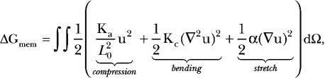(4)

where K_a is the bilayer compression modulus, K_c is the bilayer bending modulus, α is the surface tension, and u is the deviation of the leaflet height, h, from its equilibrium value, u = h − L₀/2. The total energy is given by the double integral of the deformation energy density over the plane of the membrane. A cartoon cross section of the membrane bending around an embedded TM helix illustrates the geometry in Fig. 3.

Figure 3.

System geometry corresponding to electrostatic and elasticity calculations. (A) Cross section of the deformed membrane showing the flat lower leaflet and curved upper leaflet (solid red). L₀ is the equilibrium membrane width and h is the height of the upper leaflet. The midplane is assigned z = 0 (dashed black). The radius of the TM helix is r₀ and only half of the helix is pictured. (B) The idealized helix is shown and the contact curves of the upper and lower membrane leaflets are shown in red. The lower curve is flat; however, the upper curve dips down with a minimum value at the position where the central residue resides on the full molecular helix when present.

The energy minima of Eq. 4 correspond to stable membrane configurations. The equation for these equilibrium shapes is determined via standard functional differentiation of Eq. 4 with respect to u:

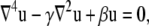(5)

where γ = α/K_c and β = 2K_a/(L₀²·K_c). We solved Eq. 5 to determine the shape of the membrane, but before doing this we had to specify the values of the membrane height and slope both far from the helix and where it meets the helix. We assumed that the membrane asymptotically approaches its unstressed equilibrium height, u = 0, far from the TM helix. Unfortunately, we do not know the height of the membrane as it contacts the helix. We started by positing the shape of the contact curve based on visual inspection of MD simulations, but later in the manuscript we will describe a systematic method for determining the true membrane–protein contact curve, which requires no a priori knowledge.

In the unstressed case, as in Fig. 2 A, we assumed that ΔG_mem is zero and that the membrane meets the helix without bending. From the MD work of Dorairaj and Allen, we observed that the upper leaflet bends to contact charged residues embedded in the outer half of the membrane (Dorairaj and Allen, 2007). The membrane appears to contact the helix at the height of the charged residue, while remaining unperturbed on the backside of the helix and along the entirety of the lower leaflet. Therefore, for the present set of calculations we only concerned ourselves with deformations in the upper leaflet, and the energy in Eq. 4 was written to reflect this assumption (see online supplemental material, available at http://www.jgp.org/cgi/content/full/jgp.200809959/DC1). We constrained the contact curve of the upper leaflet to form a sinusoidal curve against the helix with the minimum value being the height of the C_α atom of the charged residue and the maximum value being the height of the unstressed bilayer as shown in Fig. 3 B. As the depth of the charged residue changed, we adjusted the minimum value of the curve to reflect this change. We solved Eq. 5 numerically as detailed in the Materials and methods using a finite difference scheme in polar coordinates with the standard bilayer parameter values provided in Table I and taken from Huang (1986) and Nielsen et al. (1998).

The shape of the membrane when the charged residue is located at its center can be seen in Fig. 4 A. As discussed above, only the upper leaflet is deformed, and the helix is not explicitly represented at this stage, rather the membrane originates from a cylinder with a radius approximately the size of the TM segment (7.5 Å). The membrane–water interface along the radial line corresponding to the point of largest deformation is depicted in Fig. 4 B. By comparing the dashed black lines to the red line, it is clear that a significant amount of water penetration from the extracellular space accompanies this deformation, solvating residues at the helix center. However, this deformation comes at a cost; the compression and curvature introduced to the membrane results in a strain energy. The magnitude of the strain energy, ΔG_mem, is plotted in Fig. 4 C; where the far left corresponds to a compression of half the bilayer width, as shown in Fig. 4 A, and the far right corresponds to no compression at all. Importantly, the strain energy for the most drastic deformation is only ∼5.0 kcal/mol, and the energy falls off faster than linear as the upper leaflet height at the helix is increased to its equilibrium value. Localizing the penetration to one side of the membrane and one side of the helix dramatically reduces the strain energy, which is essential for this to be a viable mechanism for reducing the insertion energetics of charged residues while minimizing membrane deformation.

Figure 4.

Shape of the membrane from elasticity theory. (A) The solution to Eq. 5 was computed to determine the height of the upper leaflet of the membrane given a deformation near the origin. The membrane–water interfaces of the upper and lower leaflets are represented as two surfaces. We only show the surfaces within a 20 Å radius of the origin. The centers of the surfaces are missing since we assumed that the membrane terminates on a cylindrical helix with a radius of 7.5 Å; full molecular detail is not incorporated at this point. Calculations were performed with parameters found in Table I. (B) The membrane profile for the solution in A is shown along the axis of largest deformation. The cylinder representing the TM segment is shown at the origin (solid black lines), and the surface of the membrane is shown in red. The equilibrium height of the upper leaflet is also pictured (dashed black line) to show that a significant amount of water penetration (blue shade) accompanies membrane bending. (C) The membrane deformation energy increases as the leaflet bends with the deformation reaching a maximum of ∼5 kcal/mol.

The Electrostatics of Charge Insertion Is Minimal

Next, we used the membrane shape predicted from our elastostatic calculations to revisit the electrostatic calculations with an arginine at the central position. We assumed that the deformation of the upper leaflet does not alter the width of the high-dielectric region corresponding to the polar head groups. The helix was positioned such that the C_α atom of arginine was at the membrane–water interface (21 Å, Fig. 5 E), and then it was translated down until the C_α atom reached a height of 0 Å at the center of the membrane. For each configuration, the membrane leaflet was deformed as in Fig. 4 B so that it contacted the C_α atom, resulting in an ever-increasing membrane deformation as the arginine reached the bilayer core. The final geometry is pictured in Fig. 5 F. During peptide insertion, we calculated each term of the free energy in Eq. 3. Remarkably, the electrostatic component of the energy is essentially flat when the membrane is allowed to bend (Fig. 5 A). This result is not obvious, and it highlights the importance of the local geometry with regard to the solvation energy of charged proteins. This result will have important consequences for the mechanistic workings of membrane proteins that move charged residues in the membrane electric field as part of their normal function. Nonetheless, deforming the membrane exposes the surface of the protein to water; and therefore, it incurs a significant nonpolar energy, ΔG_np, that is proportional to the change in the exposed surface area (Fig. 5 B). Additionally, ΔG_mem increases as discussed above (Fig. 5 C). Adding together panels A–C and ΔG_dipole, we obtain the continuum approximation to the potential of mean force (PMF) for inserting an arginine-containing helix into a membrane (Fig. 5 D, solid red curve).

Figure 5.

Helix insertion energy of a model polyleucine helix with a central arginine. As the arginine enters the membrane, the upper leaflet bends to allow water penetration. At the upper leaflet, the arginine height is 21 Å, and it is 0 Å at the center. (A) The total electrostatic energy remains nearly constant upon insertion. (B) The nonpolar energy increases linearly to 18 kcal/mol as the membrane bending exposes buried TM residues to water. (C) The membrane deformation energy redrawn from Fig. 4 C. (D) The total helix insertion energy is the sum of A–C plus ΔG_dipole, which is not shown (solid red line). Correcting for the optimal membrane deformation at a given arginine depth, as shown in Fig. 6 B, produces a noticeably smaller insertion energy (dashed red line). Our continuum computational model matches well with results from fully atomistic MD simulations on the same system (diamonds taken from Dorairaj and Allen, 2007). The result from a classical continuum calculation is shown for reference (solid blue line). (E) System geometry when the arginine (green) is positioned at the upper leaflet. This configuration represents the far right position on A–D. Gray surfaces represent the lipid head group–water interface, purple surfaces represent the lipid head group–hydrocarbon core interface. The membrane is not deformed in this instance. (F) System geometry when the arginine is at the center of the membrane. This configuration represents the far left position on A–D. The shape of the upper membrane–water interface (gray) was determined by solving Eq. 5.

Continuum Calculations Match MD Simulations

Our peptide system is the one explored by Dorairaj and Allen, which allowed us to directly compare our continuum PMF with their PMF (diamonds in Fig. 5 D, adapted from Dorairaj and Allen, 2007). The shapes of both curves and their dependence on the arginine depth in the membrane are incredibly similar, despite our results (solid red line) being 3–5 kcal/mol higher than the MD simulations. Redoing the continuum calculation without allowing the membrane to bend, and neglecting the polarity of the head groups, results in the classical calculation shown in solid blue. For this model, the insertion energetics quickly rise once the charged residue penetrates the membrane–water interface, and then the energy plateaus to a value ∼15 kcal/mol larger than values predicted by the membrane-bending model or MD simulations. Allowing for membrane bending and the proper treatment of the polar head group region, brings the qualitative shape of the continuum calculations much more in-line with the MD simulations, suggesting that our calculations are capturing the correct physics of charged residue insertion into the bilayer. Additionally, we calculated the pK_a of the arginine side chain as described in the online supplemental material and found it to be close to 7 at the center of the membrane, which is in excellent agreement with the MD simulations of Li et al. (2008).

The most unsatisfying aspect of our current approach is that we have to first posit the contact curve of the membrane height against the protein. In reality, the membrane will adopt a shape that minimizes the system's total energy. A priori we have no way of knowing what that shape is, nor do we know if the shapes shown in Fig. 5 (E and F) are stable for the given arginine positions. We circumvented this shortcoming by carrying out a set of calculations in which the helix remained fixed with the arginine at the membrane center, but we varied the degree of leaflet compression. As the leaflet compresses from its equilibrium value, the electrostatic component of the helix transfer energy drops by 35 kcal/mol (see Fig. 6 A), again highlighting the importance of water penetration and lipid head group bending. Over 90% of this energy is gained by compressing the membrane down to a height of 5 Å, and very little further electrostatic stabilization is gained by compressing farther. The reason for this can be seen from Fig. 5 F in which the arginine “snorkels” up toward the extracellular space. Therefore, once the membrane height comes down to ∼5 Å, the charged guanidinium group is completely engulfed in a high-dielectric environment. When the nonpolar, lipid deformation, and membrane dipole energies are added, the energy profile produces a noticeable free energy minimum at 5 Å (Fig. 6 B). Thus, by extending our simulation protocol we have shown that these structures with deformed membranes are mechanically stable, and we have removed the uncertainty regarding the proper placement of the membrane at the protein interface.

Figure 6.

Determining the optimal membrane shape for a fixed charge in the core of the membrane. (A) Starting with the arginine at the center of the membrane as in Fig. 5 F, the helix was held fixed, and the point of contact of the upper membrane–water interface with the helix was varied from a height of 0 Å to its equilibrium width of 21 Å. The electrostatic energy decreases by 35 kcal/mol as the arginine residue gains access to the polar head groups and extracellular water. The majority of the decrease in electrostatic energy occurs from 21 to 5 Å, and there is pronounced flattening in the curve between 0 and 5 Å. (B) The total insertion energy exhibits a well-defined energy minimum at a contact membrane height of 5 Å.

Initially, we expected the curve in Fig. 6 B to exhibit a sharp jump in energy as the positively charged arginine side chain moved across the dipole charge layer interface between the membrane core and the lipid head group. However, the depth of the residue and the shape of the bending membrane smoothes out the transition and results in a 5–6 kcal/mol stabilization as the charge exits the interior of the core rather than the full 7 kcal/mol corresponding to a charge in a +300 mV potential.

Importantly, when the arginine is at the center of the membrane, the free energy is 5 kcal/mol lower if the membrane only compresses down to 5 Å rather than compressing the full half-width of the membrane (Fig. 6 B). This realization shows that the original helix insertion energy (Fig. 5 D, red curve) is wrong—it is too high. For each vertical position of the helix, we then performed a set of calculations in which we swept through all values of the leaflet thickness from 0 to 21 Å to determine the optimal compression of the membrane. These corrected energy values were used to determine the PMF of arginine helix insertion into the membrane (Fig. 5 D, red dashed curve). The results of the MD simulations and our continuum approach are now in excellent agreement, and even at the center of the bilayer the two approaches give values that differ by <1 kcal/mol. A notable difference between these methods is that we can compute the dashed red curve in Fig. 5 D in several hours on a single desktop computer, while detailed MD simulations require computer clusters and several orders of magnitude more time.

Revisiting the Calculations of Amino Acid Insertion Energies

Our initial decision to incorporate membrane bending into our computational model was motivated by the model's inability to reproduce the low apparent free energy of insertion for charged residues as determined by the translocon scale (Hessa et al., 2005a). Thus, we wanted to readdress the translocon data with our membrane-bending model. As before, we started with the helical segments inserted in the membrane with the amino acid of interest positioned at the center of the membrane as in Fig. 5 E. The upper leaflet of the membrane was then deformed until it reached the midplane of the bilayer as in Fig. 5 F, and the total insertion energy of the helix was calculated every 1 Å as the leaflet height was varied from 21 to 0. The energy minimum was identified as in Fig. 6 B and used to calculate the insertion energy of the central amino acid. The influence of the background helix was accounted for as discussed previously. Only when the central residue is charged do we observe stable minima with nonflat geometries. Therefore, our new calculations only marginally affect the energetics of the polar and hydrophobic amino acids. The model predicts that the insertion energetics of the charged residues are 7–10 kcal/mol, corresponding to a 25–30 kcal/mol reduction over the flat membrane geometry calculations. Interestingly, as observed by Hessa et al. (2005a), our model shows that a minimal amount of additional energy is required to insert charged residues compared with some polar residues. For instance, our calculations predict that inserting lysine requires only a little more than 1 kcal/mol more energy than inserting asparagine. This result is impressive, but it is important to remember that the physical scenarios are quite different for these two cases. The penalty for inserting asparagine is primarily the electrostatic cost of moving a polar residue into a flat low-dielectric environment; however, since the membrane bends in the presence of a charged residue, the penalty for arginine is not electrostatic, but rather it is the nonpolar cost of exposing the helix to water and bending the membrane (see Fig. 7 B).

While our membrane-bending model reconciles many of the observations from the translocon experiments, the magnitude and the spread of the insertion energy values are still larger for our computational scale. There are many reasons why this may be the case, and the most obvious reason is that our hypothetical situation with a single TM helix and a reference state in pure aqueous solution is an oversimplification of the full complexity of the translocon system. Thus, we wanted to compare our continuum calculations to MD simulations, which have equally well-defined states. The insertion energetics of amino acids in TM peptides have not been systematically computed via MD, so we compared our values to energies calculated for single side chains in DOPC bilayers (MacCallum et al., 2007). It is immediately evident that the insertion energetics from the continuum calculations (green bars) and the MD simulations (blue bars) have a similar spread and are well correlated with each other (Fig. 7 A). Since all three scales in Fig. 7 A represent different physical situations (a single TM helix [green], a lone side chain [blue], and a 3 TM protein [red]), we shifted each scale by a constant factor that sets the alanine insertion energy to zero. Comparing the 17 values of the corrected MD scale to the continuum scale, we see that 10 values agree to within 1.3 kcal/mol. Notably, the values for tyrosine and arginine are the largest outliers, exhibiting a difference of 5–7.5 kcal/mol between the two methods. The agreement between the continuum method developed here and the fully molecular approach is encouraging, and with the proper parameterization, it is likely that a purely continuum approach will accurately describe the energetics of membrane protein–lipid interactions. Finally, in the online supplemental text we explored the robustness of our conclusions with respect to changes in key parameters such as the dielectric value of the lipid head group region, the partial charges and atomic radii, and the choice of rotamer library; in all cases, our main conclusions are insensitive to these parameters.

DISCUSSION

We have developed a method for calculating the energetics of membrane proteins that merges two continuum theories that have on their own been very successful at describing biophysical phenomena: elasticity theory and continuum electrostatics. Electrostatic calculations with flat membranes have been considered in the past (Roux, 1997; Grabe et al., 2004), but recent experiments and simulations suggest a more dynamic role for the membrane and the charge properties of the lipid head groups (Freites et al., 2005; Hessa et al., 2005a; Ramu et al., 2006; Schmidt et al., 2006; Dorairaj and Allen, 2007; Long et al., 2007). Shape changes that correspond to deforming the membrane can be determined by solving the elasticity equation, Eq. 5. This determines the energy of bending, but it also predicts the shape of the membrane. This shape is then fed into electrostatics calculations to define the distinct dielectric regions of the membrane and the extent of water penetration around the protein. This added degree of freedom drastically reduces the electrostatic penalty for inserting charged residues into the center of the membrane at a marginal cost associated with membrane deformation.

We showed in Fig. 6 B that the contact curve of the membrane along the protein surface can be determined by considering multiple boundaries and picking the one that minimizes the free energy. Thus, the procedure is self-consistent, and it results in physically stable structures. Importantly, our continuum approach can be scaled up to treat larger protein complexes that have charged residues in or near the TM domain such as voltage-gated ion channels. However, we feel that there are several major considerations that must be addressed before extending our present methodology. First, when multiple charged residues are present on large protein complexes the contact curve will be complicated. A very efficient search algorithm must be implemented to determine the membrane shape of lowest energy. Second, for large deformations the linear approximation to membrane bending used in Eq. 5 may not be adequate; therefore, we need to consider more sophisticated models that allow for highly deformed geometries such as the finite element model of Tang et al. (2006). Third, it has been shown that the dispersion terms are needed to properly describe the nonpolar contribution to the free energy of solvation (Floris et al., 1991; Gallicchio et al., 2000; Wagoner and Baker, 2006), and the existence of fast continuum methods to do these calculations should be incorporated (see (Wagoner and Baker, 2006)). Lastly, we believe that our method will be a valuable asset to researchers considering the quantitative energetics of membrane proteins and the stability of membrane protein complexes; and furthermore, a systematic study of these systems and their interaction with the membrane as they undergo conformational changes will require fast computational methods currently not offered by molecular dynamics simulations.

References

- Baker, N.A., D. Sept, S. Joseph, M.J. Holst, and J.A. McCammon. 2001. Electrostatics of nanosystems: application to microtubules and the ribosome. Proc. Natl. Acad. Sci. USA. 98:10037–10041. [DOI] [PMC free article] [PubMed] [Google Scholar]
- Bakker, M.J., J.G. van Dijk, A.M. van den Maagdenberg, and M.A. Tijssen. 2006. Startle syndromes. Lancet Neurol. 5:513–524. [DOI] [PubMed] [Google Scholar]
- Ben-Tal, N., A. Ben-Shaul, A. Nicholls, and B. Honig. 1996. Free-energy determinants of α-helix insertion into lipid bilayers. Biophys. J. 70:1803–1812. [DOI] [PMC free article] [PubMed] [Google Scholar]
- Cardenas, A.E., R.D. Coalson, and M.G. Kurnikova. 2000. Three-dimensional Poisson-Nernst-Planck theory studies: influence of membrane electrostatics on gramicidin A channel conductance. Biophys. J. 79:80–93. [DOI] [PMC free article] [PubMed] [Google Scholar]
- Dorairaj, S., and T.W. Allen. 2007. On the thermodynamic stability of a charged arginine side chain in a transmembrane helix. Proc. Natl. Acad. Sci. USA. 104:4943–4948. [DOI] [PMC free article] [PubMed] [Google Scholar]
- Engelman, D.M., T.A. Steitz, and A. Goldman. 1986. Identifying nonpolar transbilayer helices in amino acid sequences of membrane proteins. Annu. Rev. Biophys. Biophys. Chem. 15:321–353. [DOI] [PubMed] [Google Scholar]
- Eyal, E., R. Najmanovich, B.J. McConkey, M. Edelman, and V. Sobolev. 2004. Importance of solvent accessibility and contact surfaces in modeling side-chain conformations in proteins. J. Comput. Chem. 25:712–724. [DOI] [PubMed] [Google Scholar]
- Floris, F.M., J. Tomasi, and J.L. Pascual Ahuir. 1991. Dispersion and repulsion contributions to the solvation energy: refinements to a simple computational model in the continuum approximation. J. Comput. Chem. 12:784–791. [Google Scholar]
- Freites, J.A., D.J. Tobias, G. von Heijne, and S.H. White. 2005. Interface connections of a transmembrane voltage sensor. Proc. Natl. Acad. Sci. USA. 102:15059–15064. [DOI] [PMC free article] [PubMed] [Google Scholar]
- Gallicchio, E., M.M. Kubo, and R.M. Levy. 2000. Enthalpy-entropy and cavity decomposition of alkane hydration free energies: numerical results and implications for theories of hydrophobic solvation. J. Phys. Chem. B. 104:6271–6285. [Google Scholar]
- Grabe, M., H. Lecar, Y.N. Jan, and L.Y. Jan. 2004. A quantitative assessment of models for voltage-dependent gating of ion channels. Proc. Natl. Acad. Sci. USA. 101:17640–17645. [DOI] [PMC free article] [PubMed] [Google Scholar]
- Grabe, M., J. Neu, G. Oster, and P. Nollert. 2003. Protein interactions and membrane geometry. Biophys. J. 84:854–868. [DOI] [PMC free article] [PubMed] [Google Scholar]
- Harroun, T.A., W.T. Heller, T.M. Weiss, L. Yang, and H.W. Huang. 1999. Theoretical analysis of hydrophobic matching and membrane-mediated interactions in lipid bilayers containing gramicidin. Biophys. J. 76:3176–3185. [DOI] [PMC free article] [PubMed] [Google Scholar]
- Helfrich, W. 1973. Elastic properties of lipid bilayers: theory and possible experiments. Z. Naturforsch. [C]. 28:693–703. [DOI] [PubMed] [Google Scholar]
- Helm, C., H. Mohwald, K. Kjaer, and J. Als-Nielsen. 1987. Phospholipid monolayer density distribution perpendicular to the water surface. A synchrotron X-ray reflectivity study. Europhys.Let. 4:697–703. [Google Scholar]
- Hessa, T., H. Kim, K. Bihlmaier, C. Lundin, J. Boekel, H. Andersson, I. Nilsson, S.H. White, and G. von Heijne. 2005. a. Recognition of transmembrane helices by the endoplasmic reticulum translocon. Nature. 433:377–381. [DOI] [PubMed] [Google Scholar]
- Hessa, T., S.H. White, and G. von Heijne. 2005. b. Membrane insertion of a potassium-channel voltage sensor. Science. 307:1427. [DOI] [PubMed] [Google Scholar]
- Huang, H.W. 1986. Deformation free energy of bilayer membrane and its effect on gramicidin channel lifetime. Biophys. J. 50:1061–1070. [DOI] [PMC free article] [PubMed] [Google Scholar]
- Humphrey, W., A. Dalke, and K. Schulten. 1996. VMD: visual molecular dynamics. J. Mol. Graph. 14:33–38, 27–38. [DOI] [PubMed] [Google Scholar]
- Jacobs, R.E., and S.H. White. 1989. The nature of the hydrophobic binding of small peptides at the bilayer interface: implications for the insertion of transbilayer helices. Biochemistry. 28:3421–3437. [DOI] [PubMed] [Google Scholar]
- Jan, L.Y., and Y.N. Jan. 1990. A superfamily of ion channels. Nature. 345:672. [DOI] [PubMed] [Google Scholar]
- Jordan, P.C. 1983. Electrostatic modeling of ion pores. II. Effects attributable to the membrane dipole potential. Biophys. J. 41:189–195. [DOI] [PMC free article] [PubMed] [Google Scholar]
- Kim, K.S., J. Neu, and G. Oster. 1998. Curvature-mediated interactions between membrane proteins. Biophys. J. 75:2274–2291. [DOI] [PMC free article] [PubMed] [Google Scholar]
- Lee, B., and F.M. Richards. 1971. The interpretation of protein structures: estimation of static accessibility. J. Mol. Biol. 55:379–400. [DOI] [PubMed] [Google Scholar]
- Li, L., I. Vorobyov, A.D. MacKerell Jr., and T.W. Allen. 2008. Is arginine charged in a membrane? Biophys. J. 94:L11–L13. [DOI] [PMC free article] [PubMed] [Google Scholar]
- Linsdell, P. 2006. Mechanism of chloride permeation in the cystic fibrosis transmembrane conductance regulator chloride channel. Exp. Physiol. 91:123–129. [DOI] [PubMed] [Google Scholar]
- Lipowsky, R., and E. Sackmann. 1995. Structure and Dynamics of Membranes. Elsevier Science, Amsterdam. 1052 pp.
- Long, S.B., X. Tao, E.B. Campbell, and R. MacKinnon. 2007. Atomic structure of a voltage-dependent K+ channel in a lipid membrane-like environment. Nature. 450:376–382. [DOI] [PubMed] [Google Scholar]
- MacCallum, J.L., W.F. Bennett, and D.P. Tieleman. 2007. Partitioning of amino acid side chains into lipid bilayers: results from computer simulations and comparison to experiment. J. Gen. Physiol. 129:371–377. [DOI] [PMC free article] [PubMed] [Google Scholar]
- Nielsen, C., and O.S. Andersen. 2000. Inclusion-induced bilayer deformations: effects of monolayer equilibrium curvature. Biophys. J. 79:2583–2604. [DOI] [PMC free article] [PubMed] [Google Scholar]
- Nielsen, C., M. Goulian, and O.S. Andersen. 1998. Energetics of inclusion-induced bilayer deformations. Biophys. J. 74:1966–1983. [DOI] [PMC free article] [PubMed] [Google Scholar]
- Parsegian, A. 1969. Energy of an ion crossing a low dielectric membrane: solutions to four relevant electrostatic problems. Nature. 221:844–846. [DOI] [PubMed] [Google Scholar]
- Rakhmanov, E.A., E.B. Saff, and Y.M. Zhou. 1994. Minimal discrete energy on the sphere. Math. Res. Lett. 1:647–662. [Google Scholar]
- Ramu, Y., Y. Xu, and Z. Lu. 2006. Enzymatic activation of voltage-gated potassium channels. Nature. 442:696–699. [DOI] [PubMed] [Google Scholar]
- Roux, B. 1997. Influence of the membrane potential on the free energy of an intrinsic protein. Biophys. J. 73:2980–2989. [DOI] [PMC free article] [PubMed] [Google Scholar]
- Schmidt, D., Q.X. Jiang, and R. MacKinnon. 2006. Phospholipids and the origin of cationic gating charges in voltage sensors. Nature. 444:775–779. [DOI] [PubMed] [Google Scholar]
- Shrake, A., and J.A. Rupley. 1973. Environment and exposure to solvent of protein atoms. Lysozyme and insulin. J. Mol. Biol. 79:351–371. [DOI] [PubMed] [Google Scholar]
- Sitkoff, D., K.A. Sharp, and B. Honig. 1994. Accurate calculation of hydration free-energies using macroscopic solvent models. J. Phys. Chem. 98:1978–1988. [Google Scholar]
- Sitkoff, D., N. BenTal, and B. Honig. 1996. Calculation of alkane to water solvation free energies using continuum solvent models. J. Phys. Chem. 100:2744–2752. [Google Scholar]
- Stern, H.A., and S.E. Feller. 2003. Calculation of the dielectric permittivity profile for a nonuniform system: application to a lipid bilayer simulation. J. Chem. Phys. 118:3401–3412. [Google Scholar]
- Tanford, C. 1991. The hydrophobic effect: formation of micelles and biological membranes. 2nd Edition. Krieger, Malabar, FL. 233 pp.
- Tang, Y., G. Cao, X. Chen, J. Yoo, A. Yethiraj, and Q. Cui. 2006. A finite element framework for studying the mechanical response of macromolecules: application to the gating of the mechanosensitive channel MscL. Biophys. J. 91:1248–1263. [DOI] [PMC free article] [PubMed] [Google Scholar]
- von Heijne, G. 2007. The membrane protein universe: what's out there and why bother? J. Intern. Med. 261:543–557. [DOI] [PubMed] [Google Scholar]
- Wagoner, J.A., and N.A. Baker. 2006. Assessing implicit models for nonpolar mean solvation forces: the importance of dispersion and volume terms. Proc. Natl. Acad. Sci. USA. 103:8331–8336. [DOI] [PMC free article] [PubMed] [Google Scholar]
- Wilce, M.C.J., M.I. Aguilar, and M.T.W. Hearn. 1995. Physicochemical basis of amino-acid hydrophobicity scales-evaluation of 4 new scales of amino-acid hydrophobicity coefficients derived from Rp-Hplc of peptides. Anal. Chem. 67:1210–1219. [Google Scholar]
- Wolfenden, R., L. Andersson, P.M. Cullis, and C.C. Southgate. 1981. Affinities of amino acid side chains for solvent water. Biochemistry. 20:849–855. [DOI] [PubMed] [Google Scholar]
- Yoshida, H., and H. Matsuura. 1997. MOLDA for Windows-a molecular modeling and molecular graphics program using a VRML viewer on personal computers. J. Chem. Software. 3:147–156. [Google Scholar]