Voxelwise Bayesian Lesion Deficit Analysis

Abstract

Relating cognitive deficits to the presence of lesions has been an important means of delineating structure-function associations in the human brain. We propose a voxel-based Bayesian method for lesion-deficit analysis, which identifies complex linear or nonlinear associations among brain-lesion locations, and neurological status. We validated this method using a simulated data set, and we applied this algorithm to data obtained from an acute-stroke study to identify associations among voxels with infarct or hypoperfusion, and impaired word reading. We found that a distributed region involving Brodmann areas (BA) 22, 37, 39, and 40 was implicated in word reading.

1 Introduction

Lesion-deficit analysis, in which subjects’ brain-lesion locations are related to their neurological status, plays an important role in studies aiming to identify structure-function associations in the human brain (Berker et al. (1986); Damasio et al. (1996); Tyler and Malessa (2000)). Structural magnetic-resonance (MR) examination enables neuroscientists to identify brain lesions in vivo, and thus is central to lesion-deficit analysis.

The analysis of lesion-deficit studies depends on how the clinical and image data are represented. The clinical variable, C, representing neurological status, may be either continuous, such as mean reaction time for word recognition, or discrete, such as the presence or absence of Broca’s aphasia. With regard to spatial resolution, lesion-deficit analysis methods can be classified into two general categories: voxel-based and region-of-interest (ROI) based. ROI-based methods are valuable in assessing the functional role of a specific region (Chao and Knight (1997); Friedrich et al. (1998)). Voxel-based methods treat each voxel as a spatial variable, and are thus complementary to ROI-based methods. Assuming that a ROI consists of voxels that have similar associations with the clinical variable, treating these voxels as a single ROI variable will increase statistical power relative to voxel-based methods. However, if a ROI consists of subregions that do not have similar associations with the clinical variable, grouping these subregions together could decrease statistical power.

Voxel-based lesion-deficit methods include MAP3 (Damasio et al. (1996)), voxel-based lesion-symptom mapping (Bates et al. (2003)), voxel-based χ² computation (Karnath et al. (2004)), voxel-based logistic regression (Karnath et al. (2004)), and voxel-based correlation (Tyler et al. (2005)). For each voxel, MAP3 (Damasio et al. (1996)) calculates the difference between the number of subjects having both a lesion and the deficit, and the number of subjects having a lesion but no clinical deficit. In voxel-based lesion-symptom mapping (Bates et al. (2003)), a voxelwise t-test comparing scores between subjects with and without lesions is computed. In voxel-based χ² test (Karnath et al. (2004)) computation, a 2 × 2 table is generated based on the clinical variable (deficit/no deficit) and lesion frequency (number intact/number damaged), from which a χ² statistic is computed. Voxel-based logistic regression (Karnath et al. (2004)) is based on two independent variables, overall lesion volume and whether or not a voxel was damaged for a subject; these two variables are used to predict the binary clinical variable. The resulting Z-scores constitute a statistical map. In voxel-based correlation (Tyler et al. (2005)), behavioral measures and MR signal intensity are correlated using a general linear model (GLM).

We propose a Bayesian data-mining method, voxelwise Bayesian lesion deficit analysis (vBLDA), for voxel-based lesion-deficit analysis. The differences between our proposed method and other voxel-based analysis methods are four-fold. First, our method is nonparametric: it does not rely on statistical assumptions, such as normality, that constitute the basis of voxelwise t-statistic computation and voxel-based correlation. Second, vBLDA is multivariate, whereas the other methods listed above are mass-univariate. vBLDA has the potential to detect nonlinear, multivariate associations among lesion locations and the status of a clinical variable, which would not be detected by univariate approaches. Third, vBLDA is fully automated: it requires no user input, such as ROI specification (as would be the case for ROI-based approaches) or a predefined significance threshold (as would be the case for mass-univariate voxelwise approaches). Fourth, our method explicitly models spatial correlations among voxels in MR images. Methods that do not incorporate such spatial correlations could be too conservative when thresholding statistical maps (Brett (1999)).

Our contributions are as follows. First, we propose a novel voxel-based lesion-deficit analysis method, vBLDA. The proposed method is closely related to Bayesian-network lesion-deficit analysis (BLDA) described in Herskovits and Gerring (2003). BLDA used Bayesian networks to represent lesion-deficit associations for atlas structures, and employed a greedy-search algorithm to find a locally optimal Bayesian-network model. The connection between BLDA and vBLDA is that both of them use a Bayesian-network representation to model lesion-deficit associations among brain regions and the clinical variable. The major difference between vBLDA and BLDA is that vBLDA is voxel-based, whereas BLDA is atlas-based. Generating the Bayesian-network model at the voxel level is much more complicated than doing so at the atlas level, due to the substantially increased size of the model space. Second, we evaluate vBLDA’s performance by analyzing a study designed to identify brain regions that are critical for word reading. We compare this analysis with the BLDA analysis for the same data set. In addition, we compare vBLDA to mass-univariate for the analysis of simulated data manifesting nonlinear multivariate associations among lesion locations and a clinical variable.

2 Materials

2.1 Simulated data

In this experiment, we synthesized data for a study consisting of two groups of 12 subjects, for a total of 24 subjects. Subjects in group 1 were clinically normal with respect to a binary clinical variable (C=0), whereas those in group 2 manifested a clinical deficit (C=1). For subjects in group 2, we simulated the data such that we ensured that one of two regions, the left caudate nucleus (CN) or the left supramarginal gyrus (SG), was damaged with equal probability, that no subject had damage to both regions, and that damage in either brain region causes the cognitive deficit (C=1). Let [CN=damaged, SG=intact, C=deficit] represent a simulated subject in whom the left caudate nucleus is damaged, the left supramarginal gyrus is not damaged, and the subject manifests the clinical deficit. In this simulated study, we generated 6 subjects with [CN=damaged, SG=intact, C=deficit], and another 6 subjects with [CN=intact, SG=damaged, C=deficit].

We synthesized lesion data for 24 subjects, based on diffusion weighted imaging (DWI) sequences acquired from subjects with acute ischemic stroke. DWI was acquired with b_max = 1000 s/mm² and TR/TE = 10,000 msec/120 msec. For each subject, two clinical experts manually delineated regions of acute ischemia. From these manually labeled regions of acute ischemia, we generated a binary lesion map for each subject, in which a voxel with value ‘1’ represented ischemic tissue, while a voxel with value ‘0’ manifested no evidence of restricted diffusion. We registered each subject’s diffusion images to the MNI Jakob template (Kabani et al. (1998)), using a mutual-information–maximization algorithm (Jenkinson and Smith (2001)). This registration step generated a deformation field for each subject. In applying this deformation to the lesion map, we obtained lesion maps defined in the template space. For subject i, we denote the lesion map defined in the template space by Ψ_i.

Group 1 consisted of subjects without clinical deficit. We simulated such that we ensured that subjects in this group had lesions in the right hemisphere only. We used lesion maps from the acute ischemic-stroke study as the lesion maps for the right hemisphere, omitting left-hemispheric lesions. Of note, the stroke patients had relatively few lesions in the right hemisphere.

For subject i in group 2, we used a lesion map from the acute ischemic stroke study as the lesion map for one of the two regions (CN and SG). In particular, we intersected a CN or SG mask with the lesions derived from Ψ_i; lesions outside the mask was omitted. For example, for a subject with [CN=damaged, SG=intact, C=deficit], we intersected the lesion map derived from Ψ_i with the CN mask (CN=damaged), but not with SG mask (SG=intact). We chose to focus on CN and SG because we observed that the stroke subjects had relatively large numbers of lesioned voxels in these regions, thus guaranteeing that the simulated data would have enough lesions in these regions to detect a difference from group 1.

2.2 A study of acute ischemic left-hemispheric stroke

We analyzed data collected from 33 patients with acute ischemic left-hemispheric stroke, whose ages ranged from 19 to 86 (mean 58.3 ± 15.7). Within 24 h of stroke onset, these subjects attempted a word-reading battery (Hillis et al. (2001a)). If a subject had an error rate greater than two standard deviations above the mean from previous studies of hospitalized control subjects (Hillis et al. (2002)), this subject was classified as having word-reading impairment. Overall, there were 18 subjects with impaired word reading. We denote whether a subject had impaired word reading by the clinical variable C, which assumes the value ‘0’ (no impairment) or ‘1’ (impairment).

All subjects underwent DWI and perfusion-weighted imaging (PWI) as part of the Johns Hopkins Acute Stroke Protocol, within 24 h of symptom onset. DWI was acquired with b_max = 1000 s/mm², and TR/TE = 10,000 msec/120 msec. PWI was acquired with TR/TE = 20,000 msec/60 msec, with 20 cc Gadolinium-DTPA injected intravenously at 5 cc/sec. Combining DWI and PWI, we can identify voxels with tissue dysfunction due to either hypoperfusion or acute ischemia. Two experts, blinded to the results of the reading test, manually delineated regions of acute ischemia. We identified regions of hypoperfusion automatically after spatial registration, by comparing each voxel to its contralateral counterpart, and identifying time-to-peak differences of 4 sec or greater. The inter-rater reliability for identifying abnormal (i.e., with respect to diffusion or perfusion brain regions across the two experts was very high (96% point to point agreement).

To align spatial information across and within subjects, we registered each subject’s MR images to a common stereotaxic space. In particular, we registered each subject’s DWI and PWI images to the MNI Jakob template, using a mutual-information maximization algorithm (Jenkinson and Smith (2001)), and saved the resulting spatial transformation. We then applied this transformation to the manually delineated ROIs, generating an infarct map defined in MNI coordinates. We applied the same transformation to the PWI images. Finally, for a voxel in the MNI space, if it was infarcted in the normalized DWI image or hypoperfused in the normalized PWI image, this voxel was labeled as abnormal (i.e., lesioned). In this manner, these image-preprocessing steps generated a binary lesion map for each subject. We labeled each voxel in a lesion map ‘1’ if it represented ischemic or hypoperfused (i.e., lesioned) tissue; otherwise, we labeled that voxel ‘0’ (i.e., normal).

3 Methods

3.1 Background: Bayesian networks

Our approach to voxel-wise lesion-deficit analysis is based on a Bayesian-network representation. A Bayesian network B is a probabilistic graphical model of a joint distribution (Pearl (1988)). In a Bayesian network, the joint distribution over a set $\mathcal{V}=\{X_1,X_2,\dots ,X_n\}$ is represented by a product of conditional probabilities. That is,

$$P(\mathcal{V})=\prod _{i}P(X_i|pa(X_i)),$$ (1)

where $pa(X_i)\subseteq \mathcal{V}$ is a set of variables called the parents of X_i. The graphical representation S, which is referred to as the structure of a Bayesian network, is a directed acyclic graph. $S=(\mathcal{V},\mathcal{E})$, where $\mathcal{E}$ contains all edges from pa(X_i) to X_i. Figure 1 depicts an example of a Bayesian network, which represents the associations among lesions in three brain regions (Brodmann area (BA) 22, BA 37, and BA 39), and the presence or absence of a reading deficit. The joint distribution can be represented as

Figure 1.

An example of a Bayesian network representing lesion-deficit associations

$$\begin{array}{l}P(BA22,BA37,BA39,\mathit{deficit})\\ =P(BA22)P(BA37)P(BA39|BA22,BA37)P(\mathit{deficit}|BA39).\end{array}$$ (2)

In this example, $\mathcal{E}=\{BA22\to BA39,BA37\to BA39,BA39\to \mathit{deficit}\}$ S corresponds to a series of conditional-independence statements. For example, in the Bayesian network in Figure 1, a subject’s ability to read is conditionally independent of the states of BA 22 and BA 37, given knowledge of whether there is a lesion in BA 39. That is, once we know the state of BA 39 for a particular subject, knowing the states of BA 22 or BA 37 provides no further information about the probability of that subject’s having a reading deficit.

In this manuscript, we assume that voxels are binary, assuming values in {0, 1}, where ‘0’ and ‘1’ represent no lesion and lesion, respectively. We also assume that the clinical variable is binary (no deficit or deficit, and denoted by ‘0’ and ‘1’). Since all variables are discrete, we adopt the discrete Bayesian-network representation, in which P(X_i | pa(X_i)) is represented as a conditional-probability table (CPT). As shown in Figure 1, each entry in a CPT, denoted by θ_ijk, represents P (X_i = k | pa(X_i) = j). For example, in Figure 1, P(deficit = present | BA39 = lesion) = 0.78, which means that the probability of a subject’s having a deficit is 0.78 when in the setting of lesions in BA 39. Θ = {θ_ijk} is referred to as the set of parameters, or conditional probabilities, for a Bayesian network. The pair {S, Θ} constitutes a Bayesian-network model.

When used to model associations among variables, Bayesian networks have two major strengths compared to standard statistical approaches. First, a Bayesian network can represent any multivariate probabilistic association among discrete variables (Pearl (1988)). Second, Bayesian networks inherently encode uncertainty (Pearl (1988)), rendering these models robust to noisy data.

An important issue in data modeling using Bayesian networks is to generate a Bayesian-network model from data. For this purpose, we require a metric to evaluate how well a Bayesian-network structure S models data D, while penalizing increasing model complexity to avoid over-fitting. The most widely used such metric is the K2 score (Cooper and Herskovits (1992); Herskovits (1991)). In a Bayesian network, the marginal likelihood P(D | S) can be represented as P(D | S) = ∫ P(D | Θ, S)P(Θ | S)dΘ. The K2 score, as the marginal likelihood, can be represented as

$$K2(S,\mathbf{D})=\prod _{i=1}^n\prod _{j=1}^{q_i}\frac{(r_i-1)!}{(N_{ij}+r_i-1)!}\prod _{k=1}^{r_i}{N}_{\mathit{ijk}}!,$$ (3)

where r_i and q_i are the number of possible states of X_i and pa(X_i), respectively, and N_ijk is the number of instances in which the variable X_i assumes state k and pa(X_i) assumes joint state j. As shown in (Herskovits (1991)), the K2 score can be decomposed into two components: one that favors models that best fit the data, and one that favors models that are parsimonious. Bayesian-network data-analysis algorithms typically seek to maximize the K2 score, or a similar metric. In general, due to the sheer size of the model space, which is exponential in the number of variables, one cannot perform exhaustive search for the optimal Bayesian-network structure S*; rather, heuristic search is employed to find S*.

Given a fixed structure, the maximum-likelihood estimation of parameters Θ is:

$${\widehat{\theta }}_{\mathit{ijk}}=\frac{N_{\mathit{ijk}}+1}{N_{ij}+r_i}$$ (4)

3.2 Rationale

Our overall goal in implementing lesion-deficit analysis is the identification of voxels that best characterize group differences; in other words, we seek to identify the set of voxels that is most predictive of group membership (deficit versus no deficit).

Many lesion-deficit studies (Damasio et al. (1996); Herskovits et al. (1999); Karnath et al. (2004); Tyler et al. (2005)), demonstrated that voxels critical to a particular neurological function are not randomly distributed in the brain; rather, they tend to co-locate in particular regions. However, for different brain regions, the association between the region’s status and the clinical variable could be different (Herskovits and Gerring (2003)). The Bayesian network depicted in Figure 1 provides a hypothetical example. Since the associations among lesion regions and C can be described as a joint distribution, and since discrete Bayesian networks can represent arbitrary joint distributions among discrete variables, we can use a discrete Bayesian network to represent all associations among brain regions and the clinical variable.

A crucial concept in Bayesian-network modeling is that of a Markov blanket. The Markov blanket of node X_i, denoted by mb(X_i), is the minimum set such that all other variables are rendered conditionally independent of X_i given mb(X_i). In S, mb(X_i) is identified as the union of the parents of X_i, the children of X_i, and the parents of the children of X_i. Variables in mb(X_i) are most strongly associated with X_i and jointly have the most predictive power about the state of X_i. Therefore, if we use a Bayesian network to represent the joint distribution among brain regions and a clinical variable, the regions critical to predicting the clinical variable constitute the clinical variable’s Markov blanket.

To identify regions in mb(C) based on observed data, we must (1) group voxels into regions, and (2) use a Bayesian-network generation algorithm to generate a network structure S, and identify mb(C) based on S. We call task 1 voxel-space partitioning, and we call task 2 Markov-blanket identification. The choice of the partitioning method is critical to the success of this approach, as the results of partitioning directly affect Markov-blanket identification. For example, assume that a region, consisting portions of BA 22 and BA 37, is critical to C. If we use a Brodmann atlas to partition the voxel space, we would split this region into two parts, in which case Markov-blanket identification might not identify either BA 22 or BA 37, because splitting the region region into two parts decreases statistical power. However, combining these two steps, i.e., directly searching the space of possible partitions and the most plausible model corresponding to each partition, is infeasible due to the very high dimensionality of the partition and model spaces.

In our approach, we iteratively perform voxel-space partitioning and Markov-blanket identification. The output of the proposed method is a model M = {B, Λ}, where Λ represents identified regions characterizing C, and B is a Bayesian network that quantifies the associations among regions and C. To reduce computational complexity, we utilize a specific type of Bayesian network, depicted in Figure 2: a Bayesian network with inverse-tree structure, in which C is a leaf node, and all other variables are parents of C. Restricting the space of possible Bayesian-network models to those with inverse-tree structure greatly reduces the size of the candidate-model space. We have proved that mb(C) as identified by this approach is a subset of the Markov blanket of C in the underlying Bayesian network (Chen and Herskovits (2005a)). That is, if the true Bayesian network representing associations among the regions and C is B*, our approach will not add regions to mb(C) that are not in mb(C) in B*.

Figure 2.

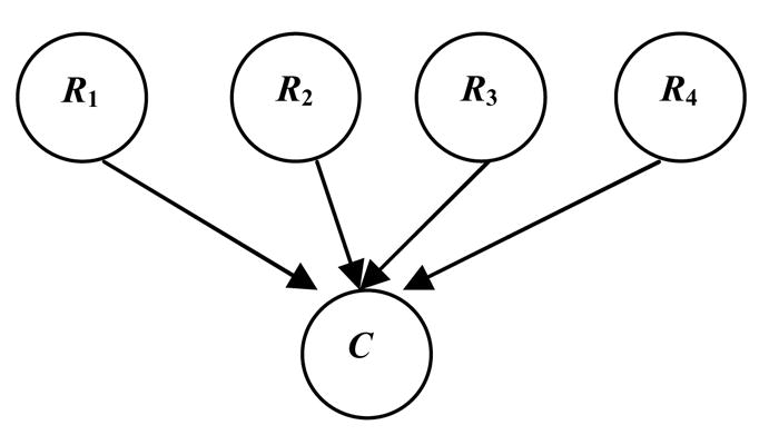
A Bayesian network with inverse-tree structure

3.3 Algorithm

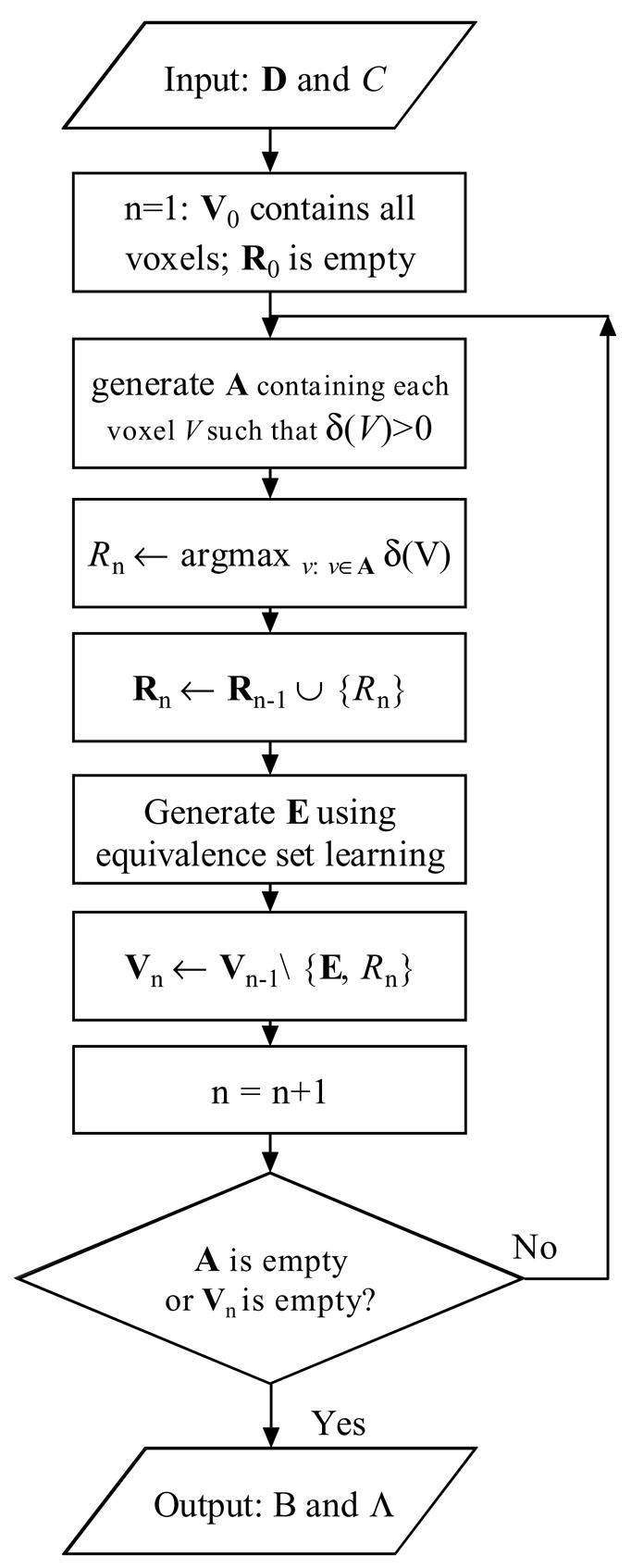
An overview of our voxel-wise Bayesian lesion-deficit-analysis algorithm is shown in Figure 3. The input is a data set D for m subjects, consisting of C and subjects’ lesion maps. The output is a model M = {B, Λ}, characterizing the associations among voxel groups and C.

Figure 3.

Voxelwise Bayesian lesion-deficit analysis

Our algorithm iteratively performs Bayesian-network generation (Markov blanket identification) and equivalence-set generation (voxel-space partitioning). Details of Bayesian-network generation and equivalence-set generation are described in Chen and Herskovits (2005b).

Bayesian-network generation identifies a set of representative voxels R* ={R₁, R₂, …, R_k}such that

$${\mathbf{R}}^{\ast }=\underset{\mathbf{R}:pa(C)=\mathbf{R}}{argmax}K2(S,\mathbf{D}),$$ (5)

where pa(C) = R in S. These representative voxels are jointly highly informative about C. Exhaustive search of R* is infeasible due to the high dimensionality of the model space. Therefore, we employ greedy search to find R*. For step n, let R_n and V_n denote the representative voxel set, and the candidate voxel set in which we search for the representative voxel, respectively. We begin with a model including R₀ = Ø, and V₀ including all voxels. In step n, for voxels in V_n−1, we search for R_n such that

$$R_n=\underset{V:\delta (V)>0}{argmax}\delta (V),$$ (6)

where δ(V) is defined as K2(S^new, D) − K2(S^old, D)), pa(C) = {V} ∪ R_n−1 in S^new, and pa(C) = R_n−1 in S^old. We add R_n to the representative-voxel set. Then we find all voxels that are probabilistically equivalent to R_n. We denote this set of voxels by E; we describe this step in the next paragraph. Then we generate V_n as V_n−1\{E, R_n}. Bayesian-network generation continues to add variables until none of remaining variables can increase the K2 score when added to the model or V_n is empty.

For representative voxel R_i, equivalence-set generation detects voxels that are probabilistically equivalent to R_i. In stating that a voxel V is probabilistically equivalent to voxel R_i, we mean that the conditional-probability distribution P(V | C) is similar to the distribution P(R_i | C). Equivalence-set generation is based on a similarity metric, which measures probabilistic equivalence between V and R_i. We use the metric s(V, R_i) = P (V = 1, R_i = 1) + P(V = 0, R_i = 0) to define probabilistic equivalence between binary variables V and R_i. This similarity metric does not explicitly encode information about C. Instead, for each R_i, we search a subset of voxels A, rather than the entire voxel set, to generate the equivalence set. A contains all voxels V′ such that δ(V′) > 0, because R_i satisfies the condition δ(R_i) > 0.

For each R_i, we obtain a similarity map S for voxels in A. Based on S, we use a clustering algorithm to group voxels A into clusters. We label those voxels that are in the cluster with the highest mean similarity metric as being probabilistically equivalent to R_i. The clustering algorithm we use is the belief-map generation algorithm described in (Chen and Herskovits (2005b)). This algorithm is accurate and computationally efficient, and automatically determines the optimal number of clusters.

To incorporate spatial information, we utilize Markov random fields to model spatial correlations during equivalence-set generation; this feature increases the tendency for our algorithm to include spatially contiguous voxels in the same cluster. In this step, each voxel V_i in A is associated with an unobserved label L_i, which represents the cluster to which this voxel belongs. We use a pairwise Markov random field as the spatial model for these labels. Let μ_a be the mean similarity metric for cluster a. In this Markov random field, for two nearby voxels V_i and V_j, if L_i and L_j are in clusters a and b, and μ_a and μ_b are approximately equal, the probability of observing this pattern will be greater than the probability of observing the pattern in which μ_a and μ_b differ greatly. In this manner, the Markov random field implements spatial smoothness.

The final output of vBLDA is a model M = {B, Λ}, where B is a Bayesian network with inverse-tree structure, and Λ represents regions that best predict C, within the limits of our search algorithm. Figure 4 depicts vBLDA schematically, including Bayesian-network generation and equivalence-set generation.

Figure 4.

An overview of the vBLDA algorithm.

In the Bayesian network generated by vBLDA, variables are either voxels in the representative-voxel set or C; the parent set of C is the representative-voxel set R*. We use equation (4) to estimate the parameters of B. Λ is defined in the stereotaxic space; each representative voxel R_a in R* is associated with a region in Λ. If a voxel is probabilistically equivalent to R_a, the voxel in Λ assumes the label ‘a’. If a voxel is not probabilistically equivalent to any representative voxel, it assumes the value ‘0’. Therefore, Λ stores the information about a set of ROIs. Each ROI, denoted by Λ(R_i), includes a representative voxel and the voxels probabilistically equivalent to it. In this manner, the set of ROIs constitutes a partitioning of the voxel set.

4 Results

4.1 Simulated data

We applied vBLDA to the simulated data described in Section 2.1. As depicted in Figure 5, vBLDA identified two regions, the left caudate nucleus and the left supramarginal gyrus, that strongly predict the presence or absence of the clinical deficit. The conditional-probability table of C, which quantifies the structure-function associations, is shown in Table 1. Based on these conditional probabilities, the associations among the left caudate nucleus, the left supramarginal gyrus, and C are approximately a noisy-OR association.

Figure 5.

Regions identified to be associated with clinical deficit in the simulated-data study. Regions are overlaid on the MNI Jakob template. Yellow voxels are in region 1 (left caudate nucleus) and white voxels are in region 2 (left supramarginal gyrus). Following radiological convention, the left side of the brain is shown on the right.

Table 1.

Conditional probability table of C in the simulated data study.

R1	R2	P(C = 0 | R1, R2)	P(C = 1 | R1, R2)
0	0	0.93	0.07
1	0	0.12	0.88
0	1	0.12	0.88
1	1	0.50	0.50

We also applied voxel-based χ² computation to the simulated data. We computed the χ² statistic for each voxel, and obtained the P-value map. We then thresholded the uncorrected P-value map with a cutoff value of 0.05. Figure 6 shows voxels that are lesioned significantly more often in subjects with the deficit than in subjects who do not manifest the clinical deficit. These voxels are in the left caudate nucleus and in the left supramarginal gyrus. Note that if we use multiple-comparison methods, such as Bonferroni correction, the spatial extent of voxels characterizing the deficit will be reduced. However, in contrast to the vBLDA results, no matter which significance cutoff value we choose, we cannot differentiate left caudate nucleus from left supramarginal gyrus since they have similar P-values.

Figure 6.

White voxels were damaged significantly more often in subjects with the clincial deficit than in normal controls, in the simulated-data study. Uncorrected alpha level is 0.05. Voxels are overlaid on the MNI Jakob template.

4.2 A study of acute ischemic left-hemispheric stroke

Figure 7 illustrates the lesion-density maps for each group. For a given voxel, lesion density is the relative fraction of subjects with a lesion overlapping that voxel. Voxelwise lesion-density values range from 0 to 100%.

Figure 7.

Lesion-density maps for (a) subjects without word-reading impairment, and (b) subjects manifesting word-reading impairment. These lesion-density maps are overlaid on the MNI Jakob template. Voxels without infarct or hypoperfusion are colored purple.

We applied vBLDA to the research data described in Section 2.2, resulting in one region, shown in Figure 8, that contains voxels associated with word reading, denoted by Λ(R₁). These voxels were in left BA 22 (superior temporal gyrus/Wernicke’s area), BA 37 (posterior inferior/middle temporal and fusiform gyri), BA 39 (angular gyrus), and BA 40 (supramarginal gyrus).

Figure 8.

Voxels associated with word-reading performance, Λ(R₁). ROI identified by vBLDA is shown in white, and is overlaid on the MNI Jakob template.

The conditional-probability table for C, P(C | R₁), is shown in Table 2; R₁ is the representative voxel for the identified region. Based on Table 2, when most of voxels in this region are intact (R₁=0), the probability of a subject’s having a word-reading deficit is 0.43. In this case, we cannot confidently predict whether or not a subject will manifest this deficit. However, when most of voxels in this region are lesioned (R₁=1), the probability of that subject’s having a word-reading deficit is 0.89; we can confidently assert that the subject will manifest this deficit.

Table 2.

Conditional probability table for C in voxelwise lesion-deficit analysis.

R1	P(C = 0 | R1)	P(C = 1 | R1)
0	0.57	0.43
1	0.11	0.89

To validate this approach, we compared our findings with those generated by an atlas-based approach, BLDA (Herskovits and Gerring (2003)). To implement the BLDA approach, we calculated for each subject the lesion fraction for each atlas structure, which is the fraction of voxels in that structure that overlapped with that subject’s lesions. We then applied a threshold to label that structure as normal or lesioned for that subject. Finally, we generated a Bayesian network consisting of these structure variables and C, as described in (Herskovits and Gerring (2003)). In this Bayesian network, structures most strongly associated with C constitute the Markov blanket of C.

Applying this algorithm to the data described above, we found that a single structure of the 100 found in the MNI template, centered on the left angular gyrus (AG), was strongly associated with word-reading ability. As shown in Figure 9, this structure contains a subset of the voxels in Λ(R₁). The conditional-probability table for C in the network generated by BLDA is shown in Table 3.

Figure 9.

The left angular gyrus, identified by BLDA to be strongly associated with word-reading ability, shown in white and superimposed on the MNI template.

Table 3.

Conditional-probability table for C resulting from the BLDA algorithm. AG = angular gyrus.

AG	P(C = 0 | AG)	P(C = 1 | AG)
0	0.52	0.48
1	0.17	0.83

We computed voxel-based Fisher exact statistic for the data described in Section 2.2. The uncorrected P-value map is presented in Figure 10.

Figure 10.

P-value map generated by voxel-wise computation of the Fisher-exact statistic. In this map, brighter voxels correspond to lower P-values. Voxels correspond to P-value ≤ 0.15 are identified and overlaid on the P-value map with red color.

5 Discussion and Conclusions

We have described the design and performance of a Bayesian approach to voxel-wise lesion-deficit analysis. One of motivations for our pursuit of this approach is to extend the BLDA algorithm (Herskovits and Gerring (2003)), which is atlas-based, to support voxelwise analysis. Both BLDA and vBLDA are based on data-mining techniques that employ Bayesian networks to represent structure-function associations. They both use nonparametric distributions; therefore, both algorithms can represent complex linear or nonlinear probabilistic associations among brain regions and a clinical variable. This key feature distinguishes BLDA and vBLDA from other lesion-deficit analysis methods (Bates et al. (2003); Karnath et al. (2004); Tyler et al. (2005)).

We validated vBLDA based on simulated data. The simulated data modeled a hypothetical example of an OR-type association, where damage in either of two regions, the left caudate nucleus or the left supramarginal gyrus, could cause a deficit. vBLDA can detect and distinguish between these two regions (Figure 5), and models the associations among these two regions and C as approximately a noisy-OR gate (Table 1) (Pearl (1988)). This result demonstrates vBLDA’s ability to capture multivariate nonlinear probabilistic associations. In contrast, voxel-based χ² computation, a mass-univariate approach, can detect these two regions, but cannot differentiate between them; an OR-type probabilistic association cannot be revealed by voxel-based χ² computation.

In addition to the evaluation of vBLDA using simulated data, we examined associations among voxels with hypoperfusion or ischemia and impaired word reading. We found that lesions in BA 22, BA 37, BA 39, and BA 40 are strongly associated with impairment of word reading. It is well known that BA 22 is an auditory-association area, and thus critical for linking words to their meanings (Hillis et al. (2001b); Booth et al. (2003)). Our findings, along with those reported in (Hillis et al. (2001b)), indicate that acute dysfunction in BA 22 disrupts word reading. In addition, we have shown that acute ischemia or hypoperfusion in BA 37 is associated with impaired word reading. This area has been shown to be important for prelexical processing of letter strings (Hillis et al. (2005)), as evidenced by activation in response to written words in a functional MR study (Puce et al. (1996)). Third, we found that acute ischemia or hypoperfusion in BA 39 is associated with impaired word reading. This finding is consistent with those reported in Hillis et al. (2001b, 2005). Fourth, we found that acute ischemia or hypoperfusion in BA 40 is associated with word-reading impairment. This result may be due to this region’s role in orthography-to-phonology conversion (Price (1998)).

For atlas-based methods, predefined structures constitute the structural variables of interest, thus effecting what we call an atlas-based voxel-space partition. One limitation of atlas-based voxel-space partitioning is that the atlas may split a critical region, whose voxels have a particular association pattern with C, among several structures. For example, consider one of the results of our algorithm, Λ(R₁), and the left AG, which resulted from the application of BLDA to the same data; these regions are shown in Figure 8 and 9, respectively. Although Λ(R₁) and the left AG have similar conditional-probability distributions with respect to C (Tables 2 and 3), the left AG is a distinct subset of Λ(R₁), because adjacent structures are not lesioned frequently enough to manifest the same association with C.

In the study of acute ischemic left-hemispheric stroke, analysis with vBLDA demonstrated that a single region, Λ(R₁), is strongly associated with C. In this case, the probabilistic association between Λ(R₁) and C is linear. For a study involving a linear probabilistic association between a single region and C, vBLDA and univariate analysis will detect the same region. Comparing the results of vBLDA (Figure 8) and the Fisher exact test (Figure 10), we found that the region identified by vBLDA corresponds to the voxels with small P-values in Figure 10. However, even for a study of linear probabilistic associations, vBLDA is different from univariate analysis in the following three respects. First, univariate analysis usually has a step to threshold the P-value map using a cutoff value. Voxels associated with P-value smaller than the cutoff value are considered to be significantly different across groups. In vBLDA, there is no thresholding step; instead, the strength and type of probabilistic association can be inferred from the conditional-probability table for C. For example, in Table 2, we can predict that a subject will manifest a word-reading deficit when Λ(R₁) is damaged, but we cannot confidently predict the outcome when Λ(R₁) is not damaged. This means that, as a neuroanatomic predictor of word-reading deficit, Λ(R₁) is specific but not sensitive. Whereas vBLDA can provide this kind of predictive information, this result cannot be inferred from the P-value map, regardless of the significance threshold α applied. Second, whether or not the neuroanatomic marker detected by vBLDA can also be revealed by mass-univariate analysis depends on the the significance threshold α. This study includes 18 subjects with impaired word reading, and 15 without impaired word reading. Because the sensitivity of using Λ(R₁) to predict word-reading is not high (P(word − reading = deficit|R₁ = intact) = 0.43), Λ(R₁) won’t be detected if we choose a small α to threshold the P-value map generated by mass-univariate analysis. Third, vBLDA uses a spatial model to increase smoothness of generated ROIs, whereas the mass-univariate analysis does not. To summarize, we consider vBLDA to be complementary to mass-univariate analysis. vBLDA can detect complex probabilistic associations among brain regions and a clinical variable, which may not be revealed by mass-univariate analysis.

In the study of acute ischemic left-hemispheric stroke, two experts manually segmented abnormal areas in the native space of the DWI images. To eliminate false-positive findings, these experts eliminated questionable regions located in close proximity to regions of high magnetic susceptibility, such as paranasal sinuses, the middle-ear cavities, and the inner ear, because DWI images in these regions is prone to susceptibility artifact.

Throughout the design and implementation of vBLDA, we have emphasized computational efficiency to foster the deployment and use of vBLDA. Toward this end, we implemented the computationally intensive core of vBLDA using C++, and we developed a graphical user interface using Matlab (MathWorks, Natick, Massachusetts). To improve performance in vBLDA, we implemented iterative Bayesian-network generation and equivalence-set generation. Decomposing the computational problem in this fashion allows vBLDA to efficiently manage a large number of voxels. For example, in the study of acute ischemic left-hemispheric stroke, with 33 subjects (each lesion map has 256×256×198 voxels), vBLDA required less than 10 minutes to complete the analysis using an Intel Xeon workstation with 4G RAM.

Relative to BLDA, one of the limitations of our voxel-based approach is that it can handle only one clinical variable, the deficit variable C. In BLDA, a potential confounding factor, such as a subject’s educational level, could be represented by a variable Y, and BLDA would generate a Bayesian network including Y as well as C. If we found that Y were not in the parent set of the deficit variable C, we could conclude that Y is not a confounding variable. However, in the current implementation of vBLDA, we do not handle confounding variables; rather, we require that these variables be controlled at the experimental-design stage. We are currently developing an extension of vBLDA that can accommodate several clinical variables, some of which may be confounding variables. In this extension, we first generate a Bayesian network B^π to model the interaction among clinical variables, and then use B^π as the prior to guide Bayesian-network generation in vBLDA.

References

- Bates E, Wilson SM, Saygin AP, Dick F, Sereno MI, Knight RT, Dronkers NF. Voxel-based lesion-symptom mapping. Nature Neuroscience. 2003;6(5):448–450. doi: 10.1038/nn1050. [DOI] [PubMed] [Google Scholar]
- Berker EA, Berker AH, Smith A. Translation of Broca’s 1865 report. localization of speech in the third left frontal convolution. Arch Neurol. 1986;43(10):1065–1072. doi: 10.1001/archneur.1986.00520100069017. [DOI] [PubMed] [Google Scholar]
- Booth JR, Burman DD, Meyer JR, Gitelman DR, Parrish TB, Mesulam MM. Relation between brain activation and lexical performance. Human Brain Mapping. 2003;19:155–169. doi: 10.1002/hbm.10111. [DOI] [PMC free article] [PubMed] [Google Scholar]
- Brett M. Thresholding with random field theory. 1999 http://www.mrc-cbu.cam.ac.uk/Imaging/Common/randomfields.shtml.
- Chao L, Knight R. Prefrontal deficits in attention and inhibitory control with aging. Cereb Cortex. 1997;7(1):63–69. doi: 10.1093/cercor/7.1.63. [DOI] [PubMed] [Google Scholar]
- Chen R, Herskovits EH. A Bayesian network classifier with inverse tree structure for voxelwise magnetic resonance image analysis. KDD ’05: Proceeding of the eleventh ACM SIGKDD international conference on Knowledge discovery in data mining; New York, NY, USA. 2005a. pp. 4–12. [Google Scholar]
- Chen R, Herskovits EH. Graphical-model based morphometric analysis. IEEE Trans Medical Imaging. 2005b;24(10):1237–1248. doi: 10.1109/TMI.2005.854305. [DOI] [PubMed] [Google Scholar]
- Cooper GF, Herskovits EH. A Bayesian method for the induction of probabilistic networks from data. Machine Learning. 1992;9:309–347. [Google Scholar]
- Damasio H, Grabowski TJ, Tranel D, Hichwa RD, Damasio AR. A neural basis for lexical retrieval. Nature. 1996;380:499–505. doi: 10.1038/380499a0. [DOI] [PubMed] [Google Scholar]
- Friedrich FJ, Egly R, Rafal RD, Beck D. Spatial attention deficits in humans: A comparison of superior parietal and temporal-parietal junction lesions. Neuropsychology. 1998;12(2):193–207. doi: 10.1037//0894-4105.12.2.193. [DOI] [PubMed] [Google Scholar]
- Herskovits EH. Computer-based probabilistic-network construction. Stanford University; 1991. Ph.D. thesis. [Google Scholar]
- Herskovits EH, Gerring JP. Application of a data-mining method based on Bayesian networks to lesion-deficit analysis. Neuroimage. 2003:1664–1673. doi: 10.1016/s1053-8119(03)00231-3. [DOI] [PubMed] [Google Scholar]
- Herskovits EH, Gerring JP, Davatzikos C, Bryan RN. Is the spatial distribution of brain lesions associated with closed-head injury in children predictive of subsequent development of posttraumatic stress disorder. Radiology. 1999;213:389–394. doi: 10.1148/radiol.2242011439. [DOI] [PubMed] [Google Scholar]
- Hillis AE, Kane A, Tuffiash E, Ulatowski JA, Barker PB, Beauchamp NJ, Wityk RJ. Reperfusion of specific brain regions by raising blood pressure restores selective language functions in subacute stroke. Brain and Language. 2001a;79(3):495–510. doi: 10.1006/brln.2001.2563. [DOI] [PubMed] [Google Scholar]
- Hillis AE, Newhart M, Heidler J, Barker P, Herskovits EH, Degaonkar M. The roles of the ”visual word form area” in reading. Neuroimage. 2005;24(2):548–549. doi: 10.1016/j.neuroimage.2004.08.026. [DOI] [PubMed] [Google Scholar]
- Hillis AE, Wityk RJ, Barker PB, Beauchamp NJ, Gailloud P, Murphy K, Cooper O, Metter EJ. Subcortical aphasia and neglect in acute stroke: the role of cortical hypoperfusion. Brain. 2002;125:1094–1104. doi: 10.1093/brain/awf113. [DOI] [PubMed] [Google Scholar]
- Hillis AE, Wityk RJ, Tuffiash E, Beauchamp NJ, Jacobs MA, Barker PB, Selnes OA. Hypoperfusion of Wernicke’s area predicts severity of semantic deficit in acute stroke. Ann Neurol. 2001b;50:561–566. doi: 10.1002/ana.1265. [DOI] [PubMed] [Google Scholar]
- Jenkinson M, Smith S. A global optimisation method for robust affine registration of brain images. Med Image Anal. 2001;5(2):143–156. doi: 10.1016/s1361-8415(01)00036-6. [DOI] [PubMed] [Google Scholar]
- Kabani NJ, Collins DL, Evans AC. A 3D neuroanatomical atlas. Fourth International Conference on Functional Mapping of the Human Brain.1998. [Google Scholar]
- Karnath HO, Berger MF, Kuker W, Rorden C. The anatomy of spatial neglect based on voxelwise statistical analysis: a study of 140 patients. Cereb Cortex. 2004;14(10):1164–1172. doi: 10.1093/cercor/bhh076. [DOI] [PubMed] [Google Scholar]
- Pearl J. Probabilistic Reasoning in Intelligent Systems. Morgan Kaufmann; 1988. [Google Scholar]
- Price CJ. The functional anatomy of word comprehension and production. Trends in Cognitive Sciences. 1998;2(8):281–288. doi: 10.1016/s1364-6613(98)01201-7. [DOI] [PubMed] [Google Scholar]
- Puce A, Allison T, Asgari M, Gore JC, McCarthy G. Differential sensitivity of human visual cortex to faces, letterstrings, and textures: a functional magnetic resonance imaging study. J Neurosci. 1996;16(16):5205–5215. doi: 10.1523/JNEUROSCI.16-16-05205.1996. [DOI] [PMC free article] [PubMed] [Google Scholar]
- Tyler KL, Malessa R. The goltzferrier debates and the triumph of cerebral localizationalist theory. Neurology. 2000;55:1015–1024. doi: 10.1212/wnl.55.7.1015. [DOI] [PubMed] [Google Scholar]
- Tyler KL, Marslen-Wilson W, Stamatakis EA. Dissociating neuro-cognitive component processes: voxel-based correlational methodology. Neuropsychologia. 2005;43:771–778. doi: 10.1016/j.neuropsychologia.2004.07.020. [DOI] [PubMed] [Google Scholar]