Tagged MR Imaging in a Deforming Phantom: Photographic Validation

Abstract

PURPOSE

To validate cine magnetic resonance (MR) image tagging measurements of a deforming object by means of a precise photographic method.

MATERIALS AND METHODS

A piece of silicone rubber that acted as a phantom was stretched in a cyclical fashion inside a plastic clamp driven by a respirator pump. Deformation as a function of time was measured with a rapid gradient-echo cine tagging sequence and with sequential stroboscopic photographs. Deformations from 1.0 to 1.2 (0% to 20% stretch) in the readout direction were measured over a 7-cm region of the phantom, which had a maximum standard error of ±0.001 with photography and a maximum standard error of ±0.003 with MR imaging.

RESULTS

The deformation versus time values measured with MR imaging had a standard error of 0.002 about a straight line fit to the photographic deformation versus time data. These results demonstrate that the MR imaging deformation estimates were accurate and precise.

CONCLUSION

The validated tagging method can now be used to evaluate MR imaging motion estimation techniques.

Many promising tagged magnetic resonance (MR) imaging sequences have been developed for cardiac deformation measurement (1–6), but these have not been adequately validated or optimized. These sequences have many adjustable parameters such as tag width, tag separation, time resolution, spatial resolution, and degree of k-space segmentation. Controlled experiments in phantoms are necessary to evaluate the effects of each parameter on the accuracy and precision of deformation measurement. To perform these measurements, phantoms are required in which true deformations can be determined with theory or measurement.

Photography can be used to measure true deformation, but only in thin, flat, two-dimensional objects that can be marked. Use of photography as a standard also introduces the problem of registering the photographic data with the MR imaging data. Because of these limitations, an MR method for calculation of phantom deformation with very high precision and accuracy would be simpler and much more useful.

The purpose of this study was to estimate the accuracy and precision of a particular tagging and imaging sequence in order to establish it as an MR imaging standard. Although it may not be possible to apply this sequence directly to in vivo measurements because of long acquisition times, it can be used to evaluate other tagging on velocity methods that are used in vivo.

Previous experiments in phantoms have measured the precision and accuracy of tagged MR imaging techniques for rigid body motion (7) and static deformation (8). The goal of this study was to measure accuracy and precision of position estimates in a deforming phantom during the motion. It is important to make dynamic measurements because motion introduces blurring, steady state alterations, and other artifacts.

MATERIALS AND METHODS

Equipment

To perform the study, three major pieces of equipment were necessary: a deformable phantom material that could be both tagged and photographed, an apparatus to cyclically deform the phantom, and a timing circuit to coordinate the imager and the camera.

Phantom Material

A white, 30-durometer, silicone rubber slab (UniRubber, New York, NY) 15.4 cm × 3.2 cm × 0.6 cm was used as the phantom. This material was chosen for several reasons: It was (a) readily imaged; (b) easily marked for photographic measurement; (c) homogeneous, which ensured that its deformation did not vary with thickness; (d) sufficiently compliant to exceed deformations seen in the heart; (e) stiff enough to permit friction-free suspension in air with minimal inertial and vibratory oscillation; and (f) durable enough to sustain cyclic loading and clamping without failure.

The T1 of the rubber was 712 msec and the T2 was 37 msec. Although the rubber used in this study imaged with low signal-to-noise ratios (S/Ns), its material properties made it superior to other materials that are chosen for phantoms such as silicone gel (9). Transverse tines (5 mm for width and spacing) were drawn across the rubber with a permanent black marker for photographic measurement. Tape masking was used to produce straight, clean edges.

Deformation Apparatus

The phantom deformation apparatus was built on a hollow wooden box beam (Fig 1). Clear wood (1 × 7 inch [2.54 × 17.78 cm] and 1 × 4 inch [2.54 × 10.16 cm]) was glued to form the beam, which was 19 cm wide, 10 cm deep, and 458 cm long. This was jointed in the middle so that it could be disassembled into two pieces for easy transport.

Figure 1.

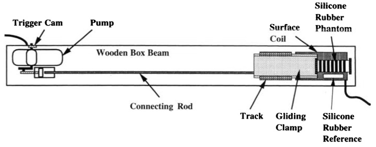
Phantom deformation apparatus. A respirator pump (left) cyclically moves a connecting rod and gliding clamp to deform the phantom (right). Black bands on the phantom allow photographic deformation measurement. The trigger cam generates a trigger every cycle to gate the imager and camera.

A respirator pump (model 607; Harvard Apparatus, South Natick, Mass) with an amplitude and frequency that were easily adjustable was bolted to the near end of the beam to produce a cyclical motion. At the far end, a fixed clamp was used to hold the far edge of the phantom. The phantom was suspended 2 mm over a standard 5 × 11-inch (12.5 cm × 27.5 cm) surface coil that was oriented lengthwise and fastened to the beam by wooden mount blocks. The near end of the phantom was clamped to a beveled Perspex glider that slid over Teflon-taped bearings in a Perspex track. The track was attached to the beam with brass screws. Finally, the near end of the glider was attached to the pump piston with a rigid, hollow aluminum tube (outside diameter, 1.9 cm; thickness, 1.6 mm). This was supported in the middle by a plastic bearing to damp bending oscillation.

To produce a gating trigger at a particular phase of the cycle, a cam was attached to the main axle of the pump, which depressed a microswitch connected to a 4.6-V battery.

Timing Circuitry

An electronic circuit was built to gate the imager, trigger the camera after a desired delay, and display the camera flash delay in the photographs (Fig 2). The circuit was built on a breadboard powered by four size D batteries connected in a series (6 V).

Figure 2.

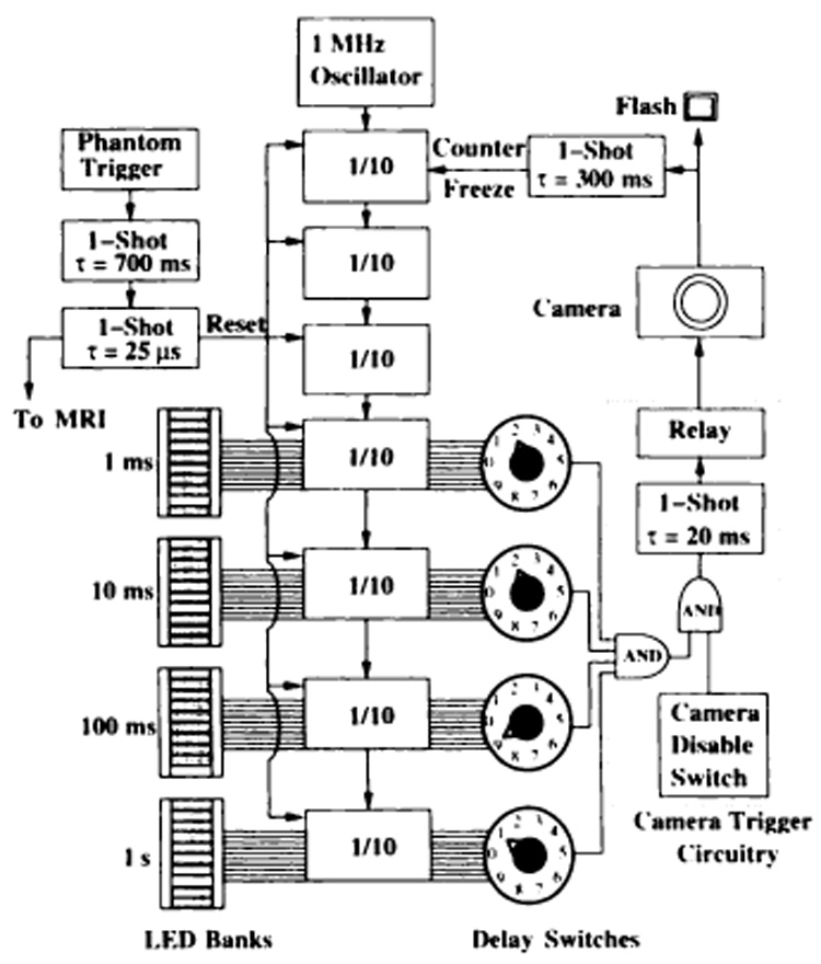
Timing circuitry. This circuit reads the phantom trigger, triggers the camera after a variable delay, displays the flash time in light-emitting diodes (LEDs), and sends a debounced gating trigger to the imager. The 1-MHz oscillator (top center) drives a cascade of divide-by-ten (1/10) integrated circuits (ICs) to form an LED timer. See text for details. MRI = MR imaging, ms = milliseconds, s = seconds.

First, the phantom trigger was debounced with a series of complementary metal-oxide semiconductor (CMOS) 4047 one-shot ICs. The first had a pulse duration of 700 msec to ensure that there could be only one trigger per cycle. This triggered a second one-shot IC with a short pulse duration of 25 µsec. This pulse was sent to the imager and to the clock reset in the timing circuit.

The timer consisted of a 1.000-MHz transistor-transistor logic oscillator (model F1100E; Fox Electronics, Fort Meyers, Fla) and a cascade of seven divide-by-tens (CMOS 4017). Each divide-by-ten had a reset input from the 25-µsec one-shot IC. A short output pulse from the second one-shot IC was necessary because the divide-by-tens reset the timer on the rising edge but do not begin counting until the falling edge. Outputs from each of the last four divide-by-tens went to a bank of 10 LEDs to display the time with a 1-msec resolution.

The same outputs also went to four 10-pole switches to form an adjustable camera trigger delay. Because the output of a switch was high only when the desired digit was active, their connection with a logical AND gate (CMOS 4081) produced a 1-msec pulse at the dialed delay. Next, this signal was combined in an AND gate with a manual disable switch so that the camera could be kept from firing at every cycle. Finally, this delayed pulse was lengthened by a 20-msec one-shot IC and sent to a relay (CMOS 4066) to short circuit the inputs to the camera shutter.

Since there was a variable delay (105–110 msec) between the triggering of the camera and the flash, the camera flash signal was used to stop the LEDs and display the exact delay in the photograph. Specifically, the 5-V flash wire from the camera was sent to a 300-msec one-shot IC. Its output was then sent to the "enable" pin of the first divide-by-ten to stop the clock from counting at the time of the flash and hold the clock fixed throughout the 1/30-second shutter time.

Experimental Protocol

The phantom trigger pulse was adjusted to occur 50 msec before the maximum contraction of the phantom, and the pump was set to 69 cycles per minute with a maximum displacement of 5.4 cm. These motions produced deformations that approximated those seen in the beating heart. The apparatus was allowed to stabilize for 30 minutes before the experiment and was kept running throughout the experiment.

A series of flash photographs with increasing delays was obtained with the apparatus on the floor of the examination room. The assembly was then loaded into the imager, and the MR images were obtained. In both cases, the apparatus was supported in an identical fashion to ensure that bending did not change the resting length of the phantom.

Photography

Photographs were obtained with a camera (model 8008; Nikon, Tokyo, Japan) equipped with a 105-mm 1.0:2.8 lens (model AF, Micro Nikkor; Nikon, Tokyo, Japan) and an SB23 Speedlight flash and black and white film (TMAX100; Eastman Kodak, Rochester, NY). The camera was mounted 1 m directly above the phantom, and the flash was 1.5 m above and 1 m to the side of the phantom. The flash angle reduced glare and allowed shielding of the bank of LEDs from the flash.

Figure 3 shows the deformation reference photograph of the phantom obtained 109 msec after the trigger. Next to the phantom, a bank of LEDs from the timing circuit was positioned to display the time of image flash, a ruler for absolute dimension reference, a fixed block of silicone rubber for image registration, and a digital watch for absolute time.

Figure 3.

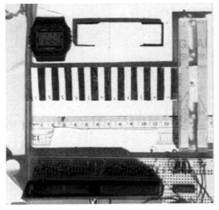
Reference photograph of the phantom. The photograph was digitized to define the undeformed phantom geometry. The phantom is in a horizontal position with vertical black bands. It was fixed at the left and cyclically pulled from the gliding clamp at the right. The LEDs are at the bottom. A digital watch and a fixed, rubber reference are above the phantom.

MR Tagging and Imaging

MR imaging was performed by means of a 1.5-T imager (Signa; GE Medical Systems, Milwaukee, Wis) with software release 4.7. A modified DANTE (delays alternating with nutations for tailored excitations)-spatial modulation of magnetization (SPAMM) parallel line tagging method was used, followed by a fractional-echo imaging sequence (2,3,5). The pulse sequence is shown in Figure 4. Frequency encoding was oriented along the direction of motion. The sequence was gated from the phantom trigger, and tagging occurred at maximal contraction. The imaging parameters were as follows: repetition time (TR), 8.40 msec; echo time (TE), 2.57 msec; field of view, 24 cm; eight excitations; 5° tip angle; 5-mm tag separation; 256 × 128 matrix; and a 180° tag inversion. Tag width and spacing were optimized to be approximately 1.5 and 7 pixels, respectively (10,11). Tag lines were perpendicular to the frequency encoding axis and the direction of phantom motion.

Figure 4.

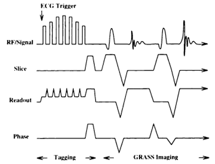
Tagging and imaging pulse sequence. A hybrid DANTE-SPAMM tagging sequence is followed by a fractional-echo sequence performed with gradient-recalled acquisition in the steady state (GRASS). The short echo time (2.57 msec) minimized motion artifact; the short repetition time (8.40 msec) enabled high time resolution. ECG = electrocardiographic, RF = radio frequency.

Figure 5a shows the reference MR image of the phantom obtained 109 msec after the trigger; Figure 5b, an image of the deformed phantom obtained 148 msec after the reference image was obtained. Next to the phantom in each case was the smaller, fixed rubber position marker. Tags in the marker remained at the original 5-mm spacing. The increase in tag spacing in the phantom shows the deformation (Fig 5).

Figure 5.

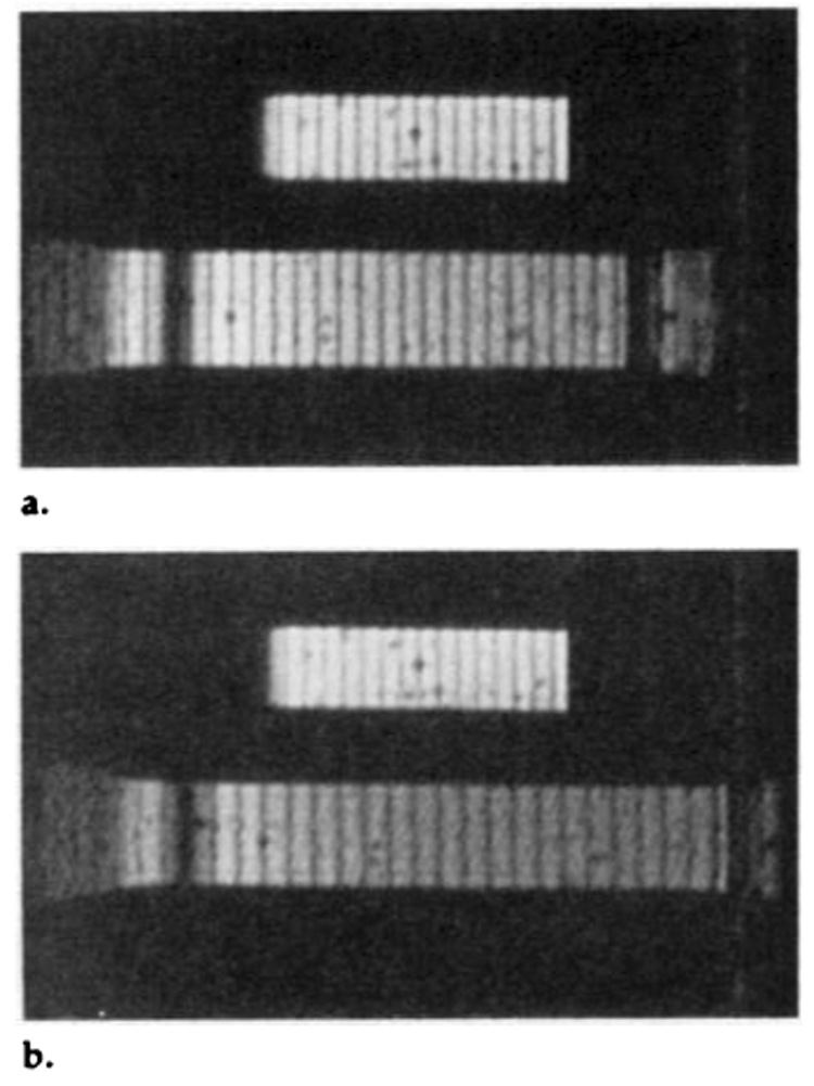
Reference and deformed MR images of the phantom. (a) Reference MR image of the phantom, which is fixed at the left and pulled from the right. Above is the smaller, fixed position reference. (b) MR image obtained 148 msec later. The increase in tag spacing in the phantom illustrates the deformation.

A schematic of the data acquisition timing is shown in Figure 6. The trigger of the phantom initiates either the photographic system or MR sequence. For photography, the delay dials in the timing circuit allowed camera triggering at different delays. Once triggered, the camera produced a flash 105–110 msec later. MR images were acquired after an imager delay, which positioned an image at the photographic reference time.

Figure 6.

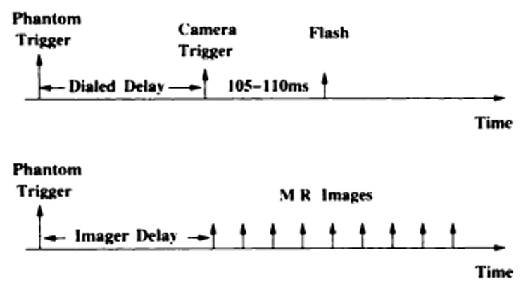
Data acquisition timing diagram. The trigger from the phantom initiates either MR imaging or photography. Top: To obtain a photograph, a delay is programmed to change the camera trigger time. After a camera delay of 105–110 msec (ms), the flash occurs to expose the phantom. Bottom: MR images are obtained in rapid succession after an imager delay.

Photographic Processing

The photographs of the phantom were converted to a compact disk format (PhotoCD; Eastman Kodak, Rochester, NY) by a photography laboratory outside our institution. A variety of resolution levels were available on the compact disk. The highest resolution digitization of the 35-mm negative was 3,072 × 2,048 pixels. A cropped image of the region of interest was read from the compact disk at 1,024 × 1,536 resolution as "gray scale" onto a personal computer (Macintosh; Apple Computer, Cupertino, Calif) with commercial software (PhotoEdge, Eastman Kodak).² These image files were read into an image analysis program (Image, version 1.47; W. Rasband, Research Services Branch, National Institute of Mental Health, National Institutes of Health, Bethesda, Md)³ as eight-bit images and displayed as gray scale. The profile function in the Image program was used to read pixel intensities through the center of the phantom. The profiles were saved to disk as ASCII (American Standard Code for Information Interchange) files.

These profiles were then used to estimate the position of the marked liners on the surface of the phantom. Figure 7 shows exemplary signal intensity profiles from the phantom at the reference time and 148 msec later. A high degree of accuracy was achieved in edge detection because there were at least four pixels across steep transitions.

Figure 7.

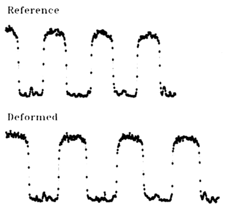
(7) Photographic pixel (■) profiles at reference time and 148 msec later (Deformed). The horizontal axis is the position along the phantom, and the vertical direction for each tracing represents pixel intensity. Deformation is evident from the increased separation of the vertical edges. The valleys represent the black bands on the white rubber.

The spatial resolution of the photographs was measured from the image of the reference grid to be 0.420 mm ± 0.001 (standard deviation [SD]) per pixel, or approximately 2.5 pixels per millimeter. The computed contrast-to-noise ratio (C/N) between the black lines and the white rubber was approximately 23. This was lower than anticipated. To increase the S/N of the profiles, four adjacent pixel rows were averaged into each profile. The C/N improved to approximately 46.

Fourier filtering was used to determine the edge positions from the profiles. Specifically, a MATLAB (Math Works, Natick, Mass) function was written that performed the following steps:

(a) Fourier transform the 512-point profile, (b) multiply the transform of the profile with the transform of an edge kernel, (c) zero fill the Fourier data to 8,192 points to decrease the pixel spacing in the filtered profile for subpixel position estimation, (d) apply the inverse Fourier transform to the zero-filled data, (e) search the filtered data for local extrema, and (f) record the location of the local extrema as "edge coordinates."

All data that corresponded to the central 7 cm of the undeformed phantom were used in subsequent analyses. This region of the phantom was chosen because it was far from the clamps that alter the deformation locally.

There was no need to register the photographic data over different time points because only relative positions of the edges were used in the deformation analysis.

MR Image Processing

MR images were converted to 16-bit files for processing. Profiles through the center of the MR image that were perpendicular to the tags were used as input to the MATLAB tag detection program. Figure 8 shows exemplary signal intensity profiles from the phantom at the reference time and 148 msec later. This is the MR imaging analog to Figure 7.

Figure 8.

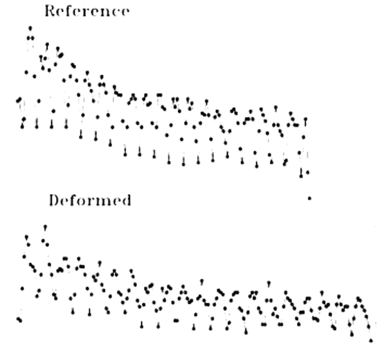
(8) MR imaging pixel profiles at reference time and 148 msec later (Deformed). The horizontal axis is the position along the phantom, and the vertical direction for each tracing represents pixel intensity. Deformation is evident from the increased separation of the tag minima. Lower tag amplitudes in the deformed image result from tag fading.

The S/N of the raw images ranged from 18 ± 4 at the reference image (109-msec delay) to 10 ± 0.5 at the last image analyzed (251-msec delay). Profile S/N of the MR imaging data was doubled by averaging four adjacent rows of pixels together, as was done for the photographs. The position of each tag was estimated with the same Fourier filtering technique described above, but a Gaussian tag model was used as the filter kernel.

RESULTS

Deformation from Photographic Data

Figure 9 shows the position of the marker edges at four time points as a function of their position at the reference time frame. The slope of the line fitting these points is the deformation of the phantom. A linear fit was used because the deformation was expected to be uniform over the length of the phantom used in this analysis. This slope was used as the "true" deformation for validating that from MR imaging. The Table gives the value of the deformation calculated with this method at four time points. The standard errors in these values were all less than 0.001.

Figure 9.

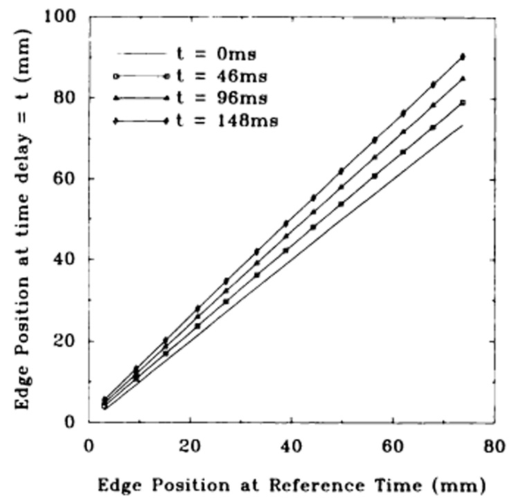
(9) Position of photographic edges versus initial position at reference time. Three time curves are shown in addition to the reference curve at 0 msec, which has unity slope by definition. The slope indicates the deformation. The standard errors in position about the linear fits were, respectively, 0.025 mm, 0.060 mm, and 0.082 mm for the 46-, 96-, and 148-msec curves. In 9–11, ms = milliseconds; in 9 and 10, t = time.

Time versus Deformation for the Photographic Data for Four Time Delays after the Trigger Pulse

Time (msec)	Deformation	Standard Error †
109 ± 0.5*	1.000	0.0
155 ± 0.5	1.0649	0.00028
205 ± 0.5	1.1356	0.00069
257 ± 0.5	1.2022	0.00098

^*The image obtained at a 109-msec delay is used as the reference image for the deformation calculations.

^†The standard error is estimated from the scatter of individual marker edge positions about a linear fit versus initial edge position.

Deformation from MR Imaging Data

The MR image at the trigger delay of 109 msec was the reference image for calculation of the deformation of the phantom, because it matched the delay of the photographic reference. Seventeen MR images were obtained in the interval between the four photographs. Figure 10 shows the position of the tags in the phantom at four time points as a function of their initial position at the reference time. The slopes of linear fits to these points are the deformations as calculated from the MR imaging data. The standard errors of the slope estimates increased with time because the C/N between tags and background rubber decreased as the magnetization approached steady state.

Figure 10.

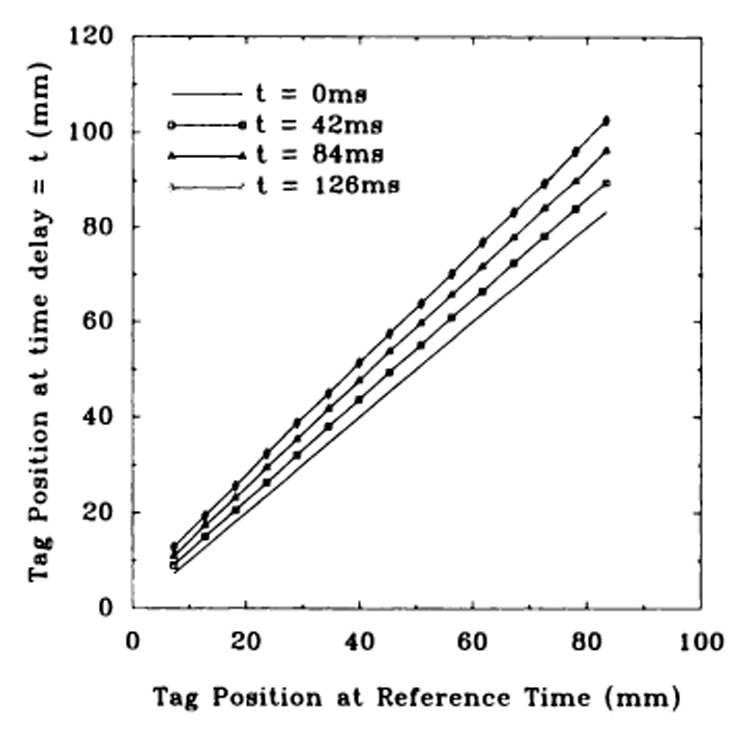
(10) Position of MR tags versus initial position at reference time. Three time curves are shown in addition to the reference line at 0 msec, which has unity slope by definition. The slope indicates the deformation. The standard errors in position about the linear fits were, respectively, 0.090 mm, 0.150 mm, and 0.185 mm for the 42-, 84-, and 126-msec curves. Tag fading produces greater uncertainty in tag position with time.

Comparison of MR Imaging Data with Photographic Data

Figure 11 shows the deformation as a function of time for photographic and MR imaging data.

Figure 11.

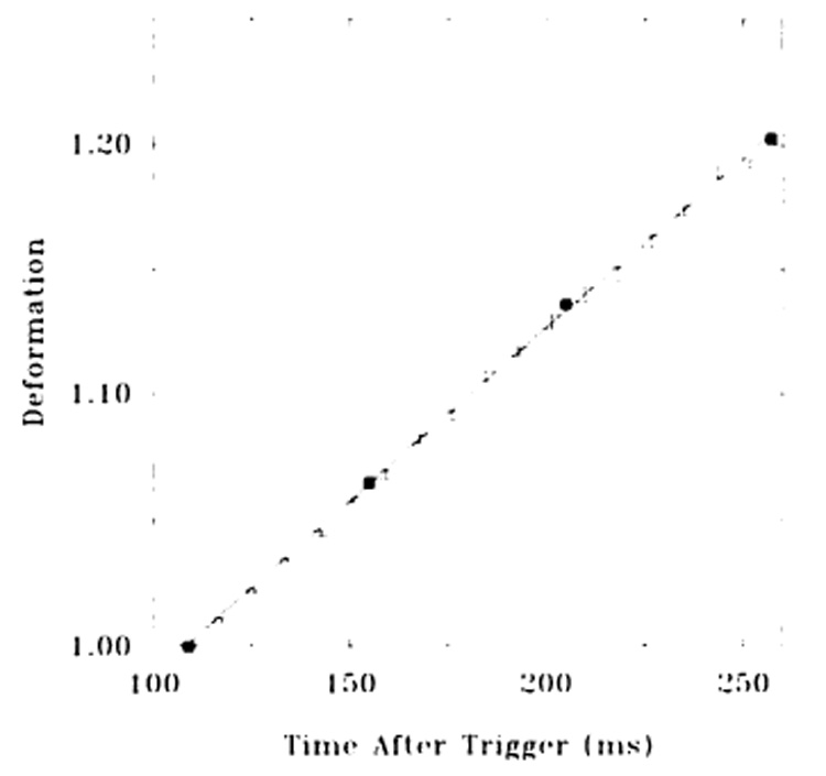
(11) Deformation versus time for photographic and MR imaging methods. The photographic data are shown as solid squares, and a linear regression line through them is also shown. MR data are shown as points with symmetric error bars. Error bars show the standard errors in the slopes of tag-position versus reference-tag-position lines, as shown in 10.

The uncertainty of the photographic deformation points was less than 0.1%. The deformations (F) of these four photographic points were fit by a straight line as a function of time (t), in seconds: F = 1.375(t) + 0.8514. The SD about this line was 0.0025. This line is also shown in Figure 11. While the motion of the phantom was not linear over the entire elongation, over the time interval of 109 to 257 msec after the trigger, the motion was well approximated with a linear fit. An analytical solution of the motion was unreliable because the motion depended on the cyclic loading of the motor, which changed as the phantom was stretched.

The SD of the MR imaging data about the line was 0.002. This was approximately equal to the standard error in the linear fits to the MR imaging data.

DISCUSSION

The small scatter (0.002 SD) of the MR imaging data over the photographic data indicated a high precision and accuracy in the MR imaging deformation measurements. This agreement of the compact disk and the MR imaging was achieved even with two known sources of error.

The linear fit to the four photographic data points was an approximation, and most of the error in this fit was not due to noise in the data but to the approximation of the linear model. Another source of error in the analysis was the fact that the time delays of the reference images could only be matched to within 1 msec. This was probably the cause of the bias of the MR imaging data toward the lower deformation values presented in Figure 11.

This analysis was performed with very low S/N data for MR imaging. Therefore, the calculated accuracy and precision are lower bounds for the performance of the method in other phantoms in which imaging properties more closely resemble those of myocardium (8,9). Less pixel averaging would be necessary in images with a higher S/N and thus would enable higher spatial resolution of the deformation estimates.

This particular MR pulse sequence was chosen for the standard because it was also designed for cardiac imaging; however, the parameters that were used made the imaging time too long for breath-hold imaging. The parameters were designed to produce high temporal resolution, high spatial resolution, and an adequate S/N, to provide the best deformation estimates.

The MR standard sequence was evaluated for one-dimensional deformations from motion that were primarily along the readout direction. This MR pulse sequence can be used in such a phantom to evaluate and optimize the ability of any other sequence used to measure one-dimensional deformations. Under the assumption that three-dimensional deformations can be reconstructed from orthogonal one-dimensional data with sufficient sampling density, the method is useful for evaluation of sequences designed for measurement of three-dimensional deformations.

The advantage of having an MR imaging tagging standard is that spatial and temporal registration between any new method being tested and the MR standard is very simple. In addition, experiments can be performed in phantom materials in which MR properties and geometries more closely match those of the heart; therefore, one can avoid all the material property and geometric restrictions of a phantom that can be photographed.

Previous reports showed that tags could be detected in stationary phantoms (10) and rigid rotation phantoms (7) with high accuracy. We have now validated the use of tagging for motion measurement in a phantom undergoing deformations that are at the same rate and magnitude as those found in the heart. The validated tagging method can now be used as the standard to evaluate other MR imaging motion estimation techniques.

Abbreviations

C/N

contrast-to-noise ratio

IC

integrated circuit

LED

light-emitting diode

SD

standard deviation

S/N

signal-to-noise ratio

SPAMM

spatial modulation of magnetization

TE

echo time

TR

repetition time

References

- 1.Zerhouni EA, Parish DM, Rogers WJ, Yang A, Shapiro EP. Human heart: tagging with MR imaging—a method for noninvasive assessment of myocardial motion. Radiology. 1988;169:59–63. doi: 10.1148/radiology.169.1.3420283. [DOI] [PubMed] [Google Scholar]
- 2.Mosher TJ, Smith MB. A DANTE tagging sequence for the evaluation of translational sample motion. Magn Reson Med. 1990;15:334–339. doi: 10.1002/mrm.1910150215. [DOI] [PubMed] [Google Scholar]
- 3.Axel L, Dougherty L. MR imaging of motion with spatial modulation of magnetization. Radiology. 1989;171:841–849. doi: 10.1148/radiology.171.3.2717762. [DOI] [PubMed] [Google Scholar]
- 4.Bolster BD, McVeigh ER, Zerhouni EA. Myocardial tagging in polar coordinates with use of striped tags. Radiology. 1990;177:769–772. doi: 10.1148/radiology.177.3.2243987. [DOI] [PMC free article] [PubMed] [Google Scholar]
- 5.McVeigh ER, Atalar E. Cardiac tagging with breath hold CINE MRI. Magn Reson Med. 1992;28:318–327. doi: 10.1002/mrm.1910280214. [DOI] [PMC free article] [PubMed] [Google Scholar]
- 6.Fischer SE, McKinnon GC, Maier SE, Boesigner P. Improved myocardial tagging contrast. Magn Reson Med. 1993;30:191–200. doi: 10.1002/mrm.1910300207. [DOI] [PubMed] [Google Scholar]
- 7.McVeigh ER, Zerhouni EA. Noninvasive measurement of transmural gradients in myocardial strain with MR imaging. Radiology. 1991;180:677–683. doi: 10.1148/radiology.180.3.1871278. [DOI] [PMC free article] [PubMed] [Google Scholar]
- 8.Young AA, Axel L, Dougherty L, Bogen DK, Parenteau CS. Validation of tagging with MR imaging to estimate material deformation. Radiology. 1993;188:101–108. doi: 10.1148/radiology.188.1.8511281. [DOI] [PubMed] [Google Scholar]
- 9.Goldstein DC, Kundel HL, Daube-Witherspoon ME, Thibault LE, Goldstein EJ. A silicone get phantom suitable for multimodality imaging. Invest Radiol. 1987;122:153–157. doi: 10.1097/00004424-198702000-00013. [DOI] [PubMed] [Google Scholar]
- 10.Atalar E, McVeigh ER. Optimization of tag thickness for measuring of position with magnetic resonance imaging. IEEE Trans Med Imaging. doi: 10.1109/42.276154. (in press) [DOI] [PMC free article] [PubMed] [Google Scholar]
- 11.McVeigh ER, Gao L. Book of abstracts: Society of Magnetic Resonance in Medicine 1993. Vol. 199. Berkeley, Calif: Society of Magnetic Resonance in Medicine; 1993. Precision of tag position estimation in breath-hold CINE MRI: the effect of tag spacing (abstr) [Google Scholar]