

Abstract
PURPOSE
To present a database of systolic three-dimensional (3D) strain evolution throughout the normal left ventricle (LV) in humans.
MATERIALS AND METHODS
In 31 healthy volunteers, magnetic resonance (MR) tissue tagging and breath-hold MR imaging were used to generate and then detect the motion of transient fiducial markers (ie, tags) in the heart every 32 msec. Strain and motion were calculated from a 3D displacement field that was fit to the tag data. Special indexes of contraction and thickening that were based on multiple strain components also were evaluated.
RESULTS
The temporal evolution of local strains was linear during the first half of systole. The peak shortening and thickening strain components were typically greatest in the anterolateral wall, increased toward the apex, and increased toward the endocardium. Shears and displacements were more spatially variable. The two specialized indexes of contraction and thickening had higher measurement precision and tighter normal ranges than did the traditional strain components.
CONCLUSION
In this study, the authors noninvasively characterized the normal systolic ranges of 3D displacement and strain evolution throughout the human LV. Comparison against this multidimensional database may permit sensitive detection of systolic LV dysfunction.
Previous methods for cardiac strain measurement in humans have been limited by low spatial resolution or invasiveness. Coronary arterial bifurcations have been tracked in three dimensions with cine radiography (1,2). In the transplanted human heart, the motion of metal markers implanted near the midwall, as detected by using biplanar cine radiography, also has been used to calculate strain (3-7).
Magnetic resonance (MR) tissue tagging (8-14) with dynamic MR imaging is a rapidly developing technique for the quantitative, noninvasive evaluation of cardiac mechanical function with high spatial and temporal resolution. Tags are regions, usually planes, of tissue in which the magnetization is altered by special MR pulses. Differences in signal intensity between tagged regions and undisturbed regions serve as a means of accurately tracking the motion of the underlying tissue on subsequent MR images (15-18). Mathematical techniques are then used to reconstruct a three-dimensional (3D) deformity from tag positions on cine MR images (19-22).
The normal pattern of 3D strain evolution in the human left ventricle (LV) has been only grossly characterized. The purpose of this work was to determine the normal range of 3D systolic displacement and strain as a function of position in the LV and of time during systole. This database is needed as a reference with which strains in abnormal hearts can be compared. It could also be used to test current models of cardiac mechanics, quantify degrees of function during stress testing, or quantify degrees of contraction asynschrony in paced hearts or hearts with conduction anomalies.
MATERIALS AND METHODS
Thirty-one healthy volunteers who gave informed consent were examined; these individuals had no clinical history of cardiovascular disease, diabetes mellitus, or potential cardiac symptoms such as chest pain or dyspnea. The volunteers were predominantly white, and there was a nearly even distribution of men and women (16 men, 15 women; mean age ± SD, 37 years ± 11; age range, 21–62 years). The age, sex, race, and heart rate of the volunteers are listed in Table 1. The study was approved by to Joint Committee on Clinical Investigation and was carried out in accordance with institutional guidelines.
TABLE 1.
Patient Demographic Data
| Volunteer
No. |
Age | Sex | Race | Heart Rate
(bpm)* |
|---|---|---|---|---|
| 1 | 29 | M | White | 68 |
| 2 | 29 | F | White | 73 |
| 3 | 28 | M | White | 58 |
| 4 | 30 | F | White | 60 |
| 5† | 27 | M | White | 50 |
| 6† | 30 | M | White | 45 |
| 7 | 47 | F | White | 67 |
| 8 | 31 | M | White | 76 |
| 9 | 47 | F | White | 67 |
| 10 | 25 | M | White | 56 |
| 11 | 35 | F | White | 61 |
| 12 | 57 | M | White | 77 |
| 13 | 62 | M | White | 56 |
| 14 | 52 | M | White | 62 |
| 15 | 30 | F | White | 69 |
| 16 | 26 | M | White | 60 |
| 17 | 30 | F | White | 83 |
| 18 | 31 | M | White | 68 |
| 19 | 25 | F | White | 64 |
| 20 | 28 | M | Asian | 75 |
| 21 | 21 | M | Asian | 72 |
| 22 | 50 | F | White | 59 |
| 23 | 51 | M | White | 96 |
| 24 | 41 | F | White | 76 |
| 25 | 55 | F | Asian | 54 |
| 26 | 38 | F | White | 69 |
| 27 | 44 | F | White | 75 |
| 28 | 31 | F | White | 72 |
| 29 | 50 | M | White | 69 |
| 30 | 44 | F | White | 84 |
| 31 | 28 | M | White | 90 |
Data are the heart rate during MR imaging.
Volunteers 5 and 6 were athletic men with resting heart rates typically in the upper and lower 50s, respectively.
MR Imaging
MR imaging was performed, with the volunteers in the supine position, by using a Signa 1.5-T imaging unit (GE Medical Systems, Milwaukee, Wis) with a flexible surface coil wrapped around the left side of the chest. A cardiac-gated (upslope of the electrocardiograph R wave) pulse sequence with parallel plane tagging (14,23) and blood saturation (24) was used during breath holds, in 22 heart beats, at end-expiratory lung volume to rapidly acquire tagged images with minimal motion artifact. The tagging sequence consisted of five nonselective radio-frequency pulses with relative amplitudes of 0.7, 0.9, 1.0, 0.9, and 0.7 separated by gradient pulses to achieve a tag spacing of approximately 6 mm. The tagging tip angle was tuned to 180°. The center of the tagging pulse occurred 20 msec after the trigger, and this was considered to be the end-diastolic reference time. MR imaging involved spoiled gradient-recalled acquisition at steady state with k-space segmentation and a partial echo to minimize imaging time.
Three sets of tagged MR images with 32.5-msec temporal resolution we acquired in each heart. There were two sets of six parallel, short-axis sections with orthogonal tags and one radially oriented set of six long-axis sections spaced every 30° with tags perpendicular to the long axis. Representative short- and long-axis images at early, middle, and late systole are shown in Figure 1 to illustrate the image and tag orientation and the ability of tags to depict the underlying myocardial deformity. The top row shows a basal short-axis section at three phases of contraction. The section (middle) row is analogous to the first, but the tags and readout gradient have been rotated 90°. The bottom row shows a long-axis section at the same three times through systole.
Figure 1.
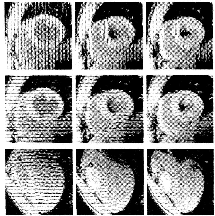
Early (28 msec) (left), middle (188 msec) (middle), and late (351 msec) (right) systolic tagged MR images in a normal human heart. The top and middle rows show a basal short-axis section with different tag orientations, and the bottom row shows a long-axis section. Tag motion, as seen on these images, provides three orthogonal sets of one-dimensional displacement information throughout the heart wall.
The MR imaging parameters for each section were as follows: 6.5/2.1 (repetition time msec/echo time |fractional echo| msec), 36-cm field of view, 12° flip angle, 110 phase-encoding steps (256 × 110 matrix), ±32-kHz bandwidth, one signal acquired, and five phase-encoding views per time frame. Each cine MR sequence included nine to 12 images.
Strain Calculation
The images were processed by using semiautomated software (25) to identify the tag lines within the myocardium and the endocardial and epicardial contours. All hearts were registered about the long axis by aligning the major axes of prolate spheroids that were fit, with least-squares minimization, to the epicardial contours of each LV. Next, the midpoints of the basal right ventricular insertions were aligned. A standardized, regularly spaced material point array (ie, sample points within the myocardium where the positions and strains were tracked three dimensionally) was defined in each normal heart. Short-axis planes of material points, called levels, were defined at regular percentages of the distances between the LV apical point and the basal valve plane within the volume spanned on the short-axis images. Because of variation in short-axis imaging geometry, not all apical and basal levels were present in all the hearts. Within a level, material points were spaced at even angles (ie, sectors) about the long axis at the endocardium, midwall, and epicardium. Thus, anatomically corresponding material point positions were defined in each LV.
Three-dimensional displacements and strains were determined at each material point by using the displacement field fitting method (21). Each time frame was reconstructed independently and based solely on tag positions, which are more precisely identified than the cardiac contours (26). All the one-dimensional displacement data from the three sets of images with orthogonal tag planes (approximately 2,400 points per time frame) were simultaneously fit to a 3D displacement function by using a least-squares methods. This function included 12 first-order Cartesian terms describing bulk motion and spatially invariant shears and stretches, followed by a 150-term harmonic expansion in prolate spheroidal coordinated to fit higher modes of local displacement variation. The prolate spheroidal expansion contained first-order terms In the radial direction and fourth-order terms in the circumferential and longitudinal angles (see Appendix A) (21). Spatial gradients of this displacement function were used to calculate the Lagrangian finite deformation gradient tensor F at the material points in the heart wall.
Strain and displacement at each material point were expressed in a local coordinate system along the radial, circumferential, and longitudinal directions, on the basis of the orientation of the overlying epicardial surface at the reference (undeformed) geometry. These relationships are shown in Figure 2 (A). The radial direction was outward and perpendicular to the epicardial surface. The circumferential direction was In the short-axis plane (perpendicular to the long axis), parallel to the epicardial surface, and counterclockwise, as viewed from the base. The longitudinal direction was in the plane defined by the material point and the long-axis line, tangent to the epicardial surface, and increased from the apex to the base. Thus, various radial-circumferential longitudinal coordinate angles and planes were defined to create a right-handed system. The angles between pairs of these coordinate directions, which are illustrated in Figure 2 (B), were used to describe the orientations of the principal strains.
Figure 2. Local coordinate systems and angles.
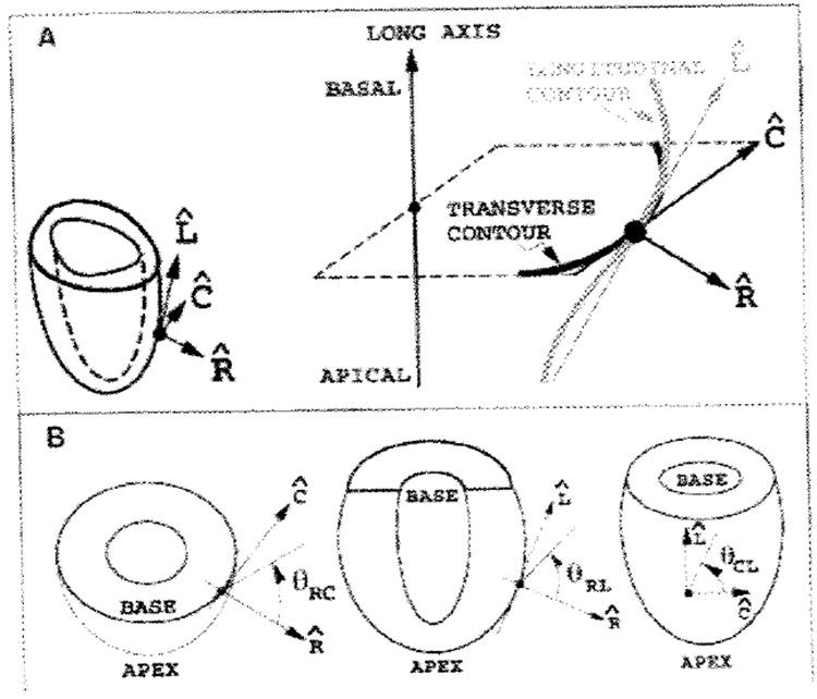
In diagram A, a separate cartesian coordinate system, in which the axes are radial , circumferential , and longitudinal , is defined for each material point. The material point is projected along the prolate radial direction to the epicardium, where the coordinate directions are determined. The local coordinate system is detailed to the right. is the epicardial outward normal vector, which is normal to the heart contours in transverse and longitudinal sections. is the cross product of the long axis with which ensures that lies In the transverse plane. is the cross product of , which lies in the longitudinal plane. Diagram B shows the angles used to describe principal strain directions. At left, the angle in the plane (θRC) and is measured from to ; similar definitions for plane (θRL) and plane (θCL) are shown in the middle and left drawings, respectively.
The Lagrangian finite strain tensor E was calculated from the relationship E = ½FTF − I, where the superscript T represents the matrix transpose, and I, the identity tensor. Polar decomposition of F gave the right stretch tensor U, where F equals RU, and R is a bulk rotation matrix.
A shortening Index (SI) was defined to reflect the geometric mean of fractional one-dimensional shortening within the circumferential-longitudinal plane. The SI is negative for muscle shortening in any direction that produces a net area decrease in this plane. This parameter is directionally insensitive within the plane and therefore a robust way to report myocardial contraction. Mathematically. it is the square root of the fractional area change in the plane minus 1.0, so that it is zero with no strain (see Appendix B for derivation), which is expressed as follows:
| (1) |
where × represents the vector cross product; the vertical bars represent the vector magnitude; and the subscripts RC, CC, LC, RL, CL, and LL represent, respectively, the radial-circumferential, circumferential, longitudinal-circumferential, radial-longitudinal, circumferential-longitudinal, and longitudinal components of U. The same-letter subscripts (ie, CC and LL) denote length changes along that coordinate direction and are associated with axial strains. (In continuum mechanics, this is usually called “normal strain”; however, this nomenclature would be confusing in this article.) The different-letter subscripts (ie, RC, LC, RL, and CL) refer to shear within the plane defined by the two coordinate directions. Various normal and abnormal deformations and the associated SI values are illustrated in Figure 3. For contraction of the wall, the SI is negative, and for stretching of the wall, it is positive. Circumferential and longitudinal contractions contribute equally to the SI, and simple shear in the circumferential-longitudinal plane has no effect.
Figure 3. Examples of SI deformations.
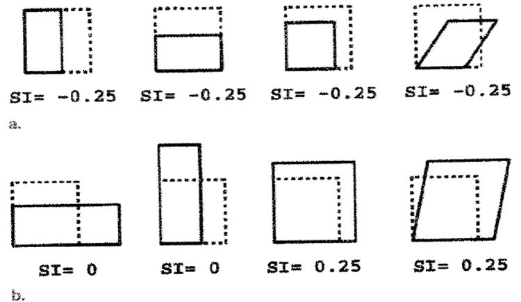
The area inside the dashed lines represents the undeformed state within the plane. (a) Various contractions, all of which have area decreases (44%) that correspond to SI values of −0.25. With uniform contraction (3rd from left), both of the deformed edges, which reflect geometric mean shortening, are 25% shorter. (b) Abnormal deformations. No mean shortening or area change is seen in the two left panels, and increases ate seen in the two right panels.
By using the assumption of tissue incompressibility, a wall thickening parameter T, which is an estimation of the local fractional thickening at a material point, also was calculated. This parameter was supported by a high spatial density of tag data and also allowed for a more direct comparison with traditional wall thickening than can be done with radial strain ERR, which is a nonlinear function of fractional length change. Fractional length change is expressed as (2E + 1)½ − 1, where E is the axial strain component along the desired direction. Incompressibility was enforced by setting the determinate of U to equal 1.0 after replacing the radial component of the right stretch tensor URR with (T + 1) and solving for T (see Appendix C for derivation) as follows:
| (2) |
The rotation and torsion of the LV about its long axis also were evaluated. The rotation of a material point was calculated about the centroid of the short-axis plane that contained that point so the bulk translation would not produce artifactual variations in the calculated rotation. Following the coordinate system illustrated in Figure 2, positive angles were defined counterclockwise, as viewed from the base. Torsion, which is the long-axis gradient of rotation, was calculated by using the average rotation of material points at each level. Following the work of other authors (27-30), as well as the sign convention in Figure 2, we defined torsion angles relative to the basal (81%) level, with positive values representing relative clockwise rotation of more apical levels, as viewed from the base.
The duration of local systole at each material point was defined for each strain component as the time to the maximum strain magnitude, or the peak strain. The average systolic strain evolution was then calculated by including strain data through local end systole. At a given material point position, different hearts reached a peak strain at different times. Thus, when the strains of hearts were averaged at each time frame, for the later time frames, there were fewer hearts that contributed systolic strain data. The average strain at a material point was calculated if five or more hearts remained in local systole at that time. Adjustment for heart rate before averaging among hearts was not performed because it would have introduced an additional postprocessing step with its own variability and was not found to narrow the range of normal strain. For displacement and rotation, local end systole was defined as the time of greatest principal contraction, because these parameters were not monotonic.
Statistical Analysis
Statistical analysis for the spatial variation of strain or displacement at the midwall was performed with repeated measures analysis of variance (two-way) by using STATISTICA software (StatSoft, Tulsa, Okla). For midwall analyses, three levels—30%, 55%, and 80%—and four circumferential sectors—anterior, lateral, inferior, and septal—were used to limit the number of possible comparisons. If statistically significant variation was found, Scheffé subtesting was used to compare sectors, levels, or individual positions. For radial gradients, paired Student t testing was used to evaluate differences between the endocardium and epicardium at each circumferential-longitudinal position. A P value of .05 or less was considered to be significant.
RESULTS
Midwall Axial Strains and Indexes
The monotonic time courses of all axial strain parameters were observed during systole. The axial strain evolution curves for the 31 hearts were tightly clustered in each region throughout the LV, without outlying curves, although different hearts reached a peak strain at different times.
The average strain at each time frame during systole was calculated for the 31 hearts. A full-resolution strain map of the average SI evolution is shown in Figure 4a. Each box represents a different circumferential-longitudinal position for a midwall material point, and the SI versus time is plotted in each box. The mean and two 2-SD curves, calculated by averaging the heart strains at each time frame, are shown. The number of hearts with data at the different levels is shown to the right of each row. In addition, the mean and 2-SD values for the peak strain are shown as short horizontal lines at the left in each box. The values in this figure demonstrate the tight normal ranges, spatial heterogeneity, and smooth evolution of the SI parameter. The mean and SD of the peak SI, wall thickening, and axial strain components are listed In Table 2. Figure 4b shows renderings of a LV material point wire frame, with color encoding of the SI at the first, fourth, seventh, and 10th time frames. The LV is viewed from the apex, with the septum to the left (green dot). The colors range from yellow at no strain (SI = 0.0) to blue at 25% strain in-plane contraction (SI = −.25). The peak SI was greatest in magnitude apically (P < .001 vs equatorially or basally) and anteriorly and laterally (P < .005 vs inferiorly or at septal walls). The maximum mean SI magnitude (−0.25 ± 0.05) was at the apical anterior and lateral positions, and the minimum mean SI magnitude (−0.17 ± 0.03) was at the basal and equatorial portions of the septum (P < .001).
Figure 4. Average SI at midwall.
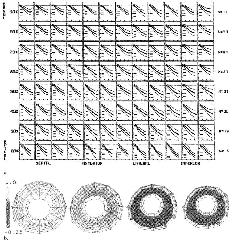
(a) Each box represents a midwall material point, with longitudinal levels from 20% to 90% of the distance from the apex to the base, and circumferential sectors spaced from the left to the right, as labeled. The number of hearts averaged (N)at each level is shown on the right. Within each box, the evolution of the SI, with the mean (thick middle line) and both 2-SD (thin outer lines) lines, are shown. The short horizontal lines at the left in each box represent the mean and 2-SD values of the peak SI. The horizontal ticks are spaced every 100 msec, and the vertical ticks are spaced every 0.1. (b) Three-dimensional renderings of the LV viewed from the apex. The middle of the septum (green dot) is on the left. The wire frame of all material points is shown at 46 msec, 143 msec, 241 msec, and 338 msec, with the midwall surface colored according to the value of the average SI. Tight normal ranges with smooth evolution are seen throughout the left ventricle with the SI.
TABLE 2.
Average Peak Strain Components and Indexes
| Strain | Septal | Anterior | Lateral | Inferior |
|---|---|---|---|---|
| SI | ||||
| Basal | −0.17 ± 0.03 | −0.20 ± 0.03 | −0.20 ± 0.03 | −0.18 ± 0.03 |
| Equatorial | −0.17 ± 0.03 | −0.22 ± 0.04 | −0.21 ± 0.03 | −0.18 ± 0.04 |
| Apical | −0.20 ± 0.03 | −0.25 ± 0.05 | −0.25 ± 0.04 | −0.24 ± 0.05 |
| T | ||||
| Basal | 0.46 ± 0.10 | 0.58 ± 0.12 | 0.60 ± 0.12 | 0.50 ± 0.11 |
| Equatorial | 0.49 ± 0.10 | 0.68 ± 0.17 | 0.61 ± 0.12 | 0.51 ± 0.14 |
| Apical | 0.63 ± 0.14 | 0.82 ± 0.21 | 0.80 ± 0.17 | 0.77 ± 0.20 |
| ERR | ||||
| Basal | 0.45 ± 0.12 | 0.42 ± 0.21 | 0.52 ± 0.19 | 0.41 ± 0.17 |
| Equatorial | 0.42 ± 0.19 | 0.52 ± 0.25 | 0.38 ± 0.18 | 0.35 ± 0.22 |
| Apical | 0.36 ± 0.22 | 0.67 ± 0.31 | 0.49 ± 0.29 | 0.39 ± 0.38 |
| ECC | ||||
| Basal | −0.17 ± 0.03 | −0.20 ± 0.03 | −0.21 ± 0.03 | −0.16 ± 0.03 |
| Equatorial | −0.16 ± 0.03 | −0.23 ± 0.04 | −0.22 ± 0.03 | −0.16 ± 0.05 |
| Apical | −0.18 ± 0.03 | −0.24 ± 0.06 | −0.24 ± 0.04 | −0.23 ± 0.04 |
| ELL | ||||
| Basal | −0.14 ± 0.03 | −0.15 ± 0.03 | −0.15 ± 0.03 | −0.15 ± 0.03 |
| Equatorial | −0.15 ± 0.03 | −0.15 ± 0.03 | −0.14 ± 0.04 | −0.15 ± 0.03 |
| Apical | −0.18 ± 0.04 | −0.19 ± 0.03 | −0.19 ± 0.03 | −0.18 ± 0.04 |
| ERC | ||||
| Basal | −0.01 ± 0.06 | 0.05 ± 0.06 | 0.05 ± 0.07 | 0.01 ± 0.08 |
| Equatorial | 0.02 ± 0.08 | 0.09 ± 0.06 | 0.05 ± 0.06 | 0.05 ± 0.07 |
| Apical | 0.11 ± 0.10 | 0.09 ± 0.09 | 0.05 ± 0.08 | 0.06 ± 0.08 |
| ERL | ||||
| Basal | 0.03 ± 0.09 | −0.05 ± 0.05 | 0.05 ± 0.07 | 0.01 ± 0.10 |
| Equatorial | 0.08 ± 0.05 | 0.01 ± 0.08 | 0.07 ± 0.06 | 0.03 ± 0.08 |
| Apical | 0.06 ± 0.09 | 0.02 ± 0.11 | 0.05 ± 0.08 | 0.09 ± 0.10 |
| ECL | ||||
| Basal | 0.01 ± 0.05 | 0.01 ± 0.04 | 0.03 ± 0.05 | 0.05 ± 0.05 |
| Equatorial | 0.03 ± 0.05 | 0.03 ± 0.03 | 0.03 ± 0.04 | 0.05 ± 0.04 |
| Apical | 0.04 ± 0.05 | 0.04 ± 0.04 | 0.04 ± 0.03 | 0.03 ± 0.04 |
Note.—Data are the mean ± SD. Basal values were at 80% of the distance from the apex to the valve plane; equatorial values, at 55%; and apical values, at 30%. The axial parameters tended to be greatest in the anterior and lateral walls. The ERR had the highest variability. ECC = circumferential strain, ECL = circumferential-longitudinal shear, ELL = longitudinal strain, ERC = radial-circumferential shear, ERL = radial-longitudinal shear.
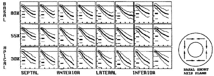
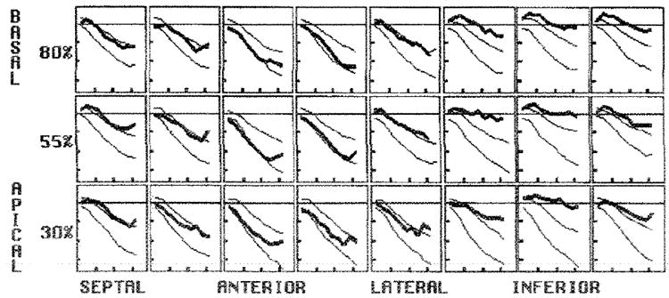
The local wall thickening at midwall is illustrated in Figure 5. A standard resolution array, which had data from 19 hearts at the 30% level, 31 hearts at the 55% level, and 29 hearts at the 80% level, is shown. This parameter had good precision, narrow 2-SD curves, and spatial heterogeneity. Similar to the SI, the wall thickening was greatest apically (P < .001 vs equatorially or basally) and anteriorly and laterally (P < .002 vs inferiorly or at septal walls). The extreme mean values were 0.82 ± 0.21 in the apical-anterior region and 0.46 ± 0.10 in the basal septum (P < .001). A plot of the directly calculated ERR is not shown because it had a lower measurement precision than did the local wall thickening.
Figure 5. Average midwall thickening parameter.
The circumferential sector changes are illustrated in each box, from the left to the right, and the longitudinal level varies from the top row (basal) to the bottom row (apical). In each box, the evolution curves are shown as the mean (thick middle line) ± 2 SDs (thin outer lines). The short horizontal lines at the left in each box represent the mean and 2-SD peak values. The vertical ticks are spaced every 0.4, and the horizontal ticks are spaced every 100 msec. A schematic drawing of wall thickening is on the right. Tight normal ranges with smooth evolution and spatial heterogeneity were seen throughout the LV with the wall thickening parameter.
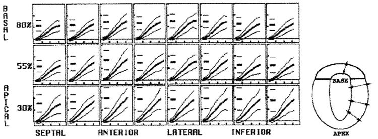
The evolution of the ECC at midwall is illustrated in Figure 6. This parameter also had tight SDs among the hearts; these values were typically less than 25% of the mean peak strain value. The ECC magnitude also was greatest apically (P < .001 vs equatorial or basal levels) and anteriorly and laterally (P < .005 vs inferiorly or at septal walls). The extreme mean values were −0.24 ± 0.04 in the apical anterolateral region and −0.16 ± 0.04 in the inferoseptal region (P < .001).
Figure 6. Average ECC at midwall.
In each box, the evolution curves are shown as the mean (thick middle line) ± 2 SDs (outer thin lines). The short horizontal lines at the left in each box represent the mean and 2-SD peak values. The vertical ticks are spaced every 0.1. and the horizontal ticks arc spaced every 100 msec. A schematic drawing of ECC is on the right. The circumferential contraction amplitude was greater to the anterior wall than in the inferoseptal region and increased toward the apex.
The evolution of the ELL is plotted in Figure 7. This strain was consistent among individuals, as shown by the tight 2-SD lines. The magnitude of the ELL was greatest apically (P < .001 vs equatorially or basally) but homogeneous about the circumference of the LV (P = .50). The mean basal value was approximately −0.15 ± 0.03, and the mean apical value was −0.19 ± 0.03.
Figure 7. Average ELL at midwall.
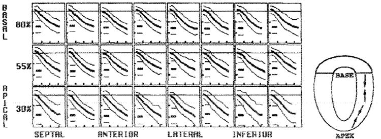
In each box, the evolution curves are shown as the mean (thick middle line) ± 2 SDs (thin outer lines). The short horizontal lines at the left in each box represent the mean and 2-SD peak values. The vertical ticks are spaced every 0.1. and the horizontal ticks are spaced every 100 msec. A schematic drawing of ELL is on the right. The ELL was homogeneous about the circumference and increased from base to the apex.
The three shear strains had a high degree of variability among the hearts, with wide SDs spanning the axis of zero strain. The average ERC was positive in all regions except the basal septum and had wide SDs spanning zero. There was no significant circumferential variation, but the ERC was lower at the basal level than it was at the equatorial (P = .04) or apical (P = .004) levels. The ERL also averaged near zero at the base and had wide SDs spanning zero throughout the LV. The ERL was lower anteriorly than it was at the other three sectors (P < .001) and was lower at the base than it was at the apex (P = .04). The ECL largely reflects the long-axis torsion of the LV. There was no significant circumferential variation, but the ECL was lower basally than it was equatorially (P = .04) or apically (P = .004). The mean ECL values (± SD) ranged from 0.01 ± 0.04 to 0.05 ± 0.05, corresponding to shear angles of approximately 1° to 5°.
The evolution of the average principal strains at the midwall is shown in Figure 8, and the average peak principal strains and angles are shown in Table 3. Any 3D strain tensor made up of axial and shear components can be expressed in a principal coordinate system, in which the shears along the axes become zero and the axial strain magnitudes are maximized. These three principal strains (eigen values of the strain tensor) are oriented along three mutually orthogonal directions that are called eigen vectors. In this study, the E1 (positive in sign) in the normal heart was approximately radially oriented, similar to the ERR. No significant spatial variation of the midwall first principal strain was found.
Figure 8. Average midwall principal strains.
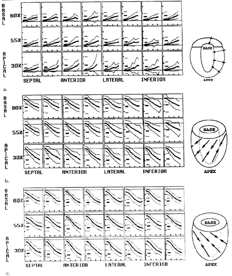
The (a) E1, (b) E2, and (c) E3 are illustrated. In each box, the evolution curves are shown as the mean (thick middle line) ± 2 SDs (thin outer lines). The short horizontal lines at the left in each box represent the mean and 2-SD peak values. The horizontal ticks are spaced every 100 msec, and the vertical ticks are spaced every 0.8 in a and every 0.1 in b and c. The drawings to the right of each array plot illustrate typical directions of strain.
TABLE 3.
Average Peak Principal Strains
| Strain | Septal | Anterior | Lateral | Inferior |
|---|---|---|---|---|
| E1 | ||||
| Basal | 0.46 ± 0.13 | 0.43 ± 0.22 | 0.53 ± 0.20 | 0.43 ± 0.17 |
| θRC | −1 ± 5 | 4 ± 5 | 4 ± 5 | 1 ± 9 |
| θRL | 3 ± 8 | −5 ± 6 | 4 ± 5 | 1 ± 10 |
| Equatorial | 0.45 ± 0.17 | 0.54 ± 0.26 | 0.40 ± 0.19 | 0.37 ± 0.22 |
| θRC | 2 ± 18 | 7 ± 5 | 5 ± 6 | 6 ± 8 |
| θRL | 8 ± 15 | 1 ± 6 | 8 ± 6 | 4 ± 9 |
| Apical | 0.42 ± 0.21 | 0.69 ± 0.31 | 0.51 ± 0.30 | 0.43 ± 0.40 |
| θRC | 11 ± 12 | 6 ± 6 | 4 ± 8 | 6 ± 9 |
| θRL | 7 ± 7 | 1 ± 6 | 5 ± 8 | 9 ± 14 |
| E2 | ||||
| Basal | −0.12 ± 0.03 | −0.14 ± 0.03 | −0.14 ± 0.03 | −0.11 ± 0.06 |
| θRC | 97 ± 21 | 77 ± 27 | 103 ± 15 | 92 ± 21 |
| θCL | 69 ± 30 | 73 ± 20 | 67 ± 12 | 46 ± 16 |
| Equatorial | −0.13 ± 0.03 | −0.15 ± 0.03 | −0.14 ± 0.04 | −0.12 ± 0.04 |
| θRC | 99 ± 13 | 101 ± 29 | 121 ± 25 | 101 ± 27 |
| θCL | 42 ± 31 | 72 ± 17 | 75 ± 18 | 50 ± 27 |
| Apical | −0.17 ± 0.04 | −0.17 ± 0.04 | −0.18 ± 0.03 | −0.18 ± 0.04 |
| θRC | 110 ± 23 | 98 ± 17 | 103 ± 38 | 113 ± 33 |
| θCL | 55 ± 35 | 65 ± 27 | 61 ± 19 | 64 ± 29 |
| E3 | ||||
| Basal | −0.20 ± 0.03 | −0.23 ± 0.03 | −0.23 ± 0.03 | −0.22 ± 0.03 |
| θRC | 88 ± 7 | 96 ± 6 | 92 ± 6 | 90 ± 15 |
| θCL | −21 ± 30 | −17 ± 21 | −23 ± 12 | −44 ±14 |
| Equatorial | −0.21 ± 0.03 | −0.26 ± 0.03 | −0.24 ± 0.02 | −0.22 ± 0.03 |
| θRC | 83 ± 11 | 97 ± 6 | 93 ± 7 | 93 ± 10 |
| θCL | −47 ± 31 | −18 ± 14 | −16 ± 16 | −40 ± 25 |
| Apical | −0.24 ± 0.03 | −0.28 ± 0.03 | −0.27 ± 0.03 | −0.26 ± 0.03 |
| θRC | 96 ± 19 | 95 ± 10 | 92 ± 6 | 91 ± 9 |
| θCL | −36 ± 31 | −25 ± 25 | −29 ± 18 | −26 ± 26 |
Note.—Data are the mean ± SD. Principal angles (θ) are in degrees. (See figure 2 for angle definitions). The first principal strain (E1), the strain of greatest elongation, was approximately radially oriented (θRC and θRL, ≈0°) and greater than zero, which indicated thickening. The SDs of the E1 were larger than those of the other principal strains. The middle principle strain (E2) and principal strain of greatest contraction (E3) both were approximately within the plane of the wail (θRC near 90°) and demonstrated contraction. The mean angle within the wall of the greatest contraction (E3θCL) ranged from −17° to −47°, approximating the expected orientation of the epicardial muscle fibers. Basal values were at 80% of the distance from the apex to the valve plane; equatorial values, at 55%; and apical values, at 30%.
The E3 (negative in sign) was oriented approximately within the circumferential-longitudinal plane and angled to spiral clockwise from the apex to the base, as viewed from the base (left-handed spiral). The E3 was greatest apically (P < .001 vs equatorially or basally) and greater in the anterior and lateral walls than in the septum (P < .001).
Finally, the E2 was approximately in the circumferential-longitudinal plane and greatest in magnitude apically (P < .001 vs equatorially or basally). The E2 was greater in maginitude at the lateral wall than it was at the inferior wall (P = .04).
Displacement and Rotation
The displacement evolution of the midwall material points from the end-diastolic geometry is platted in Figure 9. The average values of end-systolic displacement are shown in Table 4. There was significant spatial variation in displacement, even within individual sectors and levels. Radial displacement was directed inward (negative in sign) throughout the LV. The radial inward displacement was significantly smaller in the septum than in the lateral (P < .05) and inferior (P < .01) walls. It was greatest at the apical-inferior wall and least at the apical-anterior wall (P < .001)
Figure 9. Average midwall displacements.
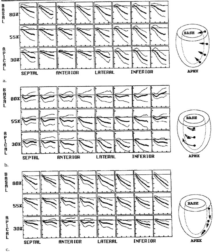
Average and 2-SD curves for (a) radial, (b) circumferential, and (c) longitudinal displacements (in mm) are shown. (a) Radial inward (negative) motion was heterogeneous and greatest in the anterior wall. (b) Average circumferential displacement (viewed front the base) was initially clockwise at the base before reversing and returning to nearly the starting position by end systole. At the apex, it was steadily clockwise, producing net torsion about the long axis by end systole. (c) The longitudinal motion in the base-to-apex direction (negative) was greatest at the base and least at the apex. In each panel, the horizontal ticks are spaced every 100 msec, and the vertical ticks are spaced every 4 mm. Typical motions are illustrated in the drawings on the right.
TABLE 4.
Average End-Systolic Displacement at the Middle Wall
| Displacement | Septal | Anterior | Lateral | Inferior |
|---|---|---|---|---|
| Radial | ||||
| Basal | −3.2 ± 2.0 | −5.8 ± 1.6 | −6.0 ± 1.9 | −4.9 ± 1.7 |
| Equatorial | −3.0 ± 2.3 | −3.7 ± 1.6 | −5.2 ± 1.6 | −5.2 ± 1.6 |
| Apical | −3.9 ± 1.8 | −2.4 ± 1.1 | −4.2 ± 1.3 | −6.3 ± 1.3 |
| Circumferential | ||||
| Basal | −1.8 ± 1.6 | −1.6 ± 1.8 | −1.4 ± 2.2 | −1.3 ± 2.4 |
| Equatorial | −2.4 ± 1.0 | −2.8 ± 2.0 | −3.9 ± 1.4 | −3.2 ± 1.9 |
| Apical | −1.9 ± 1.3 | −3.3 ± 1.9 | −5.5 ± 1.4 | −4.5 ± 1.8 |
| Longitudinal | ||||
| Basal | −8.1 ± 2.3 | −7.1 ± 1.9 | −8.8 ± 2.3 | −10.6 ± 1.9 |
| Equatorial | −5.7 ± 2.0 | −5.1 ± 2.0 | −6.7 ± 2.2 | −7.4 ± 1.6 |
| Apical | −3.5 ± 1.4 | −2.3 ± 1.7 | −4.9 ± 1.7 | −4.8 ± 1.4 |
Note.—Data are the mean ± SD, in millimeters. As shown in Figure 2, positive radial values were outward, positive circumferential values were in the plane of the heart wall directed counterclockwise as viewed from the base, and positive longitudinal values were in the plane of the heart wall direction, with an increase toward the base. Basal values were at 80% of the distance from the apex point to the valve plane; equatorial values, at 55% and apical values, at 30%.
Circumferential midwall displacement at the base, as viewed from the base, was clockwise (negative) about the long axis for the initial approximately 100 msec of systole, then it reversed to counterclockwise, with the basal material points ending up with little net change in circumferential position at end systole. Moving apically, the initial clockwise displacement increased and the final counterclockwise displacement decreased such that at the apical level, there was no final counterclockwise motion except at the septum. End-systolic circumferential displacement (magnitude) increased significantly from the basal to the equatorial levels (P < .001) and from the equatorial to the apical levels (P < .001). The circumferential displacement magnitude was greatest at the apical-lateral wall and was least at the inferior-basal wall (P < .001).
The rotation angle of material points about the long axis followed a pattern similar to that of circumferential displacement, except that it was homogeneous circumferentially due to the adjustment made for bulk heart translation.
Longitudinal motion was in the apical direction (negative in sign) throughout the LV, except for an initial transient basal displacement at the anterior apex. The end-systolic longitudinal displacement magnitude increased from the apical to the equatorial levels (P < .001) and from the equatorial to the basal levels (P < .001). Compared with that in the septal and lateral walls, the end-systolic longitudinal displacement magnitude was significantly greater in the inferior wall and significantly smaller in the anterior wall (P < .03 for each comparison).
The peak torsion angle, which is the peak change in the average rotation of a level with respect to the basal (80%) level, also was calculated. Positive values represent relative clockwise rotation of the more apical levels, as viewed from the base. The average peak torsion, in degrees and degrees per centimeter, at each level is illustrated in Figure 10. The torsion angle increased linearly toward the apex (r = −0.96; mean slope ± standard error of the mean, −0.255 ± 0.006, in degrees vs level in percentage). The torsion between adjacent levels, when normalized by using the mean separation between the levels at peak rotation, accounts for the decreasing separation between material point levels as the heart contracts. In our study, the normalized torsion increased nonlinearly toward the apex; this indicated an apical tightening of the rotational gradient along the long axis. This nonlinearity was also present in the subgroup of five hearts with data at all levels from 20%–80%.
Figure 10. Graphs illustrate the average peak torsion at midwall.
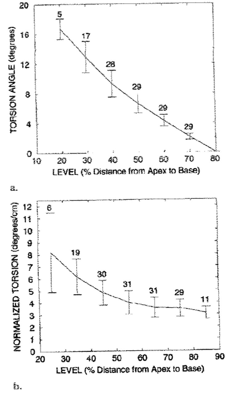
(a) The torsion angle was calculated relative to the most basal (80%) level and increased linearly toward the apex. The positive torsion angles represent the clockwise rotation of a level relative to the basal (80%) level, as viewed from the base. (b) The torsion between adjacent levels, as normalized by the long-axis separation at the deformed state, is shown. Normalized torsion increased nonlinearly toward the apex. In a and b, the mean value curve, SDs (vertical bars), and number of measurements at each level are shown.
Measurement Precision
Once the mean and SDs of the various strain components were determined, the measurement precision for each was estimated. The measurement precision of the given strain parameter is important because measurement uncertainty adds to the apparent normal range of strain (ie, the ± 2-SD line separation) among hearts. Due to differing amounts of tag data in different directions and the data averaging effects of composite parameters (wall thickening and SI), measurement precision was expected to vary among strain parameters. Precision was estimated on the basis of the smoothness of strain measurements among consecutive time frames, because the computed strain at each time frame was an independent measurement. This temporal variability was quantified for a given heart and material point by taking the root mean squared deviation of the sequential strain measures about a cubic fit of strain versus time (all time frames) and expressing it as a percentage of maximal value of the fitted curve. This variability measurement was averaged among all midwall material points and all hearts. The smoothest strain measurements were those for the wall thickening (2.7%), SI (2.8%), and E3 (2.8%), followed by those for the ECC (3.3%), ELL(4.0%), E2 (6.5%), ECL (11.0%), E1 (12.0%), ERR (13.0%), ERC (20.0%), and ERL (23.0%). These results indicated that the wall thickening, SI, E3, and ECC parameters had the greatest measurement precision relative to magnitude (≤3.3% of the maximum value), and that the axial strains with large radial components (ERR and E1) had the least precision (12%–13% of the maximum value). Of the shears, the ECL had the highest precision, reflecting the high spatial density of the data and the effect of LV torsion.
Transmural Strain Gradients
Transmural gradients of strain also were determined for the strain parameters, with the exclusion of the ERR and E1, which did not have sufficient spatial resolution in the radial direction. The evolution of the average endocardial (red) and epicardial (black) axial strains and strain indexes is shown in Figure 11. A single 2-SD curve is shown for each strain and index, and the short horizontal lines at the left in each box represent the average and 2-SD range of the peak values. All of the average peak axial strains and indexes were significantly greater in magnitude at the endocardium than they were at the epicardiurn in each region (P < .005 for each strain/position pair, with the exception of the ELL at the basal septum [P < .05]). These radial gradients were expected from the geometric considerations and tissue incompressibility, because concentric shells of myocardium have proportionally greater changes in dimension with decreasing radius. Significant transrmural gradients of the shears were not consistently observed throughout the LV. The torsion angle between the basal (80%) and apical (30%) levels increased from the epicardium (10.0° ± 1.6) to the midwall (12.3° ± 2.3) and also from the midwall to the endocardium (13.9° ± 3.2); both differences were significant (P < .005).
Figure 11. Transmural variation of average axial strains and indexes.
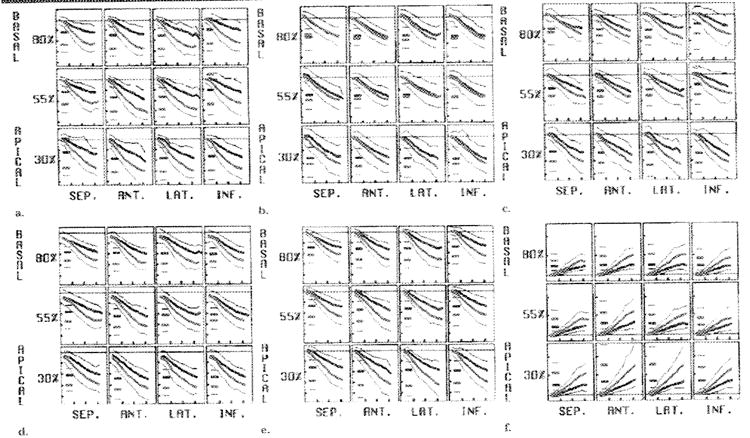
(a) ECC, (b) ELL, (c) E2, (d) E3, (e) SI, and (f) wall thickening are illustrated. As expected from geometric constraints, the mean axial strain magnitudes at the endocardium (thick red line) exceed those at the epicardium (thick black line); a single 2-SD curve (thin red and black lines) is shown for each. The short horizontal lines at the left in each box represent the mean and 2-SD values for the peak strain. The horizontal ticks are spaced every 100 msec, and the vertical ticks are spaced every 0,1 in a–e and every 0.8 in f. ANT. = anterior, INF. = inferior, LAT. = lateral, SEP. = septal.
The transmural parameters, when averaged spatially among the sectors and levels, are shown in Figure 12. With spatial averaging, significant radial gradients were also achieved with the shears (P < .001). All strain components and indexes increased from the epicardium to the endocardium, except for the ERL The spatially averaged E3θCL spiraled counterclockwise from the base to the apex and progressively less steeply from the epicardiurn (−43° ± 25) to the midwall (−29° ± 22) to the endocardium (−16° ± 19): both differences were significant (P < .005).
Figure 12. Graphs illustrate transmural variation of spatially averaged strains.
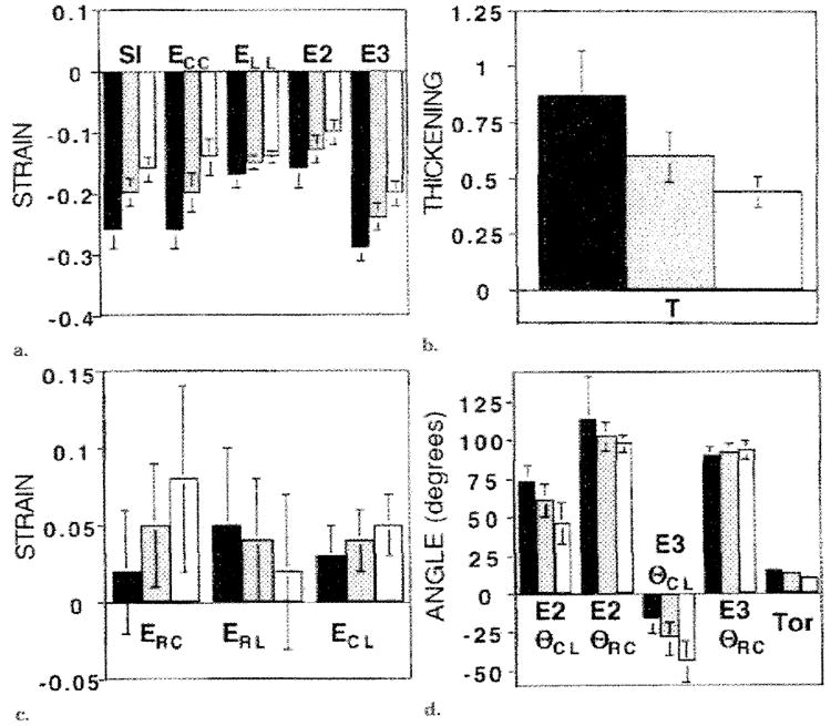
The black bars represent the values at the endocardium; gray bars, values at the midwall; and white bars, values at the epicardium. The (a) axial strains and SI, (b) wall thickening parameter, (c) shears, and (d) principal angles and the torsion angle between the 80% and 30% levels are illustrated. Significant transmural gradients were seen for all components (P < .005 for each). In b, T = wall thickening, and in d, Tor = torsion.
Example Use of Database
Finally, to illustrate the use of the strain database, the evolution of SI in a patient 3 months after a nontransmural inferior myocardial infarction is shown in Figure 13. The patient had no prior history of myocardial infarction and presented with chest pain and ST elevations in leads II, III, and aVF. The patient received thrombolytic agents, and the SI elevations normalized. The initial post-MI cardiac sonogram showed inferior hypokinesis with a qualitatively normal ejection fraction.
Figure 13. Use of the database of normal strain patterns to evaluate a postinfraction LV.
The SI evolution of a human LV 3 months after a nontransmural inferior infraction (thick line) is plotted with the two normal 2 SDs (thick lines) for each position. Relative to the normal range, there was a decrease in the strain rate (slope) and level of peak contraction in the inferior wall compared with that in the other regions. In addition, there was tranisent, early systolic wall stretching (intital positive values) in the basal inferior wall followed by contraction. The vertical ticks are spaced every 0.1, and the horizontal ticks are spaced everry 100 msec.
When the patient’s SI was plotted against the normal 2-SD lines for each midwall position, the location and degree of dysfunction were easily seen.
DISCUSSION
In this study, we described the normal systolic evolution of 3D strain throughout the human LV, with 32.5-msec temporal resolution, on the basis of cine MR imaging with tissue tagging. Prior to MR tagging and 3D reconstruction, it was not possible to acquire such detailed functional maps in the human hearts.
An important and potentially useful finding was that the normal ranges of strains, when plotted versus time, were small compared with the mean values, especially when strain parameters with high precision such as SI, wall thickening, E3, or ECC were used. Axial strains within the plane of the heart wall, especially the parameters derived from multiple such strains (ie, wall thickening and SI), are supported by the greatest amount of tag data due to the geometry of the heart; the circumference is much greater than the thickness, and there are many more tags around the circumference than across the wall (Fig 1). Because these parameters are well supported by the tag data in all directions, they are insensitive to noise on the tag data and can resolve gradients in the transmural direction.
In contrast, the strain parameters derived from radial displacements (ERR and E1) had the greatest variability over time and among hearts because they were based on the lowest spatial density of tag data (two to three across the wall). Thus for the detection of radial strain, the ERR cannot be measured as reproducibly as can the wall thickening parameter. In addition, the ERR was limited to nearly a constant value across the wall because the displacement function was limited to the first order in the radial direction due to the relative low tag spatial density. For these reasons, true radial strain was not well represented by using ERR measurements.
The wall thickening parameter was derived by using the incompressibility constraint. To the extent that the myocardium loses blood volume during systole, this parameter will overestimate true local wall, thickening. Cine radiographs of implanted beads (31) have shown volume losses of 0%–15%. Data in the canine LV from this laboratory (32) have shown average volume ratios of 0.94 ± 0.07, with normal perfusion and rations of 1.02 ± 0.06 during ischemia following occlusion of the left anterior descending coronary artery after the first diagonal branch. This change in volume ratio with ischemia was found to increase the sensitivity of the wall thickening parameter to that of ischemia. Thus, the wall thickening parameter reflects not only strains that contribute to thickening but also perfusion-related myocardial volume changes.
The SI parameter, which incorporates both the ECC and ELL, also is of particular interest because it has high precision owing to the large amount of supporting tag data, permits the detection of transmural strain gradients, and is insensitive to local variations of fiber angle due to its symmetry in the circumferential-longitudinal plane.
Although previously collected data on the evolution of local 3D strain in the human LV have been limited, the results from other studies generally are in good agreement with our results. With strain data based on implanted markers (5,6,27,33), and in previous studies with MR tagging (28,34-39), some normal human heart strains have been calculated. Ingels et al (5) implanted 12 arrays of tantalum screws in 15 transplanted hearts and found the peak shortening at the middle ventricular level (± SD) to range from 15% ± 4 to 19% ± 5 about the circumference compared with the 18% ± 3 to 26% ± 3 calculated in this study; in both studies, the maximum measurement was in the lateral wall. The longitudinal peak shortening observed by Ingels et al (5) ranged from 12% ± 5 to 13% ± 6 about the middle LV circumference at midwall compared with 16% ± 3 to 18% ± 3 in this study; both measurments were nearly spatially homogeneous. Their maximum peak shortening in the same region (15% ± 4 to 19% ± 5) was angled at a θCL of −45° ± 22.5, and orthogonal to this, the minimum was 11% ± 4 to 12% ± 5. These maximum and minimum strains correspond to our peak E3 (24% ± 4 to 30% ± 5) and E2 (11% ± 3 to 16% ± 3) values, respectively, when they are re-expressed as percent shortening. The implanted marker-based midwall strains in the study by Ingels et al were qualitatively similar but slightly lower in magnitude than those in this study. Limitations of the implantation method, such as changes from surgical transplantation, presence of metal helices in myocardium, and low spatial resolution, may account for these differences.
Clark et al (37) used MR imaging with tag grids on short-axis sections to calculate the circumferential component of end-systolic two-dimensional shortening in 10 normal LVs. Their average peak shortening for all segments in the LV at the endocardium, midwall, and epicardium were 44% ± 6, 30% ± 6, and 22% ± 5, respectively. These values were slightly higher than those in our study (32% ± 4, 23% ± 4, and 16% ± 4, respectively), but the measurements in both studies showed the average endocardial circumferential contraction to be double that at the epicardium and the ECC to increase from the base to the apex. The inability of the two-dimensional method to account for bulk motion of the heart through image sections and track the same tissue between the reference and deformed states, as well as differences in material point definition, may account for the minor differences. Kramer et al (35) and Palmon et al (34), both of whom used grid tagging in the short and long axes to evaluate the percentage of shortening circumferentially and longitudinally in 10 normal volunteers, produced data in close agreement to our values.
MacGowan et al (39) examined 10 healthy humans with MR tagging by using three radially oriented tag planes in the long axis and three parallel tag planes in the short axis to define 12 cuboids in the LV. Their average E3 at the epicardium. was −0.18 ± 0.03 at θCL of 75° ± 12, and that at the endocardium was −0.31 ± 0.03 at θCL of 6° ± 9. Although these E3θCL measurements were greater in magnitude than those in this study, both show a small change in E3θCL across the wall than would be expected from the transmural change in fiber orientation.
Young et al (38) used grid MR tagging and finite elements reconstruction to describe 3D end-systolic displacement and Lagrangian finite strain in 12 volunteers. All displacement and Lagrangian strain parameters were in close agreements with our data, with the exception that our midwall ERR values were greater (0.36–0.67 vs 0.02–0.25). These differences may be partially explained by the difficulty of the two MR tagging–based methods to generate more than, two lines across the heart wall, the relatively small amount of data in this direction, and the differences in 3D reconstruction technique. Our ERR values corresponded approximately to midwall thickening of 46%–80%. These data are in closer agreement with the other wall thickening estimates based on cine computed tomography (average, 66% ± 12 [40]; approximately 125% at the middle level [41]), short-axis cine MR imaging (56% ± 24 basally to 91% ± 29 apically [36]), and radially tagged MR imaging (55% ± 4 [39]). Lessiek et al (40) observed increasing base-to-apex gradients of thickening of approximately 50% ± 15 basally to 72% ± 18 apically; these values are in good agreement with those in our study.
Torsion of the LV also has been evaluated in transplanted human hearts with implanted markers. Hansen et al (27) found that torsion was altered even by subclinical bouts of rejection. They reported prerejection midwall torsion values of 5.7° ± 4 to 7.3° ± 5 at the middle ventricle and of 12.4° ± 6 to 15.3° ± 8 at the apex. On the basis of grid-tagged, two-dimensional MR imaging in healthy humans. Young et al (28) demonstrated a mean middle ventricular torsion of 4°–7° and a mean apical torsion of 12°–14°, with the endocardial torsion at the apex (16.5°) exceeding that at the epicardium (10.3°). By using two-dimensional spinecho MR imaging with radial tagging, Azhari et al (29) also reported that endocardial torsion (14.5°) exceeded epicardial torsion (9.2°) at the apex. Buchalter et al (30), by using the same imaging and tagging technique, reported a mean apical torsion of 12.2° ± 1.3 endocardially and of 11.2° ± 3 epicardially.
Although the detailed 3D displacement and strain evolution of the normal LV is complex, it can be summarized by using several overall principals and patterns. Displacement reflects the bulk translation and bulk rotation of the LV, as well as the local effects of strain; therefore, there is high spatial variation. For example, in our study, the apical level contained the inward radial displacement maximum (anteriorly) and minimum (inferiorly) due to bulk rotation of the LV about a transverse axis near the base. Strain, however, is independent of bulk motion, and in our study, it varied more predictably in the longitudinal and circumferential directions, tending to be greatest apically and in the free wall. During systole, the base descended toward the apex and the apex remained relatively fixed. There was also long-axis torsion produced by the domination of the epicardial muscle fibers, which spiral from the apex to the base in a clockwise direction, as viewed from the base. This torsion is reflected by the uniformly positive ECL, as well as by the negative E3θCL.
LV muscle fibers are angled approximately −60° to −80° from the circumferential direction at the epicardium, but they steadily rotate toward the circumferential direction at the midwall and to 60°–80° at the endocardium (39,42,43). This transmural variation of fiber angle results in variation of the E3θCL across the wall; tethering between layers of myocardium accounts for the much smaller gradient of E3θCL than fiber angle. The torsion serves to increase fiber contraction at the epicardium and decrease it at the endocardium. This tends to counter the opposite gradient caused by geometric constraints (ie, tissue incompressibility) and allows more equal muscle fiber contractions across the wall. With contraction, there is also rising cavity pressure, which tends to reshape the LV into a sphere (sphericalization), the shape of greatest volume. This rounding of the apex results in the nonlinear increase of normalized torsion toward the apex. Finally, normal axial strain magnitudes increase linearly with time for approximately the first half of systole before reaching a plateau and peaking at end systole.
The spatial heterogeneity of strain indicates that strain values should be compared with values that are normal for that region instead of with normal values for a remote zone, as has been done traditionally. This normal heterogeneity in individual hearts and the regional nature of ischemic dysfunction both support the need for this high-spatial-resolution strain database, with which the strain in individual hearts can be compared. Finally, the high temporal resolution of the described MR tagging method and of this database may permit the identification of abnormal strain transients or delays in contraction, even when peak strain attains a normal magnitude.
In conclusion, we used a noninvasive MR tagging and imaging technique to create a database of normal 3D systolic strain in the LV of healthy humans. In addition to evaluating conventional 3D strain components, displacements, and torsions, we identified composite parameters (SI and wall thickening) that had optimized precision, were supported by the greatest amount of tag data, and had the tightest normal variation among hearts. Spatial heterogeneity of strain was evaluated.
This normal 3D strain database is needed as a reference for evaluating the mechanical function of individual human hearts with MR tagging. Comparison of strain patterns in the human LV with those in this multidimensional database of normal strain patterns, with its high spatial and temporal resolution, may permit sensitive detection of mechanical dysfunction. Finally, the potential incorporation of this technique into a comprehensive cardiac examination with other MR modalities such as perfusion, angiography, and spectroscopy may greatly strengthen its potential for the noninvasive clinical evaluation of heart disease.
Abbreviations
- LV
left ventricle
- SI
shortening index
- 3D
three-dimensional
Appendix A
Harmonic Fitting Polynomial
Once a least-squares optimized fit to all the one-dimensional tag displacement data is made to a global 3D cartesian deformation gradient tensor, the residual tag point displacements are fit to spherical harmonics, with the exception that prolate spheroidal coordinates replace spherical coordinates as follows:
| (A1) |
where Term (i) is the i-th term of the polynomial expansion, N is the radial order of the fit (N = 1), λ is the prolate radial coordinate, L is the angular coordinate order (L = 4), a(i) is the unknown coefficient of the i-th term, P is the Legendre polynomial, ϕ is the prolate longitudinal angle coordinate, and θ is the circumferential angle coordinate. The residual displacement data from all tag points are simultaneously fit as a function position in prolate spheroidal coordinates to solve for the a(i) coefficients. The 3D displacement at any position in the LV can then be calculated by evaluating the polynomial expansion (21).
APPENDIX B
Derivation of the SI
The undeformed unit area in the circumferential-longitudinal plane is defined by the unit vectors C = (0,1,0) and L = (0,0,1). The deformed area is represented by these vectors after they are transformed to the deformed state by multiplication with the stretch tensor U. Thus, the deformed circumferential vector becomes
| (B1) |
Similarly, the deformed state of L is (URL, UCL, ULL). The area defined by the vectors in the deformed state is the magnitude of their cross product, which is expressed as follows: deformed area = ∣(URC, UCC, ULC) × (URL, UCL, ULL)∣. The ratio of the deformed area to the undeformed area is simply the deformed area because, by definition, the unit vectors C and L defined an area of 1.0. To derive the geometric mean of linear shortening, the square root of this area ratio is taken. Finally, for the SI to equal zero when there is no deformation (U = I and URR = 1.0), 1.0 is subtracted. This gives Equation (1):
| (1) |
APPENDIX C
Derivation of the Wall Thickening Parameter
The incompressibility constraint is met by setting the determinate of U to equal 1.0. The determinate of U is defined as follows:
| (C1) |
Next, the poorly measured URR component is replaced by (T + 1.0), with the 1.0 offset included such that T equals zero with no strain (URR = 1.0). Setting the Det(U) to equal 1.0 and substituting (T + 1.0) for URR gives the following equation:
Finally, solving for T gives Equation (2):
| (2) |
Footnotes
Supported in part by the National institutes of Health grants HL45090 and HL45683. C.C.M. supported in part by a fellowship from the Merck Sharp & Dohme Corporation. E.R.M. is an investigator with the American Heart Association.
References
- 1.Potel MJ, Rubin JM, MacKay SA, Aisen AM, AISadar J, Sayre RE. Methods for evaluating cardiac will motion in three dimensions using bifurcation points of the coronary artery tree. Invest Radiol. 1983;18:47–57. doi: 10.1097/00004424-198301000-00009. [DOI] [PubMed] [Google Scholar]
- 2.Young AA, Hunter PJ, Smaill BH. Estimation of epicardial strain using the motions of coronary bifurcations in biplane cineangiography. IEEE Trans Biomed Eng. 1992;39:526–531. doi: 10.1109/10.135547. [DOI] [PubMed] [Google Scholar]
- 3.Ingels NB, Daughters GT, Stinson EB, Alderman EL. Measurement of midwall myocardial dynamics in intact man by radiography of surgically implanted markers. Circulation. 1975;52:859–867. doi: 10.1161/01.cir.52.5.859. [DOI] [PubMed] [Google Scholar]
- 4.Hansen D, Daughters G, II, Alderman E, Ingels N, Jr, Miller DC. Torsional deformation of the left ventricular midwall in human hearts with intramyocardial markers: regional heterogeneity and sensitivity to the inotropic effects of abrupt rate changes. Circ Res. 1988;62:941–952. doi: 10.1161/01.res.62.5.941. [DOI] [PubMed] [Google Scholar]
- 5.Ingels NB, Jr, Hansen DE, Daughters GT, II, Stinson EB, Alderman EL, Miller DC. Relation between longitudinal, circumferential, and oblique shortening and torsional deformation in the left ventricle of the transplanted human heart. Circ Res. 1989;64:915–927. doi: 10.1161/01.res.64.5.915. [DOI] [PubMed] [Google Scholar]
- 6.Hansen DE, Daughters GT, II, Alderman EL, Ingels NB, Stinson EB, Miller DC. Effect of volume loading, pressure loading, and inotropic stimulation on left ventricular torsion in humans. Circulation. 1991;83:1315–1326. doi: 10.1161/01.cir.83.4.1315. [DOI] [PubMed] [Google Scholar]
- 7.Yun KL, Niczyporuk MA, Daughters GT, II, et al. Alterations in left ventricular diastolic twist mechanics during acute human cardiac allograft rejection. Circulation. 1991;83:962–973. doi: 10.1161/01.cir.83.3.962. [DOI] [PubMed] [Google Scholar]
- 8.Zerhouni EA, Parish DM, Rogers WJ, Yang A, Shapiro EP. Human heart: tagging with MR imaging—a method for noninvasive assessment of myocardial motion. Radiology. 1988;169:59–63. doi: 10.1148/radiology.169.1.3420283. [DOI] [PubMed] [Google Scholar]
- 9.Axel L, Dougherty L. MR imaging of motion with spatial modulation of magnetization. Radiology. 1989;171:841–849. doi: 10.1148/radiology.171.3.2717762. [DOI] [PubMed] [Google Scholar]
- 10.Axel L, Dougherty L. Heart wall motion: improved method of spatial modulation of magnetization for MR imaging. Radiology. 1989;172:349–350. doi: 10.1148/radiology.172.2.2748813. [DOI] [PubMed] [Google Scholar]
- 11.Mosher TJ, Smith MB. A DANTE tagging sequence for the evaluation of translational sample motion. Magn Reson Med. 1990;15:334–339. doi: 10.1002/mrm.1910150215. [DOI] [PubMed] [Google Scholar]
- 12.Bolster BD, McVeigh ER, Zerhouni EA. Myocardial tagging in polar coordinates with striped tags. Radiology. 1990;177:769–772. doi: 10.1148/radiology.177.3.2243987. [DOI] [PMC free article] [PubMed] [Google Scholar]
- 13.McVeigh ER, Zerhouni EA. Noninvasive measurement of transmural gradients in myocardial strain with MR imaging. Radiology. 1991;180:677–683. doi: 10.1148/radiology.180.3.1871278. [DOI] [PMC free article] [PubMed] [Google Scholar]
- 14.McVeigh ER, Atalar E. Cardiac tagging with breath hold CINE MRI. Magn Reson Med. 1992;28:318–327. doi: 10.1002/mrm.1910280214. [DOI] [PMC free article] [PubMed] [Google Scholar]
- 15.Pipe JG, Boes JL, Chenevert TL. Method for measuring three-dimensional motion with tagged MR imaging. Radiology. 1991;181:591–595. doi: 10.1148/radiology.181.2.1924810. [DOI] [PubMed] [Google Scholar]
- 16.Young AA, Axel L, Dougherty L, Parenteau CS. Validation of tagging with MR imaging to estimate material deformation. Radiology. 1993;188:101–108. doi: 10.1148/radiology.188.1.8511281. [DOI] [PubMed] [Google Scholar]
- 17.Lima JA, Jeremy R, Guier W, et al. Accurate systolic wall thickening by nuclear magnetic resonance imaging with tissue tagging: correlation with sonomicrometers in normal and ischemic myocardium. J Am Coll Cardiol. 1993;21:1741–1751. doi: 10.1016/0735-1097(93)90397-j. [DOI] [PubMed] [Google Scholar]
- 18.Moore CC, Reeder SB, McVeigh ER. Tagged MR imaging in a deforming phantom: Photographic validation. Radiology. 1994;190:765–769. doi: 10.1148/radiology.190.3.8115625. [DOI] [PMC free article] [PubMed] [Google Scholar]
- 19.Moore CC, O’Dell WG, McVeigh ER, Zerhouni EA. Calculation of three-dimensional left ventricular strains from biplanar tagged MR images. J Magn Reson Imaging. 1992;2:156–175. doi: 10.1002/jmri.1880020209. [DOI] [PMC free article] [PubMed] [Google Scholar]
- 20.Young AA, Axel L. Three-dimensional motion and deformation of the heart wall: estimation with spatial modulation of magnetization—a model-based approach. Radiology. 1992;185:241–247. doi: 10.1148/radiology.185.1.1523316. [DOI] [PubMed] [Google Scholar]
- 21.O’Dell WG, Moore CC, Hunter WC, Zerhouni EA, McVeigh ER. Three-dimensional myocardial deformations: calculation with displacement field fitting to tagged MR images. Radiology. 1995;195:829–835. doi: 10.1148/radiology.195.3.7754016. [DOI] [PMC free article] [PubMed] [Google Scholar]
- 22.Denney TS, McVeigh ER. Model-free reconstruction of three-dimensional myocardial strain from planar tagged MR images. J Magn Reson Imaging. 1997;7:799–810. doi: 10.1002/jmri.1880070506. [DOI] [PMC free article] [PubMed] [Google Scholar]
- 23.McVeigh ER. MRI of myocardial function: motion tracking techniques. Magn Reson Imaging. 1996;14:137–150. doi: 10.1016/0730-725x(95)02009-i. [DOI] [PubMed] [Google Scholar]
- 24.Croisille P, Guttman MA, Atalar E, McVeigh ER, Zerhouni EA. Precision of myocardial contour estimation from tagged ME images with a “black-blood” technique. Acad Radiol. 1998;5:93–100. doi: 10.1016/s1076-6332(98)80128-1. [DOI] [PMC free article] [PubMed] [Google Scholar]
- 25.Guttman MA, Zerhouni EA, McVeigh EM. Analysis and visualization of cardiac function from MR images. IEEE Comput Graph Appl. 1997;17:30–38. doi: 10.1109/38.576854. [DOI] [PMC free article] [PubMed] [Google Scholar]
- 26.Bazille A, Guttman MA, McVeigh ER, Zerhouni EA. Impact of semi-automated versus manual image segmentation errors on myocardial strain calculation by MR tagging. Invest Radiol. 1994;294:427–433. doi: 10.1097/00004424-199404000-00008. [DOI] [PMC free article] [PubMed] [Google Scholar]
- 27.Hansen DE, Daughters GT, II, Alderman EL, Stinson EB, Baldwin JC, Miller DC. Effect of acute human cardiac allograft rejection on left ventricular systolic torsion and diastolic recoil measured by intramyocardial markers. Circulation. 1987;76:998–1008. doi: 10.1161/01.cir.76.5.998. [DOI] [PubMed] [Google Scholar]
- 28.Young AA, Imai H, Chang CN, Axel L. Two-dimensional left ventricular deformation during systole using magnetic resonance imaging with spatial modulation of magnetization. Circulation. 1994;89:740–752. doi: 10.1161/01.cir.89.2.740. [DOI] [PubMed] [Google Scholar]
- 29.Azhari H, Buchalter M, Sideman S, Shapiro E, Beyar R. A conical model to describe the nonuniformity of left ventricular twisting motion. Ann Biomed Eng. 1992;20:149–165. doi: 10.1007/BF02368517. [DOI] [PubMed] [Google Scholar]
- 30.Buchalter MB, Weiss JL, Rogers WJ, et al. Noninvasive quantification of left ventricular rotational deformation in normal humans using magnetic resonance imaging myocardial tagging. Circulation. 1990;81:1236–1244. doi: 10.1161/01.cir.81.4.1236. [DOI] [PubMed] [Google Scholar]
- 31.Waldman LK, Fung YC, Covell JW. Transmural myocardial deformation in the canine left ventricle. Circ Res. 1985;57:152–163. doi: 10.1161/01.res.57.1.152. [DOI] [PubMed] [Google Scholar]
- 32.Moore CC, McVeigh ER, Zerhouni EA. Non-invasive measurement of three dimensional myocardial deformation with MRI tagging during graded local ischemia. J Cardiovasc Magn Med. 1999;1(3):207–222. doi: 10.3109/10976649909088333. [DOI] [PMC free article] [PubMed] [Google Scholar]
- 33.Moon MR, Ingels NB, Jr, Daughters GT, II, Stinson EB, Hansen DE, Miller DC. Alterations in left ventricular twist mechanics with inotropic stimulation and volume loading in human subjects. Circulation. 1994;89:142–150. doi: 10.1161/01.cir.89.1.142. [DOI] [PubMed] [Google Scholar]
- 34.Palmon LC, Reichek N, Yeon SB, et al. Intramural myocardial shortening in hypertensive left ventricular hypertrophy with normal pump function. Circulation. 1994;89:122–131. doi: 10.1161/01.cir.89.1.122. [DOI] [PubMed] [Google Scholar]
- 35.Kramer CM, Reichek N, Ferrari VA, Theobald T, Dawson J, Axel L. Regional heterogeneity of function in hypertrophic cardiomyopathy. Circulation. 1994;90:186–194. doi: 10.1161/01.cir.90.1.186. [DOI] [PubMed] [Google Scholar]
- 36.van Rugge FP, Holman ER, van der Wall EE, de Roos A, van der Laarse A, Bruschke AV. Quantification of global and regional left ventricular function by cine magnetic resonance imaging during dobutamine stress in normal human subjects. Eur Heart J. 1993;14:456–463. doi: 10.1093/eurheartj/14.4.456. [DOI] [PubMed] [Google Scholar]
- 37.Clark NR, Reichek N, Bergey P, et al. Circumferential myocardial shortening in the normal human heart: assessment by magnetic resonance imaging using spatial modulation of magnetization. Circulation. 1991;84:67–74. doi: 10.1161/01.cir.84.1.67. [DOI] [PubMed] [Google Scholar]
- 38.Young AA, Kramer CM, Ferrari VA, Axel L, Reichek N. Three-dimensional left ventricular deformation in hypertrophic cardiomyopathy. Circulation. 1994;90:854–867. doi: 10.1161/01.cir.90.2.854. [DOI] [PubMed] [Google Scholar]
- 39.MacGowan GA, Shapiro EP, Azhari H, et al. Noninvasive measurement of shortening in the fiber and cross-fiber directions in the normal human left ventricle in idiopathic dilated cardiomyopathy. Circulation. 1997;96:535–541. doi: 10.1161/01.cir.96.2.535. [DOI] [PubMed] [Google Scholar]
- 40.Lessick J, Fisher Y, Beyar R, Sideman S, Marcus ML, Azhari H. Regional three-dimensional geometry of the normal human left ventricle using cine computed tomography. Ann Biomed Eng. 1996;24:583–594. doi: 10.1007/BF02684227. [DOI] [PubMed] [Google Scholar]
- 41.Taratorin AM, Sideman S. 3D functional mapping of left ventricular dynamics. Comput Med Imaging Graph. 1995;19:113–129. doi: 10.1016/0895-6111(94)00038-7. [DOI] [PubMed] [Google Scholar]
- 42.Streeter DD. Gross morphology and fiber geometry of the heart. In: Berne RM, editor. Handbook of physiology. Section 2. The cardiovascular system. Vol. 1. Washington, DC: American Physiological Society; 1979. pp. 61–112. [Google Scholar]
- 43.Nielsen PM, Le Grice IJ, Smaill BH, Hunter PJ. Mathematical model of geometry and fibrous structure of the heart. Am J Physiol. 1991;260:H1365–1378. doi: 10.1152/ajpheart.1991.260.4.H1365. [DOI] [PubMed] [Google Scholar]