Pencil Excitation with Interleaved Fourier Velocity Encoding: NMR Measurement of Aortic Distensibility

Abstract

A technique is presented for rapidly and noninvasively determining aortic distensibility, by NMR measurement of pulse-wave velocity in the aorta. A cylinder of magnetization is excited along the aorta, with Fourier-velocity encoding and readout gradients applied along the cylinder axis. Cardiac gating and data interleaving improve the effective time resolution to as high as 3 ms. Wave velocities are determined from the position of the foot of the flow wave in the velocity profiles. Evidence of helical flow distal to the aortic arch can be seen in normal subjects, while disturbed flow patterns are visible in patients with aneurysms and dissections.

INTRODUCTION

Aortic stiffness appears to be a correlate of age, fitness, and coronary artery disease (1-3). It has been shown to influence left ventricular afterload and is an important variable in the management of ventricular disease (4-6). A drop in aortic distensibility may contribute to increased left ventricular mass in postmenopausal women. Also, in patients with aneurysmal dilation secondary to atherosclerosis or connective tissue disease, aneurysmal distensibility and diameter may be better indicators of the risk of sudden aortic dissection or rupture than diameter alone. A rapid and noninvasive technique for determining aortic distensibility could prove an important tool in all of these contexts.

A number of techniques have been proposed for the determination of aortic stiffness, some based on the measurement of variations in aortic diameter and blood pressure over the cardiac cycle (2, 3, 7), and others measuring the velocity of propagation of the pressure or flow wave along the aorta (8-13). Those in the former category are limited by the need to measure local blood pressure, and estimates based on peripheral blood pressure typically are used. Of the latter class, most either employ Doppler ultrasound (12, 13) or NMR (9-11) determinations of velocity, to time the passage of the flow wave. Many of these techniques are limited as to the region in which measurements can be made, and typically two specific points, e.g., the aortic arch and a spot on the femoral artery (13) are chosen.

One recent technique (9) uses NMR excitation of a cylinder or “pencil” aligned with the aorta to produce M-mode phase-contrast aortic blood-flow images, with cardiac gating and data interleaving employed to increase the effective time resolution. This technique has been applied to measure wave velocity in patients with Marfan syndrome and other connective tissue diseases (14). For some patients with weak blood flow or irregular heartbeat, however, this method can produce large measurement uncertainties.

We present here a similar but more robust cardiacgated NMR technique for determining aortic distensibility (15). An NMR pencil-excitation pulse is again used, with a bipolar velocity-encoding gradient and then a readout gradient applied along the pencil axis, and with data interleaving employed to improve the effective time resolution so that rapid propagation of wavefronts can be followed. In this method, however, the bipolar gradient is stepped through a range of values, with a Fourier transform applied to produce velocity distribution profiles for different phases of the heart cycle (16, 17). If a sinusoidal bipolar gradient is employed which has maximum amplitude G and separation between lobe centers of T, then the velocity resolution V_res obtained with this method is

$$V_{\mathit{res}}=\frac{{\pi }^2}{2\gamma {\mathit{GT}}^2},$$ [1]

where γ is the gyromagnetic ratio. The resulting velocity distributions can be played as a video loop, in which the velocity wave can be seen propagating along the aorta. The position of the foot of the wave can be measured at successive heart phases and used to determine the wave velocity. An added benefit of this technique is that it provides details of normal and abnormal flow patterns in the aorta, as well as quantitative velocity information.

The wave speed C and the density ρ of the blood in the vessel can be used to determine the vessel distensibility D, according to the relation

$$D=1∕\rho C^2,$$ [2]

where the distensibility is defined as the fractional change in vessel cross-sectional area per unit change in pressure (18, 19). For an incompressible fluid in a stiff vessel, pressure changes are instantaneously transmitted down the vessel, but for a vessel with compliant walls, the pressure wave distends the vessel, and travels along it at a finite velocity.

MATERIALS AND METHODS

The GE Signa MRI scanner was controlled interactively (9, 20) from a Sun SPARCstation using a specially designed interface developed at GE Medical Systems. This uses a Bit3 bus adapter as a data path and an Ethernet connection as a scan-control path. New pencil orientations and offsets were prescribed graphically on a scout image displayed on the Sun, and sent over the scan-control link to interactively redirect the pulse sequence. Either a phased-array surface coil set or a body-coil receiver was used to obtain scout and velocity images.

The basic cardiac-gated 1D Fourier velocity-encoded pulse sequence (16) is shown in Fig. 1. This sequence was gated to the cardiac R-wave and executed 16 times per heart cycle. The bipolar gradient was stepped to a new value on each new trigger and a 2D Fourier transform applied to produce blood velocity profiles every 24–36 ms over the cardiac cycle. To improve the effective time resolution, the cardiac trigger delay was incremented 4 to 8 times, with the increment chosen to yield equal time intervals between phases, as illustrated in Fig. 2. The acquired data were then interleaved into the proper time order. The resulting time series of velocity distribution profiles had distance along the excited pencil as one axis, and velocity as the other axis. The sequence typically employed 16 velocity-encoding steps, with a bipolar-gradient maximum amplitude of 1 G/cm, and a duration for each lobe of 4.3 ms, yielding a velocity resolution of 10 cm/s, which was judged sufficient for accurate tracking of the foot of the flow wave. This set of parameters resulted in aliasing for velocities greater than 80 cm/s (our “Nyquist velocity”), but because the flow direction was known, and flow was followed over the heart cycle, any ambiguity in the velocity distributions was removed, and higher velocities could be unwrapped. Alternatively, a velocity resolution of 5 cm/s was obtained, with the same peak velocity, when the bipolar gradients were stepped through 32 levels with a peak amplitude of 1 G/cm and a width of 6 ms for each gradient lobe. In this manner, an effective time resolution of 3–7 ms and a velocity resolution of 5–10 cm/s were achieved in a 1- to 4-min examination.

FIG. 1.

Basic cardiac-gated velocity-profiling pulse sequence. Spiral-scan pulse excites a pencil of magnetization, and a bipolar flow-encoding pulse and half-echo readout are applied along the pencil axis. The amplitude of the bipolar waveform is stepped on each heartbeat, and 2DFTs applied to the raw signals, to yield a time series of velocity-distribution profiles along the pencil.

FIG. 2.

Cardiac gating scheme for interleaved velocity-profiling sequence. Sixteen phases of the heart are acquired in each heartbeat, with the trigger delay incremented, e.g., on 4 successive heartbeats, and the velocity-encoding gradients stepped, e.g., through 16 groups of heartbeats. The data are then interleaved into the proper time order and a 2DFT applied to each frame.

The field of view was typically 24–32 cm and the pencil diameter, 1.5–3 cm. The pencil-excitation pulse was based on an 8-cycle k-space spiral (21), and ranged from 9–13 ms in duration. The RF waveform was compensated for nonuniform sampling of k-space by the spiral near its center, to improve the sharpness of the excitation profile (22). The spiral was traversed at a nonuniform angular rate, to yield a constant gradient slew rate and thus shorter duration and higher excitation bandwidth (23). Still higher bandwidth and fewer off-resonance problems can be achieved by using spirals of fewer cycles, interleaving or pinwheeling the spirals, and adding the resulting signals (24). A 6-ms-long 4-cycle spiral was in some cases employed, in place of the 8-cycle spiral. This was pinwheeled through two interleaves to double the radius of the innermost sampling ring artifact (24), thus pushing it outside of the body for most applications. In practice the double-spiral pinwheeling was achieved by inverting all of the 2D-excitation pulse waveforms on alternate excitations, and subtracting the acquired signals. These included the two gradient waveforms, the RF waveform, and the phase waveform used to offset the pencil from gradient isocenter. This doubled the number of excitations and thus the total data acquisition time.

RESULTS

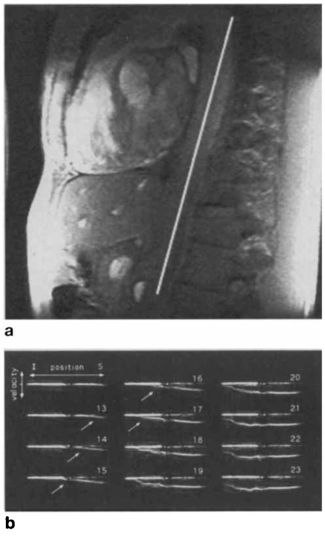
Figure 3a shows a scout image of the descending aorta of a normal volunteer, acquired with the phased array, with the line on the image denoting pencil position for the subsequent 1D velocity sequence. The pulse sequence of Fig. 1 was then applied, with the excited pencil and the flow-encoding direction running along the aorta. Here the pencil diameter was 1.5 cm, TR was 36 ms, and 32 velocity-encoding steps were applied. The resulting velocity distribution, shown over 12 of 16 heart phases, is illustrated in Fig. 3b. The long horizontal line in each frame corresponds to static tissue in the excited pencil, at each cardiac phase. Vertical displacements relative to each long line are proportional to velocity at that heart phase. Note that in this and all other data sets, the superior direction is taken to be positive, so that the right side of each trace corresponds to the superior end of the pencil, and blood moving in an inferior direction is taken to have negative velocities, i.e., negative displacements relative to the zero-velocity line. Where the pencil falls inside the aorta, a segment can be seen in Fig. 3b rising and then falling over the cardiac cycle, resulting from pulsatile blood flow in the aorta. The peak velocity for this volunteer was 115 cm/s. It can be seen in Phases 3–5 that the flow wave reaches the superior portion of this section of the aorta (see Fig. 3a) first, and then rapidly propagates down the aorta at a rate too fast to quantify accurately with this noninterleaved version of the pulse sequence. A disturbance can be seen in the flow near peak systole, starting at the superior end of the flow profile in Phase 7 and propagating distally through Phases 8–10 (arrows). The velocity of propagation of the disturbance, measured to be 89 ± 5 cm/s initially and decreasing to 29 ± 5 cm/s as the disturbance moves distally, is much slower than the propagation velocity of the flow wave itself.

FIG. 3.

(a) Oblique coronal scout image of descending aorta of a normal volunteer. Line indicates position of prescribed 1.5-cm diameter pencil for Fourier velocity sequence. (b) Results of Fourier velocity-encoded pulse sequence of Fig. 1, over 12 of 16 heart phases. Horizontal displacement is position along the pencil and vertical displacement is blood velocity, which reaches a peak value of 115 cm/s in frame No. 6. Arrows denote propagating disturbance assigned to helical flow patterns. FOV was 24 cm. I = inferior, S = superior.

Figure 4a shows a scout image from a normal volunteer of age 38 years, acquired with the phased array, with the line again indicating the position of the excited pencil in the subsequent 1D velocity image. In this case, an interleaved version of the pulse sequence was applied, as in Figs. 1 and 2, with a pencil diameter of 3 cm, 16 velocity-encoding steps, 4 interleaves, and a TR of 28.8 ms. This produced velocity profiles over 64 phases of the heart cycle, with an effective time resolution of 7.2 ms. Phases 12–23 are shown in Fig. 4b. The velocity wave can be seen rising at the superior end of the vessel and propagating down the aorta. In each frame the position of the foot of the wave, defined as the point at which it rises from zero velocity, was determined by template matching to an accuracy of approximately ±4 mm. Linear regression on the position of the foot of the wave versus time for Frames 13–17 yielded a propagation velocity of 508 ± 16 cm/s, where the uncertainty is the variance determined from the χ² fit. For comparison's sake, the phase-contrast analog of this pulse sequence (9) was also applied, producing a measured value of 550 ± 50 cm/s.

FIG. 4.

(a) Oblique sagittal scout image of descending aorta of a normal volunteer. Line indicates position of prescribed 3-cm diameter pencil for subsequent velocity sequence. (b) Interleaved velocity-distribution profiles obtained using the gating scheme of Fig. 2. Effective time resolution has been improved to 7.2 ms. Propagating wavefront can be seen in frames Nos. 12–18. FOV was 24 cm. I = inferior, S = superior.

The noninterleaved pulse sequence of Fig. 1 has been applied to a number of patients with aortic aneurysms and/or dissections secondary to Marfan syndrome or atherosclerosis. The following data were all acquired with a pencil diameter of 1.5 cm, a repetition time of 36 ms, 32 velocity-encoding steps, and a velocity range of ±80 cm/s. The solid lines on the left sides of Figs. 5a and 5b show the pencil prescription along the descending aorta of the same Marfan patient on two different occasions separated by 6 months. The right sides of the figures show portions of the corresponding velocity series. It can be seen that the profiles are dissimilar to those of the normal subjects, and also very reproducible. Figure 5c shows part of a velocity series taken through the aortic valve and ascending aorta of the same subject (dashed line on left side of Fig. 5a). It is evident from the prescription that the pencil also intersects a portion of the descending aorta. Note that distal flow produces positive velocities in the ascending aorta and negative velocities in the descending aorta in these data sets. Retrograde flow through the valve is seen as the negative velocities (arrow) in Frame 11. Figure 6 shows a velocity series from the descending aorta of another Marfan patient with an aortic dissection, showing nonuniform flow in the region of the dissection.

FIG. 5.

Scout image with position of 1.5-cm diameter pencil indicated as solid line (left), and corresponding velocity-distribution profiles (right) obtained from descending aorta of a Marfan patient initially (a) and 6 months later (b). Profiles look very similar. (c) Velocity profiles through the aortic valve of the same patient, using the pencil position denoted by the dashed line on the left side of (a). Aortic Insufficiency is Seen as retrograde flow in frame No. 11 (arrow). FOV was 32 cm. I = inferior, S = superior.

FIG. 6.

(a) Oblique sagittal scout image from a patient with an aortic dissection secondary to Marfan syndrome. Line indicates position of prescribed 1.5-cm diameter pencil for velocity sequence. (b) Velocity distribution profiles in the region of the dissection show nonuniform flow patterns. FOV was 30 cm. I = inferior, S = superior.

DISCUSSION

We have developed a noninvasive technique for accurately measuring aortic distensibility within a total of 64–256 heartbeats. NMR pencil excitation and Fourier velocity encoding are used to determine blood velocity to an accuracy of 5–10 cm/s, with a spatial resolution of about 1 mm and a time resolution of 24–36 ms. The effective time resolution of the technique is increased four- to eight-fold by using an interleaved version of the pulse sequence. The sequence is directed in a highly interactive fashion via a workstation interface to the MR scanner. This gives the ability to acquire regional measurements in a quick, noninvasive manner, over any portion of the aorta, along lengths as short as approximately 4–5 cm. It is sensitive over a range of distensibilities from approximately 10⁻⁶ to 10⁻³ m s²/kg, where the lower limit is determined by the time resolution of the technique, and the upper limit is reached as wave velocities approach the blood velocity. The wave velocity of 508 cm/s measured for the data set of Fig. 4b corresponds to an aortic distensibility of 37 pm s²/kg, a value consistent with measurements from other normal subjects of similar age (9).

An advantage of this technique is its intuitive appeal. The propagating wavefront is especially well visualized when the velocity frames are played in a movie loop.¹ Details of normal and abnormal velocity distributions in the aorta are readily seen with this method. For example, the flow disturbance shown in Fig. 3 (arrows) propagating down the descending aorta from the aortic arch is often visible in data sets from normal subjects, and appears to arise from helical flow patterns that develop below the arch after peak systole. Abnormal flow patterns in patients with Marfan syndrome are clearly visualized, and appear to be reproducible. The smearing of the velocity distribution at the superior end of the profiles in Figs. 5a and 5b, just below the aortic arch, is evident as a swirling pattern when the frames are played as a video loop. This effect is observed in the same patient on two different occasions 6 months apart, but does not appear to the same extent in any other subject examined so far. Retrograde flow through an incompetent aortic valve, as shown in Fig. 5d, is easily characterized with this technique, and appears to be accompanied in many patients by a spreading or blurring of the velocity distribution at the level of the valve during diastole. The velocity profile along the aortic dissection of Fig. 6 is characterized mainly by its nonuniform appearance.

This method is fairly robust relative to our previous phase-contrast pulse sequence (9). For instance, if the excited pencil is slightly misaligned with the aorta or has a larger diameter than the aorta, then partial voluming can occur from stationary tissue around the vessel. Static-field inhomogeneity and magnetic susceptibility effects can also cause a spreading of the pencil excitation region (21), increasing this partial-voluming effect. However, the Fourier velocity technique is relatively unaffected by this, because Fourier encoding pushes the signal from static tissue to a different part of the velocity spectrum from the signal from moving blood. In phase-contrast techniques, this signal from stationary tissue is averaged with the blood signal. In fact, the velocity distribution from the blood itself appears to comprise a single velocity in most cases, at least on the rising edge of the flow wave, corresponding to near-plug flow in the aorta. This produces a relatively sharp velocity trace, on which the foot of the flow wave is easily visualized.

We found our determination of wave velocity to be adversely affected in some cases by breathing artifacts, which took the form of signal dropout and/or ghosting in the velocity-encoding dimension, notably in that portion of the descending aorta at the level of the diaphragm. For instance, a slight disruption in the signal is seen at the center of the velocity profiles for the interleaved Fourier technique of Fig. 4b. Breath-holding has been found to ameliorate this problem considerably, but may not be practical for all patients. The use of repeated short breath-holds would prove beneficial in these cases; data acquisition could be triggered by real-time scout views, which monitored the start of breath-holding.

The interleaved version of this pulse sequence is relatively new and has not yet been used to determine pulse wave velocity in patients. We foresee no barriers, however, to the application of interleaving in a clinical setting. This technique should prove a fast and reliable method for determining aortic distensibility in a variety of disease states.

REFERENCES

- 1.Caro CG, Lever MJ, Parker KH, Fish PJ. Effect of cigarette smoking on the pattern of arterial blood flow: possible insight into mechanisms underlying the development of arteriosclerosis. Lancet. 1987 July;4:11–13. doi: 10.1016/s0140-6736(87)93052-2. [DOI] [PubMed] [Google Scholar]
- 2.Mohiaddin RH, Underwood SR, Bogren HG, Firmin DN, Klipstein RH, Rees RSO, Longmore DB. Regional aortic compliance studied by magnetic resonance imaging: the effects of age, training, and coronary artery disease. Br. Heart J. 1989;62:90–96. doi: 10.1136/hrt.62.2.90. [DOI] [PMC free article] [PubMed] [Google Scholar]
- 3.Dart AM, Lacombe F, Yeoh JK, Cameron JD, Jennings GL, Laufer E, Esmore DS. Aortic distensibility in patients with isolated hypercholesterolaemia, coronary artery disease, or cardiac transplant. Lancet. 1991;338:270–273. doi: 10.1016/0140-6736(91)90415-l. [DOI] [PubMed] [Google Scholar]
- 4.Wilcken DE, Charlier AA, Hoffmann JI, Guz A. Effects of alterations in aortic impedance on the performance of the ventricles. Circ. Res. 1964;14:283–293. doi: 10.1161/01.res.14.4.283. [DOI] [PubMed] [Google Scholar]
- 5.Urschel CW, Covel JW, Sonnenblick EH, Ross J, Braunwald E. Effects of decreased aortic compliance on performance of the left ventricle. Am. J. Physiol. 1968;214:298–304. doi: 10.1152/ajplegacy.1968.214.2.298. [DOI] [PubMed] [Google Scholar]
- 6.Firmin DN, Mohiaddin RH, Underwood SR, Longmore DB. Magnetic resonance imaging: a method for the assessment of changes in vascular structure and function. J. Hum. Hypertens. 1991;5:31–40. [PubMed] [Google Scholar]
- 7.Buonocore MH, Bogren H. Optimized pulse sequences for magnetic resonance measurement of aortic cross sectional areas. Magn. Reson. Imaging. 1991;9:435–447. doi: 10.1016/0730-725x(91)90433-m. [DOI] [PubMed] [Google Scholar]
- 8.Ting CT, Chang MS, Wang SP, Chiang BN, Yin FCP. Regional pulse wave velocities in hypertensive and normotensive humans. Cardiovasc. Res. 1990;24:865–872. doi: 10.1093/cvr/24.11.865. [DOI] [PubMed] [Google Scholar]
- 9.Hardy CJ, Bolster BD, McVeigh ER, Adams WJ, Zerhouni EA. A one-dimensional velocity technique for NMR measurement of aortic distensibility. Magn. Reson. Med. 1994;31:513–520. doi: 10.1002/mrm.1910310507. [DOI] [PMC free article] [PubMed] [Google Scholar]
- 10.Mohiaddin RH, Firmin DN, Underwood SR, Lowell DG, Klipstein RH, Burman ED, Rees RSO, Longmore DB. Magnetic resonance measurement of aortic flow wave velocity: the effect of age and disease; Proc., SMRM, 7th Annual Meeting; 1988. p. 180. [Google Scholar]
- 11.Urchuk SN, Plewes DB. Measurement of vascular compliance by MR; Proc., SMR, 2nd Annual Meeting; 1994. p. 144. [Google Scholar]
- 12.Dahan M, Paillole C, Ferreira B, Gourgon R. Doppler echocardiographic study of the consequences of aging and hypertension on the left ventricle and aorta. Eur. Heart J. 1990;11(Suppl G):39–45. doi: 10.1093/eurheartj/11.suppl_g.39. [DOI] [PubMed] [Google Scholar]
- 13.Vaitkevicius PV, Fleg JL, Engel JH, O'Connor FC, Wright JG, Lakatta LE, Yin FCP, Lakatta EG. Effects of age and aerobic capacity on arterial stiffness in healthy adults. Circulation. 1993;88:1456–1462. doi: 10.1161/01.cir.88.4.1456. [DOI] [PubMed] [Google Scholar]
- 14.Relvas MS, Bolster BD, Hardy CJ, Zerhouni EA. Cardiovascular MRI: Present and Future (SMR Workshop) Syllabus; Santa Fe, NM: Oct 13–15, 1994. A Non-invasive NMR method to measure aortic distensibility and diameter in patients at risk for dissection or rupture; p. 18. [Google Scholar]
- 15.Hardy CJ. 1D and projection velocity measurement methods. Quantitative Magnetic Resonance Flow Imaging (SMR Workshop) Syllabus; St. Louis, MO: Jun 2–4, 1995. p. 44. [Google Scholar]
- 16.Dumoulin CL, Souza SP, Hardy CJ, Ash SA. Quantitative measurement of blood flow using cylindrically localized Fourier velocity encoding. Magn. Reson. Med. 1991;21:242–250. doi: 10.1002/mrm.1910210209. [DOI] [PubMed] [Google Scholar]
- 17.Feinberg DA, Crooks LE, Sheldon P, Hoenninger J, III, Watts J, Arakawa M. Magnetic resonance imaging the velocity vector components of fluid flow. Magn. Reson. Med. 1985;2:555–566. doi: 10.1002/mrm.1910020606. [DOI] [PubMed] [Google Scholar]
- 18.Dumoulin CL, Doorly DJ, Caro CG. Quantitative measurement of velocity at multiple positions using comb excitation and Fourier velocity encoding. Magn. Reson. Med. 1993;29:44–52. doi: 10.1002/mrm.1910290110. [DOI] [PubMed] [Google Scholar]
- 19.Caro CG, Pedley TJ, Schroter RC, Seed WA. The Mechanics of the Circulation. Oxford University Press; Oxford: 1978. [Google Scholar]
- 20.Hardy CJ, Darrow RD, Nieters EJ, Roemer PB, Watkins RD, Adams WJ, Hattes NR, Maier JK. Real-time acquisition, display, and interactive graphic control of NMR cardiac profiles and images. Magn. Reson. Med. 1993;29:667–673. doi: 10.1002/mrm.1910290514. [DOI] [PubMed] [Google Scholar]
- 21.Pauly J, Nishimura D, Macovski A. A k-space analysis of small tip-angle excitation. J. Magn. Reson. 1989;81:43–56. doi: 10.1016/j.jmr.2011.09.023. [DOI] [PubMed] [Google Scholar]
- 22.Hardy CJ, Cline HE, Bottomley PA. Correcting for nonuniform k-space sampling in two-dimensional NMR selective excitation. J. Magn. Reson. 1990;87:639–645. [Google Scholar]
- 23.Hardy CJ, Cline HE. Broadband nuclear magnetic resonance pulses with two-dimensional spatial selectivity. J. Appl. Phys. 1989;66:1513–1516. [Google Scholar]
- 24.Hardy CJ, Bottomley PA. 31P spectroscopic localization using pinwheel NMR excitation pulses. Magn. Reson. Med. 1991;17:315–327. doi: 10.1002/mrm.1910170204. [DOI] [PubMed] [Google Scholar]