Model-Free Reconstruction of Three-Dimensional Myocardial Strain From Planar Tagged MR Images

Abstract

A technique is presented for reconstructing a three-dimensional myocardial strain map from a set of parallel-tagged MR images. Radial strains were reconstructed from in vivo data from an anesthetized dog with values between .05 and .1 with a precision of ± .003 for a tag detection accuracy of .1 mm and a tag spacing of 2.5 mm. The reconstruction spatial resolution was demonstrated by reconstructing a localized displacement abnormality. In the circumferential direction, the abnormality that resulted in 5O% displacement attenuation had a full width at half maximum of 5.4 ± .4 mm (mean ± SD). Graphs are presented showing the relationship between the size of an abnormality and the ability of the method to reconstruct that abnormality. The combination of high resolution parallel-tagged MR images and the model-free, coordinate system-free strain reconstruction technique presented in this paper is capable of producing accurate, high resolution strain maps of the myocardium.

Recent developments in MR tagging (1-9) make it possible to noninvasively measure the three-dimensional motion of the heart wall. In tagged images, the myocardium appears with a spatially encoded pattern that moves with the tissue and can be analyzed to reconstruct the motion of the myocardium and measures of local contractile performance such as strain. Precise, quantitative measurements of myocardial function (strain) may allow clinicians to detect ischemia during stress testing with lower doses of inotropic agents. Also, the detection of functional recovery in stunned myocardium during low dose dobutamine infusion may be used to detect viable myocardium (10-14); this requires a technique that is very sensitive to small changes in myocardial strain. In this paper, we present a method for reconstructing a three-dimensional strain field of the left ventricle (LV) from a collection of tagged MR images.

O'Dell et al (8) presented a three-dimensional strain reconstruction algorithm based on a prolate spheroidal basis function displacement model. This approach produces excellent results at the midwall, but careful preprocessing is required to get the heart in the correct coordinate system for reconstruction because the coordinate system foci and axes are critical to the reconstruction accuracy. Young et al (7, 15) and Moulton et al (16) have developed three-dimensional strain reconstruction schemes based on a 16-element mesh and a piece-wise polynomial displacement model. The spatial resolution of this technique, however, is limited by the relatively coarse finite element mesh.

In this paper, we present a new model-free algorithm for reconstructing three-dimensional strain based on the discrete approach of Denney and Prince (9). The discrete model-free (DMF) algorithm decomposes the myocardial volume into a finely spaced mesh of points and reconstructs a high resolution three-dimensional displacement field using finite difference analysis and a smoothness constraint that minimizes the spatial variation of displacement across the myocardium. The reconstructed displacement field is numerically differentiated in space to obtain a strain field. Highly resolved strain reconstruction is possible with this approach because the smoothness constraint is applied to the displacement field, and the strain field is left unconstrained. In addition, because the DMF algorithm uses finite difference analysis, it does not require a specific coordinate system for the reconstruction, although one can be constructed later for display and analysis.

The spatial resolution of the DMF algorithm was measured experimentally on a high resolution, parallel-tagged, breath-hold cine data set from an anesthetized dog. Noise propagation properties were tested by means of Monte Carlo simulation.

• METHODS

Imaging Protocol

An anesthetized mongrel dog was imaged in a 1.5-T scanner with a cine breath-hold protocol with parallel tags (17). The dog was scanned in a supine position using a flexible surface coil wrapped around the chest. Eighteen slices were imaged during suspended respiration (ventilator off) at end expiration. The imaging parameters were as follows: TR = 7.0 msec, TE = 2.3 msec (fractional echo), flip angle = 12°, 110 phase-encoding steps, 1.25 × 2.9 × 7 mm voxels, one average, five phase encode views per movie frame (32.5 msec time resolution). The tagging pulse consisted of five nonselective radiofrequency (RF) pulses with relative amplitudes of .7, .9, 1.0, .9, and .7 separated by spatial modulation of magnetization (SPAMM) (2) encoding gradients to achieve a tag spacing of 5 mm and a tag width of 1.5 pixels. The tagging tip angle was tuned to achieve close to a 180° tip angle. Six short axis 7-mm-thick slices were imaged with no separation between slices. The short axis slices were imaged with tag plane orientations of 0°, 90°, +45°, and −45°. For each tag plane orientation, each short axis slice was imaged twice with the tag planes offset 2.5 mm in the second acquisition to achieve an effective tag plane spacing of 2.5 mm. Twelve long axis 8-mm-thick slices were prescribed radially around an axis parallel to the cardiac long axis near the free wall with an angular spacing of 15°. Each slice was imaged twice with the tag planes offset 2.5 mm in the second acquisition to achieve an effective tag plane spacing of 2.5 mm. A total of 72 images were acquired for each imaged cardiac phase. The readout gradient was oriented perpendicular to the tag lines for all acquisitions to optimize the resolution for tag detection and to minimize motion blurring (18). Six cardiac phases spaced 32.5 msec apart were imaged, starting at 51.3 msec. After the sixth phase was imaged, the image acquisition was stopped, and a slab-selective inversion pulse was applied to the atria. This pulse inverts the atrial blood before it fills the ventricles, causing “black blood” image contrast. We refer to the six imaged phases as time frames 0 through 5. Portions of this image set are shown in Figure 1.

Figure 1.

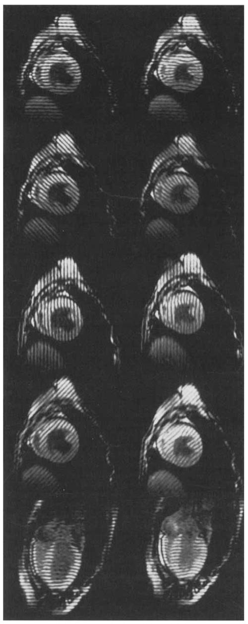
MR images (7.0/2.3, 12° flip angle) of an in vivo canine heart obtained with a parallel tagging and imaging protocol. Two cardiac phases are shown: early and late systole. For each phase, four short axis images and one long axis image is shown: each displays tag lines from a different tag plane orientation.

Strain Reconstruction

A three-dimensional strain map of the LV for each cardiac phase was reconstructed using the DMF algorithm. First, a displacement field was reconstructed from tag lines extracted from the image data (9). A three-dimensional strain tensor was then computed at each of 600 material points in the myocardium. Details of the DMF algorithm are described below. Note that first the tag lines and myocardial contours are tracked for all time frames, then a displacement field is reconstructed for each time frame, and then the strain field is reconstructed for all time frames.

Tag and contour tracking

In each image, the tag lines, endocardial contours, and epicardial contours were tracked with the computer-aided method of Guttman et a1 (19,20). Because the physical location of each slice is known from the imaging protocol, the tag and contour lines can be positioned in three-dimensional space.

Summary of the DMF algorithm

Three-dimensional finite-element mesh construction

To use the finite difference reconstruction technique described below, the LV wall was decomposed into a uniformly spaced three-dimensional mesh. First, a Cartesian coordinate system was constructed in which the x and y directions correspond to the horizontal and vertical directions in a short-axis image and the positive z direction is normal to the x and y directions and points from apex to base. Then, for each imaged cardiac phase, a three-dimensional bounding box aligned with the coordinate system described above was computed that encloses the epicardial and endocardial contours. Each bounding box was subdivided into a regularly spaced three-dimensional mesh of points as shown in Figure 2a. We call this mesh the spatial point grid. The spatial point grid spacing must be chosen small enough so that the algorithm can reconstruct small fluctuations in the displacement field. Choosing the grid spacing too small, however, results in an unnecessary increase in computation time. We have found that a grid spacing of 1.0 mm results in a good tradeoff between these two considerations (9). A 1.0-mm spacing results in a grid of 84 × 84 × 90 points.

Figure 2.

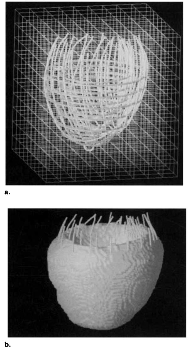
Finite difference mesh construction. The small circles are septal and apical landmarks. (a) A bounding box was constructed around the LV contours extracted from the image data and subdivided into mesh with a 1.0-mm spacing (the mesh shown has a 8.0-mm spacing). (b) The LV wall is a subset of mesh points, which were selected using shape-based interpolation.

The LV wall is defined by a subset of the spatial point grid as shown Figure 2b. These points were selected by shape-based interpolation (21) using all of the contours in the cardiac phase.

Spatial coordinate displacement fit

The end-diastolic location of each material point described above was determined by computing a spatial coordinate displacement field for each cardiac phase, which maps each point in the deformed LV wall back to its end-diastolic location.

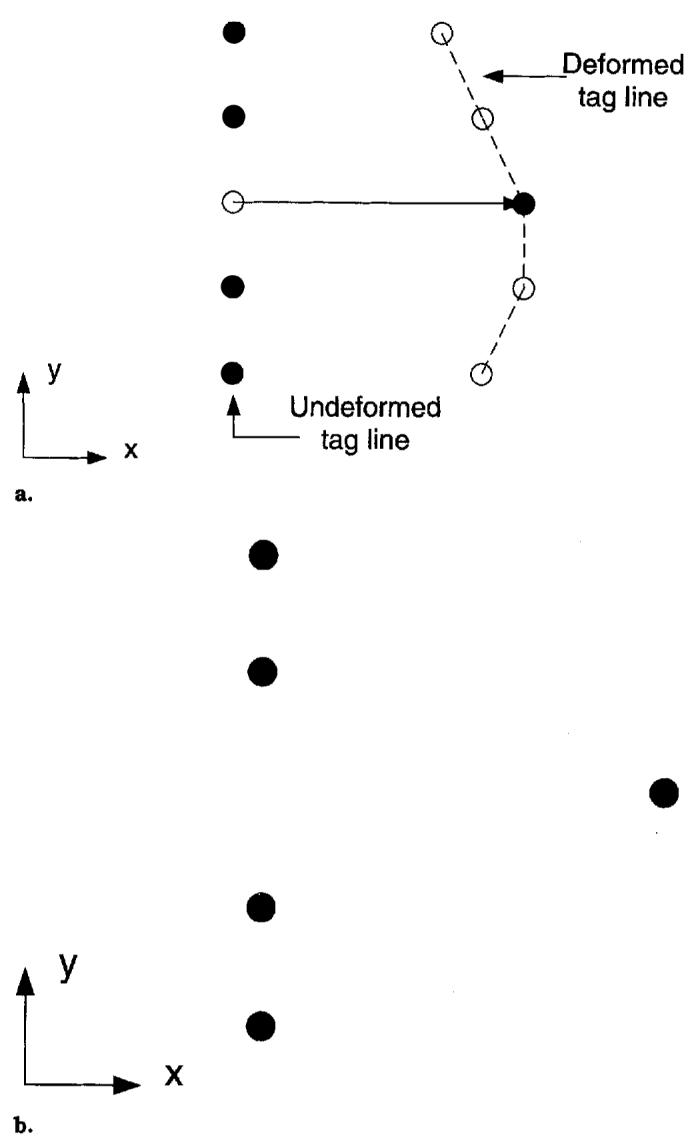
The end-diastolic (ie, undeformed) location of each tag plane was determined from the imaging protocol, and for each point on a deformed tag line, the one-dimensional displacement of the point in the direction normal to the undeformed tag plane was computed as shown in Fig. 3. These one-dimensional displacements are a set of constraints that the spatial coordinate displacement field must satisfy. Displacement constraints in different directions are obtained by acquiring images with different tag plane orientations. At least three different directions are needed to reconstruct a three-dimensional displacement field. The one-dimensional constraints from all directions can be stacked to form the matrix equation (cf, ref. 9)

$$Y=\mathit{EU}+W.$$ [1]

Y is a vector containing the one-dimensional displacements, E is a matrix containing the undeformed tag plane normals, U is a vector containing all of the three-dimensional displacement vectors to be estimated in a given time frame, and W is a zero mean noise vector with covariance matrix ${\sigma }_w^{2}I$, which models any errors in the tag line tracking algorithm. Small values of ${\sigma }_w^2$, correspond to small errors in tag tracking.

Figure 3.

Displacement field measurements from planar tagged images. The material point at the spatial point r on the tag line originated off the image plane at the point p on the undeformed tag plane. Only the displacement vector u in the direction of the tag plane normal e is known.

Because of the relatively small spatial point grid spacing, there are many more unknown displacement vectors than tag line constraints, and a smoothness constraint is required to reconstruct U. We used the smoothness constraint

$$E_s\left(u\right)=\int \underset{\mathit{ij}}{\Sigma }{\left[\frac{\partial u_i}{\partial x_j}\right]}^2\mathit{dx},$$ [2]

where u_i and x_i are the ith components of the spatial coordinate displacement field and the spatial coordinate position vector, respectively. This smoothness constraint minimizes the spatial variation of the displacement field. This smoothness constraint can be modeled by setting the differences between pairs of displacement vectors on the spatial point grid equal to zero mean random variables. These differences can be stacked to form the matrix equation SU = V (see ref. 9 for details), where S is a matrix in which each row contains a 1 and a −1 in the appropriate columns and the remaining elements are zero. V is a vector of zero mean random variables with covariance matrix ${\sigma }_s^{2}I$ that models the spatial change in displacement between two neighboring grid points. Small values of ${\sigma }_s^2$ correspond to a spatially smooth displacement field. Large values of ${\sigma }_s^2$ correspond to a relatively rough displacement field.

The linear minimum mean-square estimate of U from the displacement and smoothness constraints was obtained by solving the following linear system:

$$[{\alpha }^2{S}^{T}S+E^{T}E]U=E^{T}Y,$$ [3]

where ${\alpha }^2={\sigma }_w^2∕{\sigma }_s^2$ is a weighting parameter that controls the smoothness of the resulting estimate. Small values of α² give more weight to the tag line measurements and result in a reconstructed displacement field with higher spatial resolution but more sensitivity to noise. Large values of α² give more weight to the smoothness constraint and result in lower spatial resolution but less sensitivity to noise.

The optimal α² for a given data set is not known a priori. For in vivo data, a different α² is chosen for each time frame based on the root-mean-square (RMS) error between tag lines deformed using the reconstructed displacement field and the tag lines extracted from the image data (8). We call this error the “RMS tag line error.” The α² values for each time frame in this study are listed in Table 1. A selection of points from the reconstructed displacement field at the end-systolic time frame (time frame 5) is shown in Fig. 4a. The tail of each vector corresponds to a material point on the deformed myocardium, and the tip shows the estimate of where this point came from at end diastole. Note that the vector tails are along the deformed tag line.

Table 1.

Smoothing Parameter (α²) and RMS Tag Line Error for Each Time Frame

Time Frame	α2	RMS Tag Line Error (mm)
0	.15	.19
1	.15	.19
2	.15	.23
3	.50	.32
4	.50	.34
5	.50	.35

Note.—The RMS tag line error was computed over 18,125 tag points distributed across the myocardium and was spatially invariant.

Figure 4.

A selection of vectors from reconstructed displacement fields. The LV contours and tag lines are shown for reference. The small circles are septal and apical landmarks. (a) Spatial coordinate displacement field. The tail of each vector corresponds to a material point on the deformed myocardium, and the tip shows the estimate of where this point came from at end-diastole. Note that the vector tails are along the deformed tag line. (b) Material coordinate displacement field. The tail of each vector corresponds to a material point on the end-diastolic myocardium, and the tips shows the estimate of where this point is located at end systole.

Material coordinate displacement reconstruction

The spatial coordinate displacement field establishes the end-diastolic location of a set of material points. These material points are different for each cardiac phase. It is useful, for analysis, to map the material points tracked in each cardiac phase to a common end-diastolic grid, which we call the “material point grid.” For each cardiac phase, linear interpolation was used within each 1 × 1 × 1 mm grid cell to map the irregularly spaced material points onto the material point grid (9). The result is a “material coordinate displacement field” for each cardiac phase that maps each point on the material point grid to its deformed location. A selection of displacement vectors from the end-systolic material coordinate displacement field is shown in Fig. 4b. The tail of each vector corresponds to a material point on the end-diastolic myocardium, and the tip shows the estimate of where this point is located at end-systole.

Strain computation

For each cardiac phase, a three-dimensional strain field was computed from the material coordinate displacement field. First, a material point mesh consisting of 3 radial points, 20 circumferential points, and 10 longitudinal points was constructed from the time frame 0 contour data. We call this mesh the “strain mesh.” The displacement gradient was computed at each point on the strain mesh from the material coordinate displacement field by using a forward difference derivative approximation in each direction averaged over a 2 × 2 × 2 mm neighborhood. The difference interval was 1.0 mm. The displacement gradient tensor g is defined as

$$g_{\mathit{ij}}=\frac{\partial u_i}{\partial X_j},$$

where u_i and X_i are the ith components of the material coordinate displacement field and material coordinate position vector, respectively. The Lagrangian strain tensor ε (22) was computed from the displacement gradient using the following formula:

$$\epsilon =\frac{1}{2}[g^T+g+g^{T}g],$$ [4]

where the superscript T denotes transpose. For viewing purposes, the strain tensor was then transformed to a prolate spheroidal coordinate system defined around the LV long axis.

Effect of Tag Detection Errors

The template matching algorithm for detecting the one-dimensional location of the center of a tag has been shown to be highly accurate (23); with a contrast-to-noise ratio (CNR) between the tag center and background myocardium (“tag CNR”) of 10 and a tag width of 1.5 pixels, the uncertainty in tag center estimation is .1 pixel. The uncertainty in the tag center position has been shown to scale inversely with tag CNR (24). The effect of tag detection errors on the DMF algorithm was studied via Monte Carlo simulation (25). First, a material coordinate displacement field was reconstructed from the original end-systolic (time frame 5) tag line data using the smoothing parameter α² from Table 1. A physiologic noise-free parallel tag data set was then generated by using the reconstructed displacement field to compute the deformed position of each tag line. One-dimensional zero mean Gaussian noise was then added to the tag line data, and then a strain field was reconstructed as described above for 200 trials. A strain error was computed at each point in the strain mesh by subtracting the strain tensor computed from the noise-free data set from the tensor computed from the noisy data set. This procedure was performed for noise SDs of .1, .25, .5, .75, and 1.0 mm.

Spatial Resolution of the Combined Tagging and Reconstruction Process

The spatial resolution of the combined tagging and reconstruction process was studied by reconstructing a displacement field in response to a displacement cloud. A displacement cloud is a localized change in displacement that is sampled by the tagging process and reconstructed by the DMF algorithm. The smallest cloud that can be sampled and reconstructed to within a certain accuracy (defined in Results section) is a measure of spatial resolution.

First, a material coordinate displacement field was reconstructed from the end-systolic (time frame 5) tag line data (all offsets and angles) using the smoothing parameter α² from Table 1. Next, a set of 48 midwall material points (8 circumferential, 6 longitudinal) equally spaced around the myocardium was selected. For each material point, a synthetic displacement field was generated consisting of a cloud of radially oriented displacement vectors centered at the material point. The displacement of the cloud center was determined from the reconstructed displacement field described above. The other displacement vectors were given a Gaussian roll-off. A synthetic tag line data set was then generated by using the synthetic displacement field to compute the deformed position of each tag line. A displacement field was reconstructed from the synthetic tag line data using the DMF algorithm. The percent magnitude response was computed by dividing the magnitude of the reconstructed center displacement by the magnitude of the original center displacement and multiplying by 100%. This process was repeated for each of the 48 material points and for displacement clouds oriented in the radial, circumferential, and longitudinal directions. The radial and circumferential displacements were parallel to the short-axis image planes and the longitudinal displacements were perpendicular to the short-axis image planes.

Spatial Resolution of the DMF Strain Reconstruction

The cloud experiment in the previous section studied the spatial resolution of the combined tagging and DMF reconstruction process. To study the spatial resolution characteristics of the DMF algorithm itself, a strain field was reconstructed in response to a single displaced tag point. First, a tag line data set was generated with all tag line points in their end-diastolic position, which is known from the imaging protocol. A single tag point was then displaced to its end-systolic (time frame 5) position as shown in Figure 5. A strain tensor was computed at each point in the material point grid from the tag line data set using the method described in the Results section. The single displaced tag point excites a cloud of points in the reconstructed strain field as shown in Figure 6. We defined the spatial resolution as the full width at half maximum (FWHM) of the cloud, where the FWHM was defined as the maximum diameter of this cloud at one-half the maximum magnitude response. For the magnitude of a strain tensor, we used the maximum magnitude principal strain component. Note that this convention is independent of the coordinate system of the reconstruction. In general, the cloud will be irregularly shaped, so for the cloud diameter, we used the maximum width of the cloud measured by a line through the cloud center. For the cloud center, we used the average position of all points in the cloud greater than or equal to one-half of the maximum value. This process was repeated at each of 144 equally spaced material points in the myocardium (3 radial, 8 circumferential, 6 longitudinal). At each material point, the FWHM was computed for tag displacements from the 0° (x direction), 90° (y direction), and long axis (z direction) tag planes.

Figure 5.

Displacement of a single tag point for computing spatial resolution. (a) A single tag point is displaced to its deformed (end-systolic) position. The other tag points are left in their undeformed (end-diastolic) position. (b) Tag line used for reconstruction.

Figure 6.

A section of the LV free wall colored according to maximum principal strain. The strain field was reconstructed in response to a single displaced tag point, the end-diastolic position of which is shown by the black dot. The FWHM of the strain field is 5.5 mm.

To study the amount of smoothing in the reconstruction, we computed the attenuation of the single tag point displacement by the spatial coordinate fit. The attenuation was computed according to the following formula:

$$\frac{\Vert u_t\Vert -\Vert u_r\Vert }{\Vert u_t\Vert }\times 100\%,$$

where ∥u_t∥ and ∥u_r∥ are the magnitudes of the tag point displacement and the reconstructed displacement, respectively. The displacement attenuation is a measure of the sensitivity of the DMF algorithm to isolated changes in the tag line measurements. A perfect reconstruction would result in an attenuation of 0% because u_t = u_r. Smoothing constraints, however, reduce the sensitivity of the DMF algorithm to isolated changes in the tag line measurements, so larger attenuation values correspond to greater smoothing.

• RESULTS

Strain Reconstruction

A three-dimensional strain map was constructed using the DMF algorithm described in the Methods section. The RMS error between tag lines deformed using the reconstructed displacement field and the tag lines extracted from the image data (RMS tag line errors) for the displacement field fit are shown in Table 1. The RMS tag line error was computed over 18,125 tag points distributed across the myocardium and was spatially invariant. Maps of radial thickening (ε_rr) and circumferential shortening (ε_cc) for time frames 0 through 5 are shown in Figures 7 and 8. The ε_rr and ε_cc strains increase in magnitude from apex to base, from the endocardium to the epicardium, and from the septum to the free wall.

Figure 7.

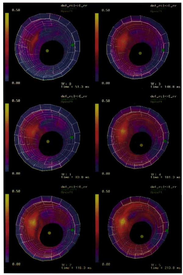
A time sequence of three-dimensional strain maps of radial thickening (ε_rr) of a canine LV. Strains are referenced to a prolate spheroidal coordinate system defined around the long axis of the ventricle.

Figure 8.

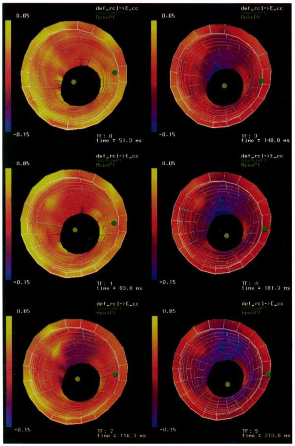
A time sequence of three-dimensional strain maps of circumferential shortening (ε_cc) of a canine LV. Strains are referenced to a prolate spheroidal coordinate system defined around the long axis of the ventricle.

Effect of Tag Detection Errors

The precision of the DMF algorithm was tested using a Monte Carlo simulation as described in the Methods section. The strain error mean and SD for endocardium, midwall, and epicardium material points are plotted versus the SD of the input noise in Figure 9. For each strain component, the error mean and SD was computed over the longitudinal and circumferential points for each radius and all 200 trials. The error statistics for a subset of 100 trials were not significantly different, which suggests that 200 trials were sufficient to obtain stable convergence of the error statistics.

Figure 9.

Mean strain reconstruction error for a canine left ventricle computed over all circumferential and longitudinal points in the mesh shown in Figure 8 and 200 Monte Carlo trials. The error bars correspond to strain error SD. Strains are referenced to a prolate spheroidal coordinate system defined around the long axis of the ventricle. (a) Normal strains: radial–radial (ε_rr), circumferential–circumferential (ε_cc), and longitudinal–longitudinal (ε_ll). (b) Shear strains: radial–circumferential (ε_rc), radial–longitudinal (ε_rl), and circumferential–longitudinal (ε_cl).

For the radial, circumferential, and longitudinal strain, the mean errors are on the order of 3 × 10⁻⁵ for an input noise of .1 mm and increase to roughly .003 at an input noise of 1.0 mm. This small bias in the strain reconstruction is because any error in the reconstructed displacement gradient is squared by the quadratic term (g^Tg) in Equation [4]. The shear strains are not squared by this term, so there should not be a bias in the shear strain reconstruction. This point is reflected in Figure 9, in which the mean strain error stays roughly constant with respect to input noise.

The error SDs for all strain components of radial, circumferential, and longitudinal strains range from roughly .003 for an input noise of .1 mm to .03 at 1.0 mm. These errors should be compared with the strain maps in Figures 7 and 8, in which most of the strains range from roughly .05 to .1 in magnitude. From these results, we conclude that the strain reconstruction has a precision of ±6% for a tag detection accuracy of .1 mm and a tag spacing of 2.5 mm.

Spatial Resolution of the Combined Tagging and Reconstruction Process

The response of the tagging and DMF reconstruction algorithm to a displacement cloud was computed for each of 48 equally spaced midwall material points in the myocardium using the methods described in previously for four different combinations of short axis tag plane angles and tag plane spacings. The mean percent magnitude response is plotted versus l/(cloud width) in Figure 10 for displacement clouds in the radial, circumferential, and longitudinal directions, in which the cloud width is the diameter of the cloud at one-half of its maximum magnitude. The error bars represent ±1 SD. The statistics for each plotted point were computed over the 48 material points. Note that additional short axis tag plane angles have no effect on the longitudinal response because the longitudinal displacements were perpendicular to the short axis image planes.

Figure 10.

Response of the tagging and DMF reconstruction process to a displacement cloud. The error bars represent 1 SD. Statistics are computed over the responses at 48 midwall material points spaced equally around the myocardium. (a) Radially oriented displacement cloud. (b) Circumferentially oriented displacement cloud. (c) Longitudinally oriented displacement cloud.

We interpret the plots in Figure 10 as frequency responses. A measure of spatial resolution was obtained by determining the cloud width that produced a 50% response. The spatial resolutions for each tag configuration and displacement direction are listed in Table 2. The best resolution (5.4 ± .4 mm) was obtained in the circumferential direction when all four tag plane angles and both tag offsets were used. When only two tag plane angles and one offset is used (the minimum required for reconstruction), the resolution drops to 13.1 ± 1.5 mm. Additional tag plane offsets result in a better resolution (8.3 ± .5 mm) than additional tag plane angles (9.1 ± 1.2 mm). In all cases, the circumferential resolution was slightly better than the radial resolution and the longitudinal resolution was significantly more coarse than the in-plane resolution because of the relatively sparse spacing of the long axis image planes relative to the short axis images planes.

Table 2.

Spatial Resolution (in mm) of the Combined Tagging and DMF Reconstruction Process

	Tag Spacing
Tag Angles		5.0 mm	2.5 mm
		Mean ± SD	Mean ± SD
0, 90°	Radial	13.2 ± 1.4	8.6 ±  .5
	Circumferential	13.1 ± 1.5	8.3 ±  .5
	Longitudinal	14.0 ± 4.0	11.0 ± 4.0
0, 90°	Radial	9.1 ± 1.0	5.8 ±  .4
+45°, −45°	Circumferential	9.1 ± 1.2	5.4 ±  .4
	Longitudinal	14.0 ± 4.0	11.0 ± 4.0

Note.—A displacement field was reconstructed in response to a displaced cloud of tag points. Spatial resolution is defined as the cloud width that resulted in a 50% attenuation of the displacement field. Mean and SD are computed over 48 mid-wall material points equally spaced around the myocardium.

Spatial Resolution of the DMF Strain Reconstruction

The spatial resolution of the DMF strain reconstruction was computed for each of 144 equally spaced material points in the myocardium using the methods described previously for four different combinations of short axis tag plane angles and tag plane spacings. The mean, SD, and median resolution were computed over all 144 points and are listed in Table 3. For each case, separate statistics are shown for tag point displacements in the x, y, and z directions and the total over all three directions. The 0, 90°, 5-mm case represents the minimum amount of data required for strain reconstruction. The other three test cases show the change in spatial resolution when offset tag planes, additional short-axis tag plane angles, and both offsets and additional angles are used in the reconstruction.

Table 3.

Spatial Resolution (in mm) of the DMF Reconstruction at End Systole

	Tag Spacing
Tag Angles		5.0 mm		2.5 mm
		Mean ± SD	Median	Mean ± SD	Median
	x	5.68 ± .34	5.75	5.48 ± .32	5.49
0, 90°	y	5.54 ± .33	5.57	5.40 ± .29	5.44
	z	5.82 ± .28	5.88	5.67 ± .32	5.71
	Total	5.68 ± .34	5.74	5.52 ± .33	5.54
	x	5.48 ± .39	5.57	5.25 ± .32	5.25
0, 90°	y	5.36 ± .38	5.43	5.19 ± .32	5.22
+45°, −45°	z	5.81 ± .29	5.87	5.68 ± .32	5.73
	Total	5.55 ± .40	5.60	5.37 ± .39	5.37

Note.—Spatial resolution is defined as the FWHM of the maximum principle strain field in response to a single displaced tag point. The mean, SD, and median were computed over 144 material points spaced equally across the myocardium.

The spatial resolution in the short axis image planes (x and y directions) ranges from 5.6 ± .3 mm (mean ± SD) for the 0, 90°, 5-mm case to 5.2 ± .3 mm when all tag plane angles and offsets are used in the reconstruction. The long axis (z direction) resolution improves slightly from 5.8 ± .3 mm to 5.7 ± .3 mm with an additional set of offset tag planes. The variation in spatial resolution across the myocardium is due to differences in the tag line structure around each displaced tag point. Note that, in contrast to the spatial resolution of the combined tagging and reconstruction process, the spatial resolution of the DMF algorithm itself is relatively insensitive to the tagging geometry.

Table 4 shows statistics for the percent attenuation of the single tag point displacement computed over all 144 material points for the 0, 90°, ±45°, 2.5-mm case. Separate statistics are shown for tag point displacements in the x, y, and z directions and the total over all three directions. An attenuation of 85% means that a displacement vector with a magnitude of 1.0 mm is reconstructed with magnitude of .15 mm. Therefore, larger attenuation values correspond to greater smoothing. Note that although the smoothness constraint in Equation [2] is isotropic, the effective smoothing in the reconstruction is slightly different in each direction because of variations in the tag structure around each displaced tag point.

Table 4.

Attenuation of a Single Tag Point Displacement by the DMF Reconstruction at End Systole for a Tag Spacing of 2.5 mm and Tag Plane Angles of 0°, 90°, and ± 45°

	Mean ± SD	Median
x	87.6% ± 1.8%	87.7%
y	85.0% ± 2.3%	85.6%
z	83.6% ± 3.3%	83.8%
Total	85.4% ± 3.0%	86.0%

Note.—An attenuation of 85% means a displacement vector of magnitude 1.0 mm is reconstructed with a magnitude of .15 mm. The mean, SD, and median were computed over 144 material points spaced equally across the myocardium.

The spatial resolution also is affected by the amount of smoothing used in the reconstruction. The results of a spatial resolution study for the 0, 90°, ±45°, 2.5-mm case using 1/100th the amount of smoothing used in the previous study are shown in Table 5. The mean spatial resolution improves (∼4.5 mm), but the variance increases because the reduction in smoothing results in a reconstruction more sensitive to the tag line data. As in the previous study, there was only a small change in spatial resolution when different combinations of angles and offsets were used in the reconstruction. Because a single displaced tag point is a cloud with zero width, these results can be viewed as an extension of the results in Figure 10, in which the responses for the four tagging geometries get closer together as the cloud width gets smaller.

Table 5.

Spatial Resolution (in mm) of the DMF Reconstruction at End Systole using 1/100th the Amount of Smoothing used in Table 3 for a Tag Spacing of 2.5 mm and Tag Plane Angles of 0°, 90°, and ± 45°

	Mean ± SD	Median
x	4.49 ± .60	4.47
y	4.36 ± .66	4.23
z	4.64 ± 1.09	4.37
Total	4.50 ± .82	4.38

Note.—Spatial resolution is defined as the FWHM of the maximum principle strain field in response to a single displaced tag point. The mean, SD, and median were computed over 144 material points spaced equally across the myocardium.

The decrease in smoothing, however, also affects the noise rejection properties of the DMF algorithm. A Monte Carlo noise analysis using the reduced smoothing resulted in factor of 6 increase in strain errors. From the relatively small change in spatial resolution despite the significant changes in the amount of tag plane data, we conclude that the spatial resolution of the DMF algorithm is determined primarily by the smoothness constraint, but higher levels of smoothing should therefore be used because of their better noise rejection properties.

• DISCUSSION

We have presented a discrete model-free algorithm for reconstructing an accurate, high-resolution three-dimensional strain map of the left ventricle from parallel-tagged MR images. This algorithm decomposes the myocardium into a finely spaced mesh of points and reconstructs a three-dimensional strain map using finite difference analysis and a smoothness constraint that minimizes the spatial variation of displacement across the myocardium. Highly resolved strain reconstruction is possible with this approach because the smoothness constraint is applied to the reconstructed displacement field, and the strain field is left unconstrained.

A three-dimensional strain map also can be reconstructed using finite-element analysis (7,15) or a prolate spheroidal basis function fit (8). These methods, however, require that a specific coordinate system be constructed before the strain map is computed, and in the case of the basis function fit, the accuracy of the fit is highly dependent on the coordinate system used. In addition, the coordinate systems used in (7,8,15) are matched to the geometry of the particular heart being studied and, therefore, require that the entire heart be scanned. Relative to these approaches, the DMF algorithm presented in this paper has the following advantages. First, the DMF algorithm is free of any a priori displacement or deformation models. Second, because of the finite-difference approach, fit accuracy is not dependent on the coordinate system used for the reconstruction.

These advantages have important implications for clinical use of the DMF. Because the DMF does not require a specific heart geometry and produces localized strain estimates, full three-dimensional strain information can be obtained over a localized region of the myocardium from only a few image planes. Imaging these planes would only require one to three breath-hold periods (depending on the performance characteristics of the scanner), which is a reduction in imaging time relative to methods that require the entire volume to be scanned. In addition, the fact that the entire heart is not modeled also implies that the strain computations are not as sensitive to shifts in the position of the heart between breath-holds.

We demonstrated the DMF algorithm on high-resolution parallel-tagged data from an anesthetized dog. The robustness of the strain reconstruction to noise in the tag displacement data was demonstrated with a Monte Carlo simulation. Radial strains were reconstructed from in vivo data with values between .05 and . 1 with a precision of ±.003, for a tag detection accuracy of . 1 mm and a tag spacing of 2.5 mm. Because the tracking accuracy of the Guttman algorithm (19) is on the order of . 1 mm (24), we conclude that the DMF algorithm is accurate enough for clinical assessment of cardiac mechanical function.

The spatial resolution of the combined tagging and reconstruction process was demonstrated by reconstructing a displacement field from tag line data generated by a displacement cloud. When four short axis tag angles and two sets of offset tag planes were used, the spatial resolution was found to be 5.4 ± .4 mm. When compared to the minimum tag configuration of two short axis tag plane angles, one long axis tag plane angle, and no offset tag planes, our results indicate that the acquisition of additional offset tag planes improves the spatial resolution more than acquiring an additional pair of short axis tag plane angles.

The spatial resolution of the DMF algorithm itself was demonstrated by reconstructing a strain field in response to the displacement of a single tag point at 144 points in the myocardium. The FWHM of the strain field reconstructed from a single in-plane tag point was found to be 5.4 ± .3 mm. Our results also show that the FWHM was determined primarily by the amount of smoothing used in the reconstruction and was relatively insensitive to the tagging geometry.

In previous work, Moore et al (26) studied the precision of strains computed by tracking the intersection of radial tags with myocardial contours, and Young et al (27) studied the precision of two-dimensional strains computed using finite element analysis in a deforming phantom. Although both of these studies quantified strain estimate precision, they did not quantify the spatial resolution of the estimates or study the variation in spatial resolution as a function of tag separation and the number of tag plane angles.

Because of the quadratic term in the Lagrangian strain tensor (see Equation [4]), any errors in the displacement reconstruction result in a small positive bias (a tendency to reconstruct strains more positive than the true value) in the rr, cc, and ll strain components. We note that this bias is an inherent property of the Lagrangian strain tensor and will occur regardless of the method used to reconstruct the displacement field. This result suggests that the left (or right) stretch tensor computed from the polar decomposition of the displacement gradient may be a better measure of contractile performance because it does not have the inherent bias of the Lagrangian strain tensor.

The combination of high resolution parallel-tagged MR images and the model-free, coordinate system-free strain reconstruction technique presented in this paper is capable of producing accurate, high resolution strain maps of the myocardium and is a potentially valuable tool in both cardiac mechanics research and in the clinical assessment of cardiac mechanical function.

Abbreviations

CNR

contrast-to-noise ratio

DMF

discrete model free

FWHM

full width at half maximum

LV

left ventricle

RF

radiofrequency

RMS

root mean square

SPAMM

spatial modulation of magnetization

References

- 1.Zerhouni EA, Parish DM, Rogers WJ, Yangand A, Shapiro EP. Human heart: tagging with MR imaging — a method for noninvasive assessment of myocardial motion. Radiology. 1988;169:59–63. doi: 10.1148/radiology.169.1.3420283. [DOI] [PubMed] [Google Scholar]
- 2.Axel L, Dougherty L. MR imaging of motion with spatial modulation of magnetization. Radiology. 1989;171:841–845. doi: 10.1148/radiology.171.3.2717762. [DOI] [PubMed] [Google Scholar]
- 3.Mosher TJ, Smith MB. A DANTE tagging sequence for the evaluation of translational sample motion. Magn Reson Med. 1990;15:334–339. doi: 10.1002/mrm.1910150215. [DOI] [PubMed] [Google Scholar]
- 4.Bolster BD, McVeigh ER, Zerhouni EA. Myocardial tagging in polar coordinates with use of striped tags. Radiology. 1990;177:769–772. doi: 10.1148/radiology.177.3.2243987. [DOI] [PMC free article] [PubMed] [Google Scholar]
- 5.O'Dell WG, Schoeniger JS, Blackband SJ, McVeigh ER. A modified quadrapole gradient set for use in high resolution MRI tagging. Magn Reson Med. 1994;32:246–250. doi: 10.1002/mrm.1910320215. [DOI] [PMC free article] [PubMed] [Google Scholar]
- 6.Fischer SE, McKinnon GC, Maer SE, Boesiger P. Improved myocardial tagging contrast. Magn Reson Med. 1993;28:318–327. doi: 10.1002/mrm.1910300207. [DOI] [PubMed] [Google Scholar]
- 7.Young AA, Axel L. Three-dimensional motion and deformation of the heart wall: estimation with spatial modulation of magnetization — a model-based approach. Radiology. 1992;185:241–247. doi: 10.1148/radiology.185.1.1523316. [DOI] [PubMed] [Google Scholar]
- 8.O'Dell WG, Moore CC, Hunter WC, Zerhouni EA, McVeigh ER. Displacement field fitting for calculating 3D myocardial deformations from parallel-tagged MR images. Radiology. 1995;195:829–835. doi: 10.1148/radiology.195.3.7754016. [DOI] [PMC free article] [PubMed] [Google Scholar]
- 9.Denney TS, Jr, Prince JL. Reconstruction of 3D left ventricular motion from planar tagged cardiac MR images: an estimation theoretic approach. IEEE Trans Med Imaging. 1995;14(4):625–635. doi: 10.1109/42.476104. [DOI] [PubMed] [Google Scholar]
- 10.Cigarroa CG, deFilippi CR, Brickner ME, Alvarez LG, Wait MA, Grayburn PA. Dobutamine stress echocardiography identifies hibernating myocardium and predicts recovery of left ventricular function after coronary revascularization. Circulation. 1993;88(2):430–436. doi: 10.1161/01.cir.88.2.430. [DOI] [PubMed] [Google Scholar]
- 11.Varga A, Picano E, Cortigiani L, et al. EPIC (Echo Persantine International Cooperative) and EDIC (Echo Dobutamine International Cooperative) study groups Does stress echocardiography predict the site of future myocardial infarction? A large-scale multicenter study. J Am Coll Cardiol. 1996;28(1):45–51. doi: 10.1016/0735-1097(96)00112-x. [DOI] [PubMed] [Google Scholar]
- 12.Le Feuvre C, Baubion N, Aubry N, Metzger JP, de Vernejoul P, Vacheron A. Assessment of reversible dyssynergic segments after acute myocardial infarction: dobutamine echocardiography versus thallium-201 single photon emission computed tomography. Am Heart J. 1996;131(4):668–675. doi: 10.1016/s0002-8703(96)90269-0. [DOI] [PubMed] [Google Scholar]
- 13.Elhendy A, Trocino G, Salustri A, et al. Low-dose dobutamine echocardiography and rest-redistribution thallium-201 tomography in the assessment of spontaneous recovery of left ventricular function after recent myocardial infarction. Am Heart J. 1996;131(6):1088–1096. doi: 10.1016/s0002-8703(96)90082-4. [DOI] [PubMed] [Google Scholar]
- 14.Picano E, Ostojic M, Varga A, et al. Combined low dose dipyridamole-dobutamine stress echocardiography to identify myocardial viability. J Am Coll Cardiol. 1996;27(6):1422–1428. doi: 10.1016/0735-1097(95)00621-4. [DOI] [PubMed] [Google Scholar]
- 15.Young AA, Kraitchman DL, Dougherty L, Axel L. Tracking and finite element analysis of stripe deformation in magnetic resonance tagging. IEEE Trans Med Imaging. 1995;14(3):413–421. doi: 10.1109/42.414605. [DOI] [PubMed] [Google Scholar]
- 16.Moulton MJ, Creswell LL, Downing SW, et al. Spline surface interpolation for calculating three-dimensional ventricular strains from MRI tissue tagging. Am J Phys. 1996;270:H281–H297. doi: 10.1152/ajpheart.1996.270.1.H281. [DOI] [PubMed] [Google Scholar]
- 17.McVeigh ER, Atalar E. Cardiac tagging with breath-hold cine MRI. Magn Reson Med. 1992;28:318–327. doi: 10.1002/mrm.1910280214. [DOI] [PMC free article] [PubMed] [Google Scholar]
- 18.McVeigh ER. MRI of myocardial function: motion tracking techniques. Magn Reson Imaging. 1996;14(2):137–150. doi: 10.1016/0730-725x(95)02009-i. [DOI] [PubMed] [Google Scholar]
- 19.Guttman MA, Prince JL, McVeigh ER. Tag and contour detection in tagged MR images of the left ventricle. IEEE Trans Med Imaging. 1994;13(1):74–88. doi: 10.1109/42.276146. [DOI] [PubMed] [Google Scholar]
- 20.Guttman MA, Zerhouni EA, McVeigh ER. Analysis and visualization of cardiac function from MR images. IEEE Comp Graph Appl. 1997;17(1):30–38. doi: 10.1109/38.576854. [DOI] [PMC free article] [PubMed] [Google Scholar]
- 21.Raya SP, Udupa JK. Shape-based interpolation of multidimensional objects. IEEE Trans Med Imaging. 1991;9(1):32–42. doi: 10.1109/42.52980. [DOI] [PubMed] [Google Scholar]
- 22.Spencer AJM. Continuum mechanics. Longman Group Limited; New York: 1980. [Google Scholar]
- 23.Moore CC, Reeder SB, McVeigh ER. Tagged MR imaging in a deforming phantom: photographic validation. Radiology. 1994;190:765–769. doi: 10.1148/radiology.190.3.8115625. [DOI] [PMC free article] [PubMed] [Google Scholar]
- 24.Atalar E, McVeigh ER. Optimization of tag thickness for measuring position with magnetic resonance imaging. IEEE Trans Med Imaging. 1994;13(1):152–160. doi: 10.1109/42.276154. [DOI] [PMC free article] [PubMed] [Google Scholar]
- 25.Press WH, Flannery BP, Teukolsky SA, Vetterling WT. Numerical Recipes in C. Cambridge University Press; 1988. [Google Scholar]
- 26.Moore CC, O'Dell WG, McVeigh ER, Zerhouni EA. Calculation of three-dimensional left ventricular strains from biplanar tagged MR images. JMRI. 1992;2:165–175. doi: 10.1002/jmri.1880020209. [DOI] [PMC free article] [PubMed] [Google Scholar]
- 27.Young AA, Axel L, Dougherty L, Bogen DK, Parenteau CS. Validation of tagging with MR imaging to estimate material deformation. Radiology. 1993;188:101–108. doi: 10.1148/radiology.188.1.8511281. [DOI] [PubMed] [Google Scholar]