Left ventricular motion reconstruction from planar tagged MR images

Abstract

Through recent development of MR techniques, it is now possible to assess regional myocardial wall function in a non-invasive way. Using MR tagging, space is marked with planes which deform with the tissue, providing markers for tracking the local motion of the myocardium. Numerous methods to reconstruct the three-dimensional displacement field have been developed. The aim of this article is to provide a framework to quantitatively compare the performance of four methods the authors have developed. Five sets of experiments are described, and their results are reported. Instructions are also provided to perform similar tests on any method using the same data.

The experiments show that some characteristic properties of the methods, such as sensitivity to noise or spatial resolution, can be quantitatively classified. Cross-comparison of performances show what range values for these properties can be considered acceptable.

1. Introduction

With the development of recent MRI techniques, non-invasive evaluation of regional myocardial wall motion and function is becoming a reality (Guttman et al 1997, McVeigh 1998). One of the methods for this purpose is MRI tagging (Axel and Dougherty 1989, Fischer et al 1994, Mosher and Smith 1990, Zerhouni et al 1988). In tagged MRI, the whole space is tagged with a set of planes (or any spatially encoded pattern) which deform with the tissue, providing non-invasive markers that reflect the local displacement of the myocardium. The intersections of these tagging planes with the imaging plane appear as dark lines in the images (McVeigh 1998, McVeigh and Atalar 1992). Using this technique, motion can be reconstructed and local strain tensors can be derived; strain values have been proven to be a significant indicator of function abnormality (Croisille et al 1999, Moore et al 1999).

Many methods have been proposed to reconstruct 3D motion of the LV from tagged MR images (Declerck 1997, Declerck et al 1998a, 1999, Denney and McVeigh 1997, Huang and Amini 1999, Moulton et al 1996, O’Dell et al 1995, O’Donnell et al 1996, Öztürk and McVeigh 1999a, Park et al 1996, Radeva et al 1997, Young 1998, Young and Axel 1992), and compute 3D strains at material points in the heart wall. All these methods except Huang and Amini (1999), Radeva et al (1997) and Young (1998) suppose that tag lines have been segmented in a preliminary step. A number of methods have been described in the literature to fulfil this time-consuming step, using pattern matching (Denney 1999), snakes (Guttman et al 1994,Radeva et al 1997), or spline modelling (Amini et al 1994, Kraitchman et al 1995, Kumar and Goldgof 1994, Young et al 1995), with a different level of automation, none being fully automatic at this time.

As the information given by the tag pattern is essentially sparse, each method has to define an interpolation scheme so that spatial derivatives (gradients, and therefore, strains) can be computed. In the work of Huang and Amini (1999), Moulton et al (1996), Öztürk and McVeigh (1999a) and Radeva et al (1997), the deformation is modelled with B-spline tensor products in Cartesian space, with some variety in the way they are estimated from the data. In Declerck et al (1998a, 1999) and O’Dell et al (1995), the deformation is also modelled using Legendre polynomial or B-splines, but in a particular polar geometry (planispheric or prolate spheroidal respectively). In those methods, the shape of the LV is not modelled as a geometric object, but the deformation space is defined in prolate spheroidal coordinates which are roughly adapted to the shape of the LV. On the contrary, in the work of O’Donnell et al (1996), Park et al (1996), Young and Axel (1992) and Young (1998), the LV-shape is approximated with a model on which finite elements bases are defined to generate a continuous deformation: volumic superquadric with parametric offsets in O’Donnell et al; volumic deformable superquadric in Park et al; or 16-element cubic polynomials in Young’s work. Only the work of Denney and McVeigh (1997) gives a method other than the approximation of the displacement field by a continuous function. In this method, the myocardial wall is decomposed into a finely spaced mesh where displacement at each node is constrained via finite difference analysis by a smoothness constraint. Between nodes of the mesh, the displacement field is approximated using linear interpolation, but the noise modelling in the smoothness constraint is a very important part of the characteristic of the deformation model.

Each of the interpolation procedures described above uses an LV deformation model. Therefore, for a given dataset, the resulting strain computed through this modelling will be different for each method. In order to try to quantify the differences between these methods and comment on some of their characteristic features, we present in this paper the results of a series of experiments in order to compare four methods. In chronological order of publication, those methods are:

• tag strain (E) analysis (TEA) (O’Dell et al 1995)

• discrete model-free (DMF) (Denney and Prince 1995)

• four-D tag strain (E) analysis (FTEA) (Declerck et al 1998a, 1999)

• tag tissue tracker (TTT) (Öztürk and McVeigh 1999a).

All of these methods suppose pre-segmentation of the tag lines, which is provided for instance by the FindTags package (Guttman et al 1994). The choice of these methods was motivated by the variety of techniques they use; this variety is also representative of all the possibilities represented in the literature—LV-specific or not, discrete or continuous in space, incorporating a time dependency constraint or not. Though this choice is restrictive and arbitrary, the experiments which are described in this paper design a framework for whoever desires to compare another method with these four.

The paper is organized as follows: in section 2, we give a short description of the methods we compare in this article. In section 3, we describe the different experiments we process for the comparison, and we draw conclusions based on the results of the experiments in section 4.

2. Theory: description of the four reconstruction methods

We recall here the main ideas of the displacement field reconstruction methods. Further details are available from the references. Using three perpendicular tag orientations, two perpendicular to the short-axis (SA) planes and one perpendicular to the long axis (LA) (McVeigh 1998, McVeigh and Atalar 1992), all four methods compute the backward displacement field ${\mathit{f}}_n^{\text{back}}$ between a time t_n and the reference tagging time t_T (figure 1). The backward displacement field ${\mathit{f}}_n^{\text{back}}$ is then inverted into f_n for each time frame for 3D methods (DMF, TEA), or into f with a continuous time parametrization for 4D methods (TTT, FTEA). The displacement can therefore be computed on material points over the sequence.

Figure 1.

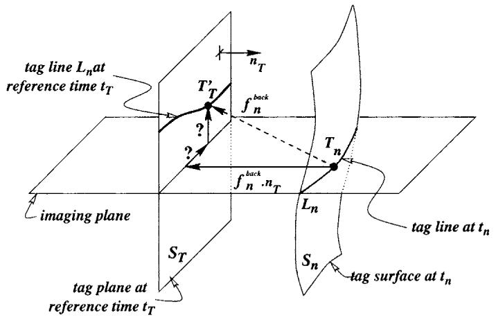
The tag plane at tagging time S_T deforms into surface S_n at time t_n. The backward transformation ${\mathit{f}}_n^{\text{back}}$ deforms S_n back onto S_T. A tag point T_n of a tag line L_n was a point $T_T^{\prime }$ in S_T at tagging time t_T, which gives a one-dimensional constraint on the displacement. Using three independent tagging directions n_T makes the estimation of ${\mathit{f}}_n^{\text{back}}$ possible.

In the following, the methods which model only the backward transformation (DMF, TEA) are presented first, then follow the descriptions of the methods which perform a computation of the forward transformation (TTT, FTEA):

1. Backward transformations

   DMF: Cartesian

   TEA: polar.

2. Forward transformations

   TTT: Cartesian

   FTEA: polar.

2.1. 3D inverse methods

2.1.1. DMF: discrete model-free

The discrete model-free (DMF) algorithm (Denny and Prince 1995) uses finite difference analysis to reconstruct displacement and strain from tag lines and user-defined myocardial contours. For each imaged time frame, the DMF first constructs a 3D segmentation of the LV wall on a regularly spaced discrete grid of points from the user-defined endocardial and epicardial contours. The grid spacing is equal to the pixel size in the MR image. A displacement vector is estimated for each grid point in the LV segmentation that maps the grid point back to its end-diastolic position. Defining $U_n^{\text{back}}$ to be a vector containing all the displacement vectors at time t_n to be estimated (this $U_n^{\text{back}}$ compiles all the evaluations of $u_n^{\text{back}}={\mathit{f}}_n^{\text{back}}-\mathbf{Id}$ at the grid points, Id designating the identity), the one-dimensional displacement constraints obtained from the tag line data can be written as the matrix equation $D_n^{\text{back}}={\mathit{EU}}_n^{\text{back}}$, where $D_n^{\text{back}}$ is a vector containing the one-dimensional tag displacements and E is a matrix containing the undeformed tag plane normals. Since the grid spacing is small compared with the tag line spacing, there are many more unknown displacement vectors than tag line constraints, and a smoothness constraint is required to reconstruct $U_n^{\text{back}}$. DMF uses the smoothness constraint:

$${\epsilon }_s\left(u\right)=\int \sum _{ij}{\left[\frac{\partial u_i}{\partial x_j}\right]}^2\mathrm{d}x$$ (1)

where u_i and x_i are the ith components of the spatial coordinate displacement field u = f-Id and the spatial coordinate position vector x respectively. The smoothness constraint in equation (1) minimizes the spatial variation of the displacement field, it can be modelled by setting the differences between pairs of displacement vectors on the spatial point grid equal to zero mean random variables. These differences can be stacked in the matrix equation ${\mathit{SU}}_n^{\text{back}}=V$, where S is a matrix in which each row contains zeros except a 1 and a -1 in the appropriate column (see Denney and Prince (1995) for more details). V is a vector-with zero mean random variables with scalar covariance matrix that models the spatial change in displacement between two neighbouring points.

The linear minimum mean-square estimate of $U_n^{\text{back}}$ from the tag line and smoothness constraints is then obtained by solving the following linear system

$$[{\alpha }^2{S}^{T}S+E^{T}E]U_n^{\text{back}}=D^T{D}_n$$ (2)

where α² is a weighting parameter that controls the smoothness of the resulting estimate. Small values of α² give more weight to the tag line measurements and result in a reconstructed displacement field with higher spatial resolution but more sensitivity to noise. Large values of α² give more weight to the smoothness constraint and result in lower spatial resolution but less sensitivity to noise. For all experiments in this paper, we used empirically determined values of α² = 1 at early systole gradually decreasing to α² = 0.134 at end systole (0.134 being the inverse of the corresponding time slot; see Denny and Prince (1995) for more details).

Strain is computed by first converting the reconstructed displacement field to material coordinates using linear interpolation. The displacement gradient is then computed using a finite difference derivative approximation averaged over a 3 × 3 × 3 point neighbourhood. Finally the Langrangian strain tensor is computed from the displacement gradient.

2.1.2. TEA: tag strain (E) analysis

For the 3D reconstruction of $u_n^{\text{back}}$, we use a series expansion expressed in a dimensionless prolate spheroidal coordinate system [λ*,φ,θ]. λ* represents wall depth and has values of zero at midwall, -0.5 at the endocardial surface, and 0.5 at the epicardial surface. φ, θ represent azimuthal and circumferential angles, respectively. Using analogy to the spherical harmonic series (Press et al 1992), displacement in the radial coordinate direction, λ, can be represented as

$$\delta \lambda =\sum _{r=0}^{n^r}{(\lambda \ast )}^r\sum _{l=0}^{n^l}\sum _{m=-1}^l{a}_{r,l,m}{P}_l^{\mid m\mid }\left(\cos \left(\phi \right)\right)\{\begin{array}{cc}\sin \left(m\theta \right)\hfill & m>0\hfill \\ \cos \left(m\theta \right)\hfill & m\le 0.\hfill \end{array}\phantom{\}}$$ (3)

$P_l^m$ are the associated Legendre polynomial functions and a_r,l,m the unknown coefficients. The number of terms included in the series expression is given by the parameters n^r and n^l. Similar expressions are used to model the angular displacement in the longitudinal and circumferential directions, δφ and δθ. The measured displacements in X, Y and Z directions are projected onto the local prolate spheroidal coordinate unit vectors and the δλ, δφ and δθ series coefficients are determined simultaneously.

The backward displacement field is inverted at the points where the strain is computed using a gradient descent approach. Iterations are stopped when an arbitrary precision is reached.

The fit to the prolate spheroidal coordinate-based model is preceded by a correction for the bulk motions of the ventricle. This is necessary because the origin and long axis of the prolate spheroidal coordinate system are singularity points which should be kept out of the myocardium.

This 3D kinematic model functions to interpolate the myocardial motion between samples in space, to filter out noise in the sampled data and to facilitate the computation of the local displacement gradients used for strain calculation. In our experiments, we choose n^r = 1 and n¹ = 5.

2.2. 4D forward methods

2.2.1. TTT: tag tissue tracker

Initially, for each short axis image plane (i), time frame (n) and short axis tag stack (s), a two-dimensional B-spline field is formulated to approximate the one-dimensional displacement of a tag surface:

$$d_{n,i,s}^{\text{back}}=\sum _u\sum _v{B}_u\left(x\right)B_v\left(y\right)C_{n,i,s,u,v}^{\text{back}}.$$ (4)

In the above equation, d^back is the one-dimensional tag displacement from t_n to t_T, B is the B-spline basis function, x and y are image coordinates, u and v, the B-spline parameter directions and C^back refers to control point values. Summation is done over all the defined control point 2D tensor products for a given image location. Cubic splines with a homogeneous know sequence in each direction (Farin 1989) and a 10 × 10 control point density are used in this study and are estimated by least-squares minimization.

Once we calculate displacement fields of both tag stacks at a given short-axis image plane and time frame, we can determine two components of the past total trajectory of any tag point. The final inverse motion field should give for each point the 3D vector pointing to its reference material point at the undeformed state. The missing component, the SA through-plane motion, is computed from LA images as follows: (a) a 2D B0-spline field is fit for the displacement on each long axis imaging plane; (b) this parametric field is then evaluated at each SA image plane intersection line; (c) through-plane displacement information coming from all LA images is used to fit a second field in each SA plane.

If care is taken to use the same region of interest in both SA tag displacement field fitting and the last step of long-axis analysis, we can describe a single formula for a B-spline inverse deformation field:

$$D_{n,i}^{\text{back}}=\sum _u\sum _v{B}_u\left(x\right)B_v\left(y\right)\left[\begin{array}{c}\hfill C_{n,i,1,u,v}^{\text{back}}\hfill \\ \hfill C_{n,i,2,u,v}^{\text{back}}\hfill \\ \hfill C_{n,i,3,u,v}^{\text{back}}\hfill \end{array}\right].$$ (5)

This similar to equation (4), but the final displacement $D_{n,i}^{\text{back}}$ is now a vector. For each time frame (n), using equation (5) three-dimensional inverse displacement vectors $D_{n,m}^{\text{back}}$ of all short-axis tag points T_n,m are calculated. The forward deformation U_n,m at the corresponding point at tagging time should be the inverse (-D_n,m).

The forward deformation u_n = Id as a three-dimensional B-spline tensor product for a given time frame (n) can be described, for a material point x, as:

$$u_n\left(x\right)=\sum _u\sum _v\sum _w{B}_u\left(x\right)B_v\left(y\right)B_w\left(z\right){\left[C_n\right]}_{u,v,w}.$$ (6)

In this equation, the sum for a given material point is done over the entire defined 3D tensor product of basis functions and control points [C_n]. As for the inverse case, cubic B-splines are used and control density is chosen as 8 × 8 × 8.

After 3D forward deformation field is constructed for each time frame, a 1D time smoothing is performed on control points. For this time smoothing we use cubic splines and a number of control points equal to 60% of the number of time frames. We now describe the motion of the heart as a four-dimensional B-spline forward motion field as

$$u(x,t)=\sum _v\sum _v\sum _w\sum _t{B}_u\left(x\right)B_v\left(y\right)B_w\left(z\right)B_t\left(t\right)C_{u,v,w,t}$$ (7)

u being the displacement f - Id.

In this equation, the sum for a given point in space and time is done over the 4D tensor product of the basis functions and the control points.

2.2.2. FTEA: four-D tag strain (E) analysis

The backward transformations ${\mathit{f}}_n^{\text{back}}$ deforms a point x onto a point for which the coordinates are defined as a tensor product of B-spline curves (Declerck et al 1995, 1997), as for the B-solid defined in (Radeva et al 1997) or for the forward transformation in TTT:

$${\mathit{f}}_n^{\text{back}}\left(x\right)=\sum _{i=0}^{n^x-1}\sum _{j=0}^{n^y-1}\sum _{k=0}^{n^z-1}{\left[C_n^{\text{back}}\right]}_{i,j,k}{B}_i^x\left(x\right)B_j^y\left(y\right)B_k^z\left(z\right)$$ (8)

where we define $C_n^{\text{back}}$ as the set of 3D control points, and for the x coordinate for instance, $B_i^x$ the ith cubic B-spline basis function of degree K and n_x the number of control points (Farin 1989).

The transformation is estimated by minimizing a criterion which is the weighted sum of the two following terms:

1. A data term, which is the sum of square distances of each deformed tag points from its tagging plane. This term incorporates equally all tag displacement constraints at once.

2. A smoothing term, which is the integral of the square of the second derivatives of ${\mathit{f}}_n^{\text{back}}$.

The criterion is quadratic in the control points ${\left[C_n^{\text{back}}\right]}_{i,j,k}$. We are therefore guaranteed to find the unique global minimum provided the criterion is positive definite. In our implementation, the criterion is minimized with a conjugate gradient method, and the number of control points is set to 8 × 8 × 8.

The transformations ${\mathit{f}}_n^{\text{back}}(n=0\dots T-1)$ are estimated sequentially, using ${\mathit{f}}_{n-1}^{\text{back}}$ as the initial transformation for the conjugate gradient (identity for n = 0). With all ${\mathit{f}}_n^{\text{back}}$, we compute a 4D planispheric transformation (Declerck et al 1998b). For a material point x, we define two angles θ, φ and a distance r as for the prolate spheroidal system. The planispheric coordinates (X, Y, R) are expressed as follows:

$$\begin{array}{c}X=\frac{\theta }{\pi }\cos \left(\phi \right)\hfill \\ Y=\frac{\theta }{\pi }\sin \left(\phi \right)\hfill \\ R=\frac{r}{{\sigma }_r}\hfill \end{array}$$ (9)

where σ_r is such that X, Y and Z are dimensionless numbers of the same range. These planispheric coordinates are deformed by f with the following scheme:

$$\begin{array}{c}{X}^{\prime }=a_{0}X-a_{1}Y+a_2\hfill \\ Y^{\prime }=a_{1}X+a_{0}Y+a_3\hfill \\ R^{\prime }=a_{4}R+a_5\hfill \end{array}$$ (10)

where a_0...5 are B-spline tensor products of time and space. The equations in X and Y are a 2D local similarity transform (a uniform scaling, a rotation and a translation) and the equation in R is a local affine: Declerck et al (1998b) describes how these equations (10) are related to the local motion of the myocardium as it contracts (wall thickening, long-axis twist and shortening).

To compute f, we use the series of pairs of matched points between time t_T and each time frame t_n that all the computed ${\mathit{f}}_n^{\text{back}}$ provide. For each n, each tag point T_n,m is matched to its deformed tag point at t_T, which is estimated as being ${\mathit{f}}_n^{\text{back}}\left(T_{n,m}\right)$. This point should be transformed by f into T_n,m itself. We thus can write a least-squares criterion to estimate f as follows:

$$\epsilon \left(\mathit{f}\right)=\sum _n\sum _m{\alpha }_{n,m}d{(\mathit{f}({\mathit{f}}_n^{\text{back}}\left(P_{n,m}\right),t_n);P_{n,m})}^2$$ (11)

where d(·; ·) is the distance and α_n,m a weighting coefficient whose value is related to the reliability of the pair $[({\mathit{f}}_n^{\text{back}}\left(T_{n,m}\right),t_n);T_{n,m}]$ (chosen as 1 in our experiments). Minimizing ε for f is done identically as in Declerck et al (1998b).

2.3. Summary of features for the four methods

We summarize here in table 1 the characteristic features of the four methods, including some characteristic computational times, for a typical sequence of 12 images, on a state-of-the-art workstation (250 MHz).

Table 1.

Summary table of the features of the four methods.

	Method
Feature	DMF	TEA	TTT	FTEA
LV-specific		X		X
Polar coordinates		X		X
Cartesian coordinates	X		X
Discrete	X
Backward fit only	X	X
Backward and forwards fits			X	X
Time constrained (4D)			X	X
Computational time	70 min	40 min	30 min	40 min

2.4. Uniformity of data processing

Before starting the experiments, we need to make sure that the method will be processed on the same data and the strain computation will be computed on the same material points. Due to the generation of the tag pattern, there is a delay between the detection of the peak of the R wave and the acquisition of the first image (9.2 ms with our pulse sequence). Each image is acquired during 35 ms (11 lines of k-space with TR = 3.1 ms). Therefore, between the first point and the last point acquired in k-space, there is a delay of 35 ms which is enough for the heart to move a few millimetres. So the tag points which one detects on the first time frame are slightly deformed and are not on perfectly parallel planes. It is therefore necessary to compute the equations of the tag planes in order to write the 1D constraints on the displacement field (figure 1). None of the methods we cite from the literature describe how to compute these equations, so we insert this procedure in this paper, as there may be multiple methods for doing so. Second, as the strain is generated on material points inside the myocardium, we explain the method we use to generate the material points mesh used by all four reconstruction methods.

2.4.1. Reconstruction of tag planes

In this study the tag plane pattern is fully defined once we know the normal of the tag plane, the spacing between consecutive tag planes and the position of one point in a plane (an offset position). In the protocol we used for imaging (McVeigh 1998, McVeigh and Atalar 1992), the tag normal is reliable (it is parallel to the readout gradient), but the tag spacing is not. As a matter of fact, we noticed a difference of around 2% in the tag spacing obtained from the images in non-moving parts of the body (liver, etc) and the expected tag spacing computed from the pulse sequence, due to a slight error in the implementation of the pulse sequence on the scanner.

The planes are approximated with a least-squares fit from the points in the myocardium at time t₀ (first time slot). The normal to the tag planes is known from the image headers written by the scanner. The motion of the heart during the 9.2 ms duration of the tag sequence generation is neglected.

2.4.2. Heart wall mesh generation

The mesh generation is done using the method of the TEA program. The contours generated in the segmentation program (FindTags) are parametrized in prolate spheroidal coordinates. Each material point x has prolate spheroidal coordinates (λ, θ, φ). The endocardial and epicardial surfaces are approximated by fitting a spherical harmonic surface (Press et al 1992) as a function of the two angles θ and φ:∧ (θ, φ). This approximation allows us to render a smooth but reliable surface of the LV wall. Some points are chosen along this surface for a discrete set of θ and φ for the analysis. By differentiating the equation of Λ(θ, φ), it is possible to generate the tangent and normal vector to the surfaces, and therefore to define local radial, circumferential and longitudinal directions, which set a local coordinate system we use for the strain analysis.

3. Experimental methods

In this section we develop the protocol we used to test the different methods. Ideally, we would proceed using a synthetic heart motion, but unfortunately, all simulators we found in the literature (Arts et al 1992, O’Dell et al 1995, Waks et al 1996, Young 1998) use a prolate spheroidal coordinate system to define the motion. As one of our methods (TEA) also uses the prolate spheroidal coordinate system, it obviously has an advantage under these circumstances and any comparison would have been biased. Therefore, the experiments were done on real data.

First, to assess the agreement between the motion reconstructions on the same data, we computed the strain tensor on a normal heart where particular care was taken to estimate the tag point locations. This dataset had the minimum possible outliers or errors in the tag detection procedure due to repeated manual tuning of the segmentation. For this reason, it will be named the ‘golden’ dataset: it is not as ideal as a synthetic motion for which displacement and strain are exactly known (this would be a ‘gold’ standard), but it is a very low-noise representation of the motions each of the methods will need to model.

The next two experiments were designed to assess the sensitivity to noise and the spatial resolution of the methods. These can show the sensitivity to high or low spatial frequency of deformation: this way, one can deduce the sensitivity of the displacement and strain computation with respect to the tag detection software.

A round robin of tests was also performed using the ‘golden’ dataset to cross-validate the reconstruction methods. Each method is used to generate a displacement field which is approximated using the other methods. These motions are as close as each method can provide of a realistic motion of an LV. We then use these four synthetic heart motions to perform quantitative comparison on displacement and strain distributions.

3.1. Strain maps on a normal heart

In the first experiment, we computed the strain tensor using the four methods on the ‘golden’ dataset: the dataset comprises nine short-axis slices (slice thickness of 8 mm, no gap) and six long-axis slices. Figure 2(a) displays the geometry of the image planes in three-dimensional space.

Figure 2.

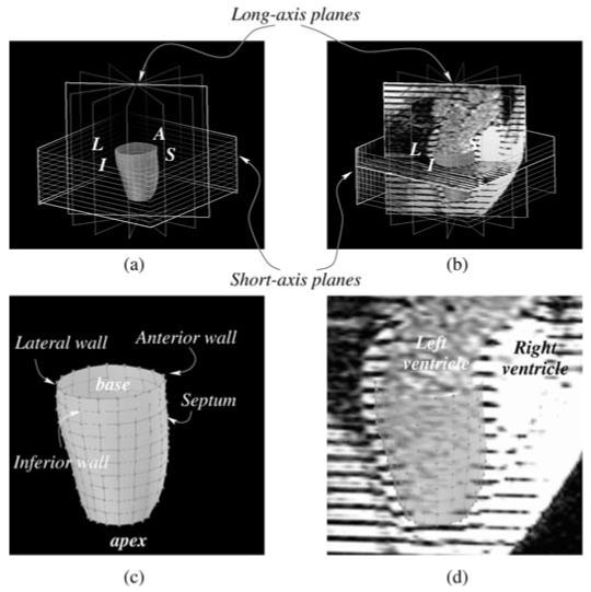
(a) The image planes for short- and long-axis data are shown, with the mesh generated for the golden dataset experiment. L stands for lateral wall, I for inferior, S for septum and A for anterior. (b) The same as (a), with some images included. One can see on the long-axis image, the left and right ventricles, the left atrium and the aortic outflow tract. (c) An enlarged view of (a), with anatomical description of each part of the mesh. (d) An enlarged view of (b), with anatomical description on the long-axis image. The mesh is shown in transparency.

For this dataset, an 11 × 18 cylindrical mesh is generated in the midwall using 18 regular subdivisions in the short-axis (circumferential) planes and 11 subdivisions along the long axis (figure 2). For clarity, only one point out of two in circumferential (9 instead of 18) and one point of two in longitudinal directions (6 instead of 11) will have its strain tensor displayed on the strain maps.

The strain tensor E is the Lagrangian strain tensor rotated in local coordinates in order to fit with the local geometry of the myocardium. The radial direction r is oriented from endocardium to epicardium, the circumferential and longitudinal directions c and l follow the mid-wall contour in the short-axis and long-axis directions respectively. The components of the tensor are written E_ab, where a and b are the directions r, c or l. To make the names easy to understand, the circumferential strain design E_cc, the radial strain E_rr, and the longitudinal strain E_ll. Unless specified otherwise, we concentrate on E_cc which has been proven to be a significant parameter to assess myocardial contractility and function (Croisille et al 1999, Moore et al 1999).

3.2. Noise immunity

The tag detection method defined in Guttman et al (1994) has been shown to be accurate (Moore et al 1994): with a contrast-to-noise of 10 between the tag centre and background myocardium (tag CNR), a tag width of 1.5 pixel, the uncertainty in the estimation of the tag centre point is 0.1 mm. This uncertainty has been shown to be inversely proportional to the tag CNR (Atalar and McVeigh 1994). In order to assess the effect of tag detection uncertainty on the different methods, we study the error of each reconstruction with Monte Carlo simulations (Press et al 1992), as in Denney and McVeigh (1997).

We used the two extreme time frames of the golden dataset: at end-diastole and end-systole: the tag points at end-diastole and end-systole are perturbed with 1D Gaussian noise with a chosen standard deviation σ perpendicular to the direction of the tag plane normal. The displacement field is then reconstructed for each method for 200 trials. The displacement vector and strain tensors are computed for each point in the midwall mesh and subtracted to the noise-free displacement vector and strain tensor, computed from the original tag points at end-diastole and end-systole. The mean and standard deviation of the difference is computed over all the points on the mesh for all trials. This experiment is processed for noise σ of 0.1, 0.2, 0.3 and 0.4 mm.

This test was run only to assess sensitivity to spatial noise in the reconstruction of the motion. For the 4D methods FTEA and TTT, we do not take into account their capacity of interpolation between time frames and they are run as if they were 3D methods (exact time interpolation at end-diastole and end-systole).

3.3. Spatial resolution

To assess spatial resolution for each method, ‘cloud’ experiments were done as in Denney and McVeigh (1997), by reconstructing a displacement field in response to a displacement cloud. The smallest cloud that can be reconstructed with a certain accuracy (to be defined) is a measure of the spatial resolution. This method is analogous to defining the modulation transfer function of an imaging system.

A synthetic displacement field is generated as a local displacement of a point (the centre C of the cloud) towards a point D. Neighbouring points to the centre are also moved in the same direction d = CD/||CD||, the amplitude of the displacement is defined with a Gaussian roll-off from the centre point. The cloud is 3D, so the deformation extends to adjacent slices if the cloud is wide enough (figure 3).

Figure 3.

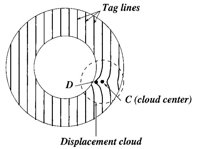
The tag points are displaced around the centre of the cloud given a Gaussian roll-off.

We generated one cloud displacement for each point of the midwall mesh, for each of the local radial, circumferential and longitudinal directions and for a sequence of cloud widths (from 4 to 20 mm, every mm). For each cloud deformation, we compute a displacement field and compute the directional response of the reconstructed field f: knowing the centre of the cloud C, the amplitude CD = ||CD|| and the direction d of the displacement, we define the directional response as:

$$r=\frac{CD-\langle C\mathit{f}\left(C\right)\mid d\rangle }{CD}$$ (12)

where 〈. | .〉 is the 3D scalar product.

Let us examine what a typical behaviour of the displacement response will be with respect to the cloud spatial ‘frequency’ (1/width):

• For an extreme situation where the cloud frequency is zero (which means a cloud of infinite spread and no roll-off), the displacement is a pure translation in the direction CD. All methods can perfectly retrieve translational motion and the ratio is 100%.

• Conversely, for a very high (infinite) cloud frequency (which means a single point displacement), only one point has a significant displacement and the other points do not move. The displacement of the centre of the cloud will be practically ignored when computing the motion, the ratio tends to zero.

Using similar arguments, we can reasonably assume that the response r is a decreasing function with the cloud ‘frequency’ (1/width). The spatial resolution can be defined as the width corresponding to a response of 50%.

3.4. Round robin test on normal heart

In this series of experiments, we tested the methods against one another, in order to cross-validate the techniques. For each method, the displacement field is computed on the golden dataset and new noise-free tag point are generated from the reconstructed motion. The displacement field which is obtained is as close the method can get to a real LV motion. It is actually a good way to build a synthetic model, and the reconstructed motion is actually much more sophisticated (and realistic) than the models found in the literature.

Once the artificial tag points are computed, the other three methods use those ‘simulated’ points to compute the displacement field. The RMS error in residual distances between tag points and deformed tag planes is computed for each method and for each set of generated points. We also computed in the same way RMS error on Lagrangian strains E.

This produces a matrix in which the first entry is the method which generated the points files and second entry is the method which computed the displacement field. The value is the RMS error at end-systole, when the deformation is greatest.

The RMS error which is computed is a classical measure of the standard deviation of the tag distance distribution. It has to be noticed that the standard deviation is not computed on a purely Gaussian random variable: on the contrary, the distance between simulated and data tag points is significantly correlated in space, due to the intrinsic smoothness of (a) the computed displacement field and (b) the tag data which are detected using the FindTags package, even after manual correction. The gradient of the residual between two neighbouring tag points will therefore be small. Moreover, the method used to compute the displacement field forces the displacement field to be continuous and continuously differentiable, inducing smooth variation of the displacement field in space. Therefore, the derivatives of the displacement field (from which strain is defined) also vary smoothly over space and the RMS error is also expected to be small. If there was no smoothing, the computation of the strain would be highly affected by the rapidly varying displacement field and its value would not make any physical sense.

3.5. Pathology database

These experiments are designed to evaluate the relative response of each method with respect to a particular type of motion. We compute a displacement field with each method on a database of LV data containing:

• five normal humans LVs;

• five infarcted human LVs (with at least 70% LAD and/or RCA occlusion as determined by x-ray angiogram);

• four dilated cardiomyopathy human LVs;

• five normal canine LVs injected with dobutamine (10 μg kg^-1 min^-1;

• five right atrial paced canine LVs;

• five right ventricular paced canine LVs (the same subjects as the right atrial paced).

For each method and each patient, we compute the displacement field and the RMS distance error between tag points and the simulated tag points defined as for the round robin section (deformed tag planes intersected with the image planes). Only results at end systole are displayed, for clarity.

Six graphs are drawn showing RMS distance versus subject for each kind of motion. We assume that the database we have collected covers a wide range of possible LV motions.

4. Results

4.1. Strain maps on a normal heart

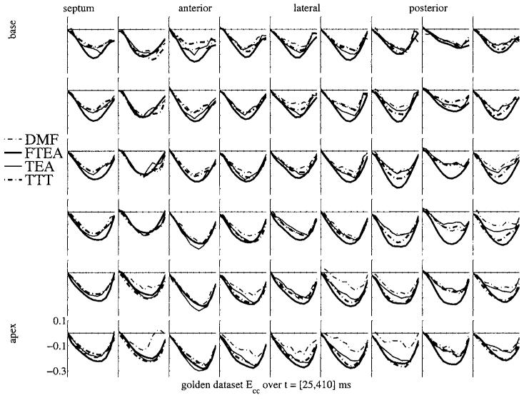
Figure 4 shows the strain map of the golden dataset computed with the four different methods. All strain maps are plotted on top of each other in order to show the consistency or the differences in the strain values. Each box represents the evolution over time of the strain, starting at end-diastole, covering systole and ending after the rapid filling of diastole. The positions of the boxes represent a map of the myocardial mid-wall, from top to bottom, going from base to apex and from left to right, going around the septal, anterior, lateral and then posterior walls.

Figure 4.

Circumferential shortening (E_cc) strain map for the golden dataset for the four methods. Each box shows the strain E_cc as a function of time over systole and early diastole. Thick lines are the 4D methods (FTEA and TTT), thin lines are the 3D methods (DMF and TEA). Broken lines represent the Cartesian methods (DMF and TTT), and full lines represent the ‘polar’ methods (TEA and FTEA).

A first observation of this plot shows that the methods are globally consistent: the trends of the strain evolution are very similar, even during the rapid filling at early diastole (covered by only two time frames). As an example, strain values can be used to define end systole. For each point of the mesh, the strain value E_cc is minimal at a particular time. This time defines the end of contraction (‘local end systole’) for the piece of tissue around this point. For each point of the mesh, the four reconstruction methods give different times of end systole. Computing the standard deviation at each point of the mesh gives a spatial distribution of the dispersion over the different methods of the definition of the ‘local end systole’. Over the mesh, the dispersion of the estimation of local end systole is 32 ms ± 24 ms (mean and standard deviation of the dispersions): these values sit just under the time resolution, showing that, locally, the four methods find with great consistency the same feature in the evolution of the strain value.

Some more accurate observations point out some noticeable differences:

• The apical values are the least coherent, principally due to the difficulty of defining radial, circumferential and longitudinal coordinates in this area.

• The strain curves computed from the 4D methods (TTT and FTEA) are significantly smoother than the ones computed from DMF and TEA which do not perform time interpolation.

• In the posterior wall, the strain values are obviously different, especially for FTEA which significantly overestimate the magnitude of the strain, whereas the other three show more consistency on lower magnitude values.

• The DMF strains are generally lower in magnitude than the TEA and TTT strains, which are themselves lower in magnitude than the FTEA strains. TEA and TTT curves are very similar. The FTEA strains are sometimes significantly larger in magnitude than the other three methods, as in the mid column in the posterior wall.

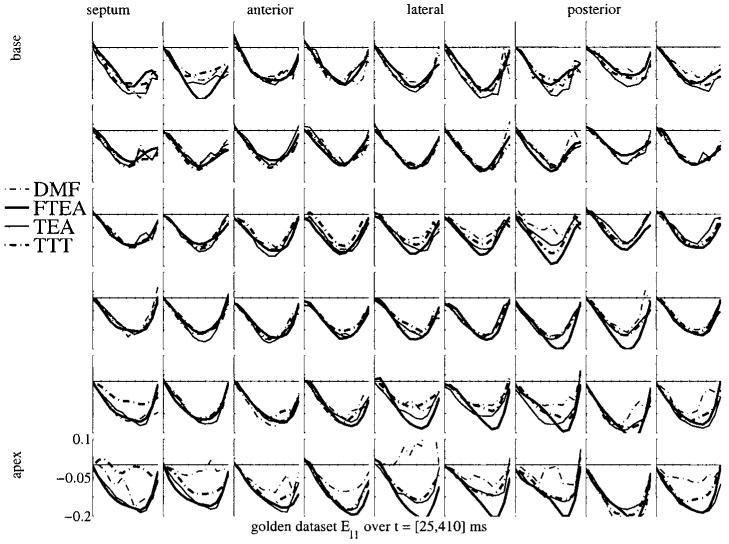
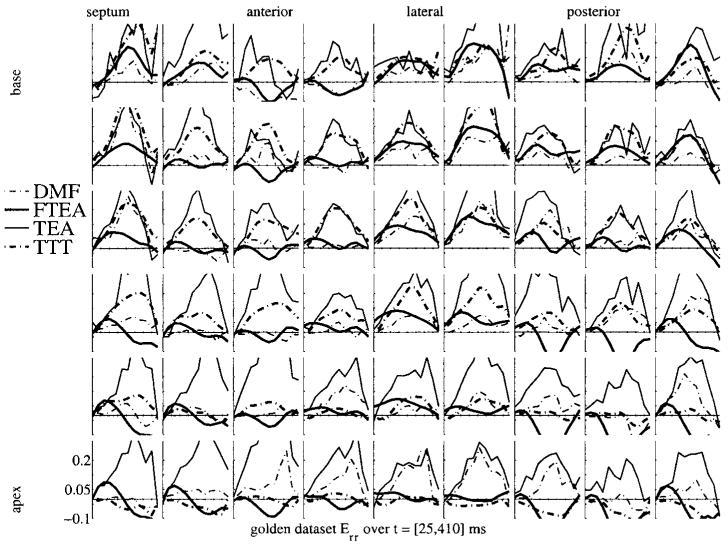
• Figures 5 and 6 show a similar display of strain curves for E_rr and E_ll. The variability in E_ll is even lower than in E_cc, which is expected knowing that the motion in the longitudinal direction is less complex by far than the motion in the short-axis plane. On the contrary, the variability in E_rr is huge. There is no real trend evident in these plots, the local wall thickening is estimated with a very high variability from one method to another. The probable reason for this is the low sampling of the myocardium in the radial direction. Considering a 10 mm thick myocardium and a typical tag spacing of 8 mm, there is only one (maybe two) tag plane(s) which lies in the myocardium. This is obviously not enough to get a reliable estimate of the strain, which, as any derivative, is defined using at least two samples of the displacement in the considered direction. Therefore, the E_rr strain values are strongly influenced (a) by the other directions and (b) by the intrinsic properties of the model which is used to approximate the displacement field. Conversely, this variability in E_rr may explain the variability on E_cc too.

Figure 5.

E_ll strain map for the golden dataset for the four methods. The display is similar to that in figure 4.

Figure 6.

E_rr strain map for the golden dataset for the four methods. The display is similar to that in figure 4.

Considering all these points, it is now clear that there is a need to compare in a more quantitative way the four methods we use. This is the purpose of the experiments described in the following sections.

4.2. Noise immunity

Figure 7 shows the RMS error on Lagrangian strain E in local radial, circumferential, longitudinal (RCL) coordinates at different input noise levels.

Figure 7.

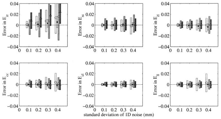
Noise immunity test: for different noise amplitudes, the mean and standard deviation on error on Lagrangian strain E in a local coordinate system (radial, circumferential or longitudinal). The centre of the bar is on the mean value and marked with a sign (○ = DMF, * = FTEA, □ = TEA, △ = TTT), the bar extends up to one standard deviation above and below the mean (from lighter to darker boxes, DMF, FTEA, TEA and TTT).

All errors were below 0.02 for a strain value around -0.3 at end systole for these data. Only E_rr shows a significant important bias and a high sensitivity. This can be due to two reasons:

1. The Lagrangian strain tensor is intrinsically biased when some noise is added to the data (Denney and McVeigh 1997).

2. The displacement in the r direction is the one for which there are fewer data, because there is only one tag line (or two at most) which crosses the myocardium (they are spaced every 8 mm for a wall thickness of approximately 10 mm). This low definition naturally increases the sensitivity to noise.

In this experiment, FTEA is the least sensitive to noise of the four methods in all six strains. DMF, TEA and TTT show similar sensitivities to noise for all strains except in E_cc and E_ll, for which they show more sensitivity. The sensitivity is within acceptable limits for all strain components (the error value is below 10% of the average value of the strain at end systole), except for E_rr.

4.3. Spatial resolution

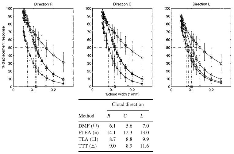
Figure 8 shows the percent of displacement response for different cloud widths and for the radial, circumferential and longitudinal directions. As expected, the greater the width, the higher the response. As a threshold, the width for which the response is 50% is around 6 mm for DMF, whereas it is 9 mm for TEA and TTT and 12 mm for FTEA. All these values are close to the intrinsic resolution of the tagged MR images, which is defined by the tag spacing (between 8 and 10 mm).

Figure 8.

Spatial resolution for each displacement direction (radial, circumferential or longitudinal): top, for different colud widths, the per cent of displacement response for each method (○ = DMF, * = FTEA, □ = TEA, △ = TTT). Bottom, the corresponding values for response of 50%.

4.4. Round robin test on normal heart

The results of RMS error on distance and strain are represented in tables 2 and 3 respectively. In each row is the name of the method which is used to generate artificial tag data. In each column is the name of the method which is used to compute the motion from these data.

Table 2.

The methods in each row i are used to generate artificial tag data T_i. The method in each column j is used to compute the motion from T_i. The figures represent the standard deviation of the RMS error on the distance between (a) the tag points data T_i , and (b) the tag points simulated with the method M_j.

Method used to generate the points	Method used for the fit
	DMF	FTEA	TEA	TTT
DMF	0.18	0.47	0.25	0.35
FTEA	0.21	0.15	0.14	0.27
TEA	0.23	0.47	0.13	0.37
TTT	0.22	0.42	0.22	0.16

Table 3.

As in table 2, the figures represent the RMS error in strain from the motion computed with method M_j on tag data T_i. The values have to be compared with the maximum absolute value of strain E_cc, which is 0.3: all of these RMS errors stay below 10% of the maximal strain value.

Method used to generate the points	Method used for the fit
	DMF	FTEA	TEA	TTT
DMF	0.015	0.018	0.013	0.022
FTEA	0.027	0.011	0.026	0.021
TEA	0.021	0.004	0.023	0.016
TTT	0.024	0.013	0.015	0.016

The RMS error on tag distance shows values which are less than 0.5 mm (one-third of a pixel). The data here are not corrupted by any noise because the tag points have been artificially generated from a smooth deformation field. Therefore, the location of tag points, material points and the values of the strain are precisely known. The error here comes from mainly three sources:

1. The intrinsic inaccuracy of the description of a smooth continuous displacement field with a discretely (and sparsely) sampled set of points. Moreover, the tag points describe only partial information of the motion of the material points.

2. Round off errors and mathematical approximations during the complex processes of matrix inversions which are performed in all methods. Due to the partial condition of the motion written from tag point displacement, these matrices are usually badly conditioned. For FTEA, for instance, the computation of the ${\mathit{f}}_n^{\text{back}}$ directly in 3D generates matrices of size 500 × 500, the computation of f directly in 4D generates a matrix up to 2500 × 2500.

3. The relative differences of the motion models. Of course, a 4D B-spline (like TTT) can only approximate a sequence of prolate spheroidal harmonic development (like on TEA) up to a certain precision.

The off-diagonal elements are a combination of all these three reasons, whereas the diagonal elements of the error matrix are a combination of the first two items:

• The relatively low values of these diagonal terms show the good behaviour of all these methods and ‘auto-validate’ the concept of reconstruction process. (For further development of this validation see Öztürk and McVeigh (1999b).)

• The low values of the off-diagonal terms show that all methods are consistent with one another, each being able to reconstruct within a decent precision the motion another can generate. Table 3 confirms this statement, showing the RMS error on strain in the midwall, comparing the strain computed with one method with the target value computed with the method used to generate the simulated tag data.

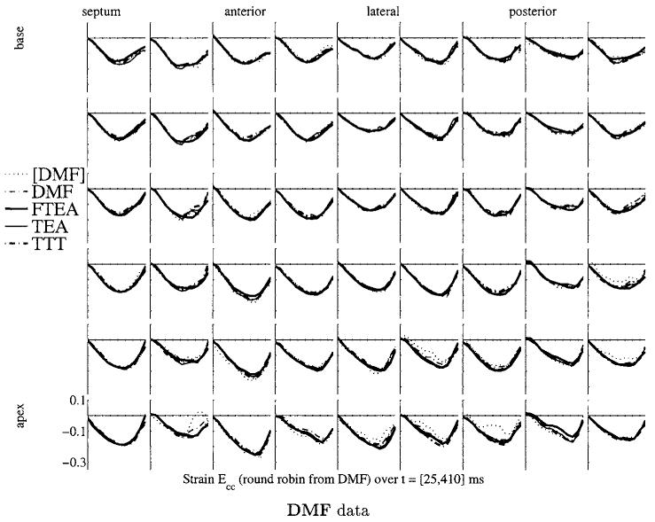
The two tables cross-validate the four methods. Figure 9 also illustrates this result showing the strain map as drawn in figure 4 for the four simulated datasets of the round robin experiment. The curves are much closer to one another than for the golden dataset. Strain maps plotted for E_ll and E_rr show a similar behaviour, even if for the latter the concordance was not as striking. As these strain maps do not provide more significant information than the ones plotted for E_cc, we do not include these in this paper.

Figure 9.

E_cc strain maps for the four methods on the datasets generated for the round robin set of experiments for DMF data. The strain map representation is similar to the one of figure 4.

Figure 9 shows the strain map computed with the four methods from the data generated from DMF. The other maps generated with the other three datasets did not show anything different from what we want to point out: we choose DMF as it is the method which is most sensitive to noise and which has least spatial resolution. The strain curves in figure 4 are the most spiky and irregular, therefore the most challenging to compute for the other three stiffer methods.

The strain maps are much more consistent on this simulated dataset than on the golden dataset. This shows that each method is able to retrieve each other’s motion field with great precision, but none of them actually agrees when the motion is reconstructed from real data. Therefore, in all cases, the modelling of the motion is incorrect (or, to be less dramatic, ‘insufficient’).

As all methods pass the test successfully, the round robin experiment run with DMF, TEA, TTT and FTEA is not discriminating enough. This is mainly because the tagging process sparsely samples the real complex motion of the heart and all the methods use some type of smoothing which is slightly inadequate in all cases: the simulated motion does not reveal all the complexity of the real motion. This shows the limits of this cross-validation approach. However, it has to be noticed that these conclusions are drawn on only one dataset.

4.5. Pathology database

Figure 10 shows the RMS error between real and simulated tag points on the six groups of subjects. This experiment shows a general homogeneity of the results for all methods, for all subjects.

Figure 10.

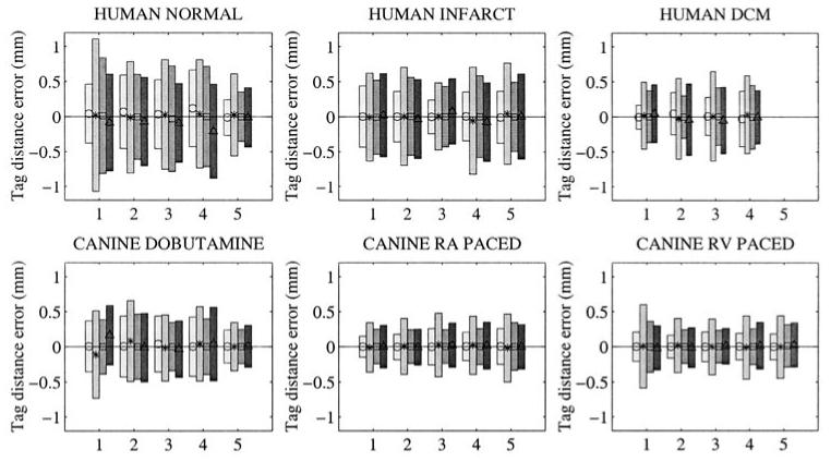
Pathology database: for different types of motion (human normal, infarcted or dilated cardiomyopathy, canine dobutamine, RA or RV paced), the RMS on error on tag distances. Each set of error bars represents one patient (numbered from 1 to 5). For each patient, four error bars are displayed, one for each method (from lighter to darker boxes, ○ = DMF, * = FTEA, □ = TEA, △ = TTT.

The amplitude of the error is higher for normal and infarcted human data than for DCM human and canine data, because the strains in these hearts are greater. The fifth normal dataset is the golden dataset, for which tag points have been segmented more carefully than the other normal hearts, making the distance between simulated and real tag points significantly lower.

The mean error is generally around zero, showing that the estimation of the motion is not biased, except for normal human hearts with the motion computed with TTT. This bias is probably due to the a posteriori 4D approximation done on the control points, whereas DMF and TEA do not perform time smoothing and FTEA computes directly the transformation in 4D.

FTEA gives systematically higher errors and DMF lower results than TEA and TTT, this result follows the trend shown from the cloud experiment. Examining the strain values showed that FTEA was in the majority of the cases overestimating the circumferential strain E_cc, as noticed for the golden dataset. It is interesting to notice that this overestimation could not have been discovered without the quantitative comparisons that have been performed in the round robin test. Further investigations will be performed in order to correct this problem on FTEA.

In any case, none of the methods appear to perform better than the others for one type of motion and worse than the other methods for another type of motion: the order of performance stays consistent.

5. Conclusion

We have presented a series of experiments which compare different methods for reconstructing LV motion from tagged MRI with quantitative measures of performance.

The fits to the golden dataset showed that the methods yield noticeable differences in the displacement and strain, even if the general trends of the motion are apparently correctly detected. The round robin tests showed that there is no obvious source for these differences in the ability of the methods to track data: all methods were able to track output from the other methods, and with much better consistency than from the golden dataset.

There was a consistent trend in the trade-off between spatial resolution and noise immunity. At one end, DMF uses the least amount of smoothing and, as a result, the spatial resolution is highest, but it is the most noise sensitive. At the other end, FTEA uses more smoothing than the other three and is the least noise sensitive, but it has the lowest spatial resolution. TEA and TTT fall somewhere in the middle. DMF tends to slightly underestimate the E_cc strain compared with the strains computed from TEA or TTT, whereas FTEA significantly overestimates it. These results prompted a closer inspection of the FTEA generated displacements; they were found not to deform enough at the endocardial surface due to an insufficient ability to ‘bend’. This method will be tuned such that its noise immunity will suffer, but its ability to bend will increase.

All methods in their current state produced strain maps that were useful for characterizing myocardial function with high precision. The choice of method will depend on the purpose of the user: does one need smooth curves which have lower spatial resolution, or, can one tolerate a higher noise level for better spatial resolution?

The pathology database experiment shows that none of the methods fails for a particular type of motion. If one of the methods had failed, then that method should be simply rejected or at least carefully reviewed. The fact that none of the methods was found to be preferable to the others is desirable, since for a given study, the exact pathology may not be known beforehand or there may be multiple pathologies.

The experiments presented in this paper are fully reproducible to any researchers who would like to perform these tests in order to compare their reconstruction method with these four.

References

- Amini A, Curwen R, Constable RT, Gore JC. 1994 MR physics-based snake tracking and dense deformation from tagged cardiac images; AAAI Symposium on Applications of Computer Vision in Medical Image Processing; Stanford, CA, USA. 1994; Mar 21-23, ( http://noodle.med.yale.edu/alums/amini/aaai_tag/aaai_tag.html) [Google Scholar]
- Arts T, Hunter WC, Douglas A, Muijtjens AM, Reneman RS. Description of the deformation of the left ventricle by a kinematic model. J. Biomech. 1992;25:1119–27. doi: 10.1016/0021-9290(92)90068-c. [DOI] [PubMed] [Google Scholar]
- Atalar E, McVeigh E. Optimization of tag thickness for measuring position with magnetic resonance imaging. Johns Hopkins University School of Medicine; 1994. Technical Report
- Axel L, Dougherty L. MR imaging of motion with spatial modulation of magnetization. Radiology. 1989;171:841–5. doi: 10.1148/radiology.171.3.2717762. [DOI] [PubMed] [Google Scholar]
- Croisille P, Moore CC, Judd RM, Lima JA, Arai M, McVeigh ER, Becker LC, Zerhouni EA. Differentiation of viable and nonviable myocardium by the use of three-dimensional tagged MRI in 2-day-old reperfused canine infarcts. Circulation. 1999;99:284–91. doi: 10.1161/01.cir.99.2.284. [DOI] [PubMed] [Google Scholar]
- Declerck J.Étude de la dynamique cardiaque par analyse d’images tridimensionnelles PhD Thesis 1997Université Nice-Sophia Antipolis [Google Scholar]
- Declerck J, Ayache N, McVeigh ER. Use of a 4D planispheric transformation for the tracking and the analysis of LV motion with tagged MR images. Proc. SPIE. 1999;3660:69–80. [Google Scholar]
- —Research Report 1998a. INRIA RR 3535 http://www.inria.fr/rapports/sophia/RR-3535.html (submitted to IEEE Trans. Med. Imaging)
- Declerck J, Feldmar J, Ayache N. Definition of a four-dimensional continuous planispheric transformation for the tracking and the analysis of left-ventricle motion. Med. Image Anal. 1998b;2:197–213. doi: 10.1016/s1361-8415(98)80011-x. [DOI] [PubMed] [Google Scholar]
- Declerck J, Feldmar J, Goris ML, Betting F. Automatic registration and alignment on a template of cardiac stress and rest reoriented SPECT images. IEEE Trans. Med. Imaging. 1997;16:727–37. doi: 10.1109/42.650870. http://www.inria.fr/rapports/sophia/RR-2270.html [DOI] [PubMed] [Google Scholar]
- Declerck J, Subsol G, Thirion J-P, Ayache N. Computer Vision, Virtual Reality and Robotics in Medicine (Lecture Notes in Computer Science 905) Springer; Berlin: 1995. Automatic retrieval of anatomical structures in 3D medical images; pp. 153–62. (see also INRIA Research Report 2485)
- Denney TS. Estimation and detection of myocardial tags in MR images without user-defined myocardial contours. IEEE Trans. Med. Imaging. 1999;18:330–44. doi: 10.1109/42.768842. [DOI] [PubMed] [Google Scholar]
- Denney TS, McVeigh ER. Model-free reconstruction of three-dimensional myocardial strain from planar tagged MR images. J. Magn. Reson. Imaging. 1997;7:799–810. doi: 10.1002/jmri.1880070506. [DOI] [PMC free article] [PubMed] [Google Scholar]
- Denney TS, Prince JL. Reconstruction of 3D left ventricular motion from planar tagged cardiac MR images: an estimation theoretic approach. IEEE Trans. Med. Imaging. 1995;14:625–35. doi: 10.1109/42.476104. [DOI] [PubMed] [Google Scholar]
- Farin G. Curves and Surfaces for Computer Aided Geometric Design. Academic; New York: 1989. [Google Scholar]
- Fischer SE, McKinnon G, Maier SE, Boesiger P. Improved myocardial tagging contrast. Magn. Reson. Med. 1994;30:191–200. doi: 10.1002/mrm.1910300207. [DOI] [PubMed] [Google Scholar]
- Guttman MA, Prince JL, McVeigh ER. Tag and contour detection in tagged MR images of the left ventricle. IEEE Trans. Med. Imaging. 1994;13:74–88. doi: 10.1109/42.276146. [DOI] [PubMed] [Google Scholar]
- Guttman M, Zerhouni E, McVeigh E. Analysis of cardiac function from MR images. IEEE Comput. Graphics Appl. 1997;17:30–8. doi: 10.1109/38.576854. [DOI] [PMC free article] [PubMed] [Google Scholar]
- Huang T, Amini AA. Volumetric motion tracking of left-ventricle of the heart from tagged MRI by a B-spline solid model. Proc. SPIE. 1999;3660:57–68. [Google Scholar]
- Kraitchman D, Young A, Chang CN, Axel L. Semi-automatic tracking of myocardial motion in MR tagged images. IEEE Trans. Med. Imaging. 1995;14:422–33. doi: 10.1109/42.414606. [DOI] [PubMed] [Google Scholar]
- Kumar S, Goldgof D. Automatic tracking of SPAMM grid and the estimation of deformation parameters from cardiac MR images. IEEE Trans. Med. Imaging. 1994:122–32. doi: 10.1109/42.276150. [DOI] [PubMed] [Google Scholar]
- McVeigh E. Regional myocardial function. Cardiol. Clin. 1998;16:189–206. doi: 10.1016/s0733-8651(05)70008-4. [DOI] [PubMed] [Google Scholar]
- McVeigh E, Atalar E. Cardiac tagging with breath-hold CINE MRI. Magn. Reson. Med. 1992;28:318–27. doi: 10.1002/mrm.1910280214. [DOI] [PMC free article] [PubMed] [Google Scholar]
- Moore CC, McVeigh ER, Zerhouni EA. Non-invasive measurement of three dimensional myocardial deformation with MRI tagging during graded local ischemia. J. Soc. Card. Magn. Reson. 1999;1:207–22. doi: 10.3109/10976649909088333. [DOI] [PMC free article] [PubMed] [Google Scholar]
- Moore CC, Reeder SB, McVeigh ER. Tagged MR imaging in a deforming phantom: photographic validation. Radiology. 1994;190:765–9. doi: 10.1148/radiology.190.3.8115625. [DOI] [PMC free article] [PubMed] [Google Scholar]
- Mosher TJ, Smith TB. A DANTE tagging sequence for the evaluation of translational sample motion. Magn. Reson. Med. 1990;15:334–9. doi: 10.1002/mrm.1910150215. [DOI] [PubMed] [Google Scholar]
- Moulton MJ, Creswell L, Downing S, Actis R, Szabo B, Vannier M, Pasque M. Spline surface interpolation for calculating 3D ventricular strains from MRI tissue tagging. Am. J. Physiol. 1996;270:H281–H297. doi: 10.1152/ajpheart.1996.270.1.H281. [DOI] [PubMed] [Google Scholar]
- O’Dell WG, Moore CC, McVeigh ER. Three-dimensional myocardial deformations: calculation with displacement field fitting to tagged MR images. Radiology. 1995;195:829–35. doi: 10.1148/radiology.195.3.7754016. [DOI] [PMC free article] [PubMed] [Google Scholar]
- O’Donnell T, Boult T, Gupta A. Global models with parametric offsets as applied to cardiac motion recovery. IEEE Comput. Vision Pattern Recognition. 1996:293–9. [Google Scholar]
- Öztürk C, McVeigh ER. Four-dimensional B-spline based motion analysis of tagged cardiac MR images. Proc. SPIE. 1999a;3660:46–56. [Google Scholar]
- — . ISMRM’99. 1999b. In-vivo validation of 4D B-spline-based motion tracking algorithm for cardiac tagged MRI; p. 1284. [Google Scholar]
- Park J, Metaxas D, Axel L. Analysis of left ventricular motion based on volumetric deformable models and MRI-SPAMM. Med. Image Anal. 1996;1:53–71. doi: 10.1016/s1361-8415(01)80005-0. [DOI] [PubMed] [Google Scholar]
- Press WH, Flannery BP, Teukolsky SA, Vetterling WT. Numerical Recipes in C, the Art of Scientific Computing. Cambridge University Press; Cambridge: 1992. [Google Scholar]
- Radeva P, Amini A, Huang J. Deformable B-solids and implicit snakes for localization and tracking of MRI-SPAMM data. Comput. Vision Image Understanding. 1997;66:163–78. [Google Scholar]
- Waks E, Prince J, Douglas A. Cardiac motion simulator for tagged MRI. Math. Methods Biomed. Image Anal. 1996:182–91. [Google Scholar]
- Young AA. Medical Image Computing and Computer-Assisted Intervention—MICCAI (Lecture Notes in Computer Science. Vol. 1496. Springer; Berlin: 1998. Model tags: direct 3D tracking of heart wall motion from tagged MR images; pp. 92–101. [Google Scholar]
- Young AA, Axel L. Three-dimensional motion and deformation of the heart wall: estimation with spatial modulation of magnetization—a model-based approach. Radiology. 1992;185:241–7. doi: 10.1148/radiology.185.1.1523316. [DOI] [PubMed] [Google Scholar]
- Young A, Kraitchman D, Dougherty L, Axel L. Tracking and finite element analysis of stripe deformation in magnetic resonance tagging. IEEE Trans. Med. Imaging. 1995;14:413–21. doi: 10.1109/42.414605. [DOI] [PubMed] [Google Scholar]
- Zerhouni E, Parish D, Rogers W, Yang A, Shapiro E. Human heart: tagging with MR imaging—a method for non-invasive assessment of myocardial motion. Radiology. 1988;169:59–63. doi: 10.1148/radiology.169.1.3420283. [DOI] [PubMed] [Google Scholar]