In Vivo Measurement of $T_2^{\ast }$ and Field Inhomogeneity Maps in the Human Heart at 1.5 T

Abstract

Cardiac echo-planar imaging suffers invariably from regions of severe distortion and $T_2^{\ast }$ decay in the myocardium. The purpose of this work was to perform local measurements of $T_2^{\ast }$ and field inhomogeneities in the myocardium and to identify the sources of focal signal loss and distortion. Field inhomogeneity maps and $T_2^{\ast }$ were measured in five normal volunteers in short-axis slices spanning from base to apex. It was found that $T_2^{\ast }$ ranged from 26 ms (SD = 7 ms, n = 5) to 41 ms (SD = 11 ms, n = 5) over most of the heart, and peak-to-peak field inhomogeneity differences were 71 Hz (SD = 14 Hz, n = 5). In all hearts, regions of severe signal loss were consistently adjacent to the posterior vein of the left ventricle; $T_2^{\ast }$ in these regions was 12 ms (SD = 2 ms, n = 5), and the difference in resonance frequency with the surrounding myocardium was 70-100 Hz. These effects may be caused by increased magnetic susceptibility from deoxygenated blood in these veins.

INTRODUCTION

The rapid imaging times of echo-planar imaging (EPI) are ideally suited for cardiac imaging (1,2). EPI has excellent SNR behavior and has been applied to applications such as bolus tracking of contrast agents for evaluation of cardiac perfusion studies (3-6) as well as myocardial blood oxygenation level dependent imaging (7-14). Furthermore, EPI provides superior tag-tissue contrast over standard gradient-echo imaging for motion studies involving cardiac tagging (15).

EPI is inherently $T_2^{\ast }$ weighted and sensitive to field inhomogeneities, suffering from significant signal loss and distortion in focal regions of the myocardium. Four short-axis cardiac gradient echo-planar images are shown in Fig. 1. As the duration of the echo train increases, a signal void in the posterior-lateral region of the heart becomes more prominent (arrows), caused by very rapid $T_2^{\ast }$ decay. Increasing the echo train length further degrades image quality because of increased distortion, caused by severe field inhomogeneities commonly experienced in the vicinity of the heart.

FIG. 1.

Short-axis gradient-echo planar images of the heart acquired in basal, midventricular, and apical slices at ±64 kHz, 128 × 128 matrix, FOV = 24 cm. Spatial-spectral excitation was used to eliminate fat signal. For these images, the echo train length and TE were (columns, left to right): 8 echoes, 24 ms; 16 echoes, 29 ms; 32 echoes, 43 ms; 64 echoes, 69 ms. Focal regions of signal loss and distortion are marked with white arrows. The phase-encoding direction is oriented 30° from horizontal, sloping down from left to right.

Cardiac spiral imaging will also be affected by rapid $T_2^{\ast }$ decay, since spiral readouts are approximately 15–20 ms in duration (16). Regions of high field inhomogeneities may also experience blurring since the point spread function of spiral imaging broadens in the presence of off-resonance spins.

Although in vivo measurements of T₂ in the myocardium have been reported (17, 18), relatively few reports of myocardial $T_2^{\ast }$ are available. This may be due, in part, to the fact that $T_2^{\ast }$ is highly dependent on field homogeneity and the orientation of the heart in the magnet, as well as imaging parameters such as slice thickness. Jaffer et al. recently reported $T_2^{\ast }$ to be 20 ms in the anterior wall of the heart, at 4.0 T (19).

Measurements of field maps are largely restricted to automated B_o shimming applications in the brain (20-22), although Jaffer et al. have reported measurements of field inhomogeneities in the vicinity of the heart, at 4.0 T, using chemical shift imaging time averaged over the cardiac cycle (19).

In this work, we measured $T_2^{\ast }$ in normal volunteers (n = 5) at 1.5 T, characterizing $T_2^{\ast }$ in different regions of the heart, as well as identifying the sources of focal $T_2^{\ast }$ decay. In the same volunteers, field maps were measured at different phases through the cardiac cycle.

THEORY

Field Perturbations from Large Epicardial Veins

A short-axis view of the heart and the three major epicardial veins of the left ventricle are schematically diagrammed in Fig. 2. The coronary sinus is not shown because it lies in the coronary sulcus basal to short-axis views of the left ventricle. As will be shown, the location of these vessels correlates closely with regions of severe signal loss in $T_2^{\ast }$-weighted images. In this section, estimates of $T_2^{\ast }$ in the vicinity of large veins are made in an attempt to explain the decreased $T_2^{\ast }$ seen in these regions.

FIG. 2.

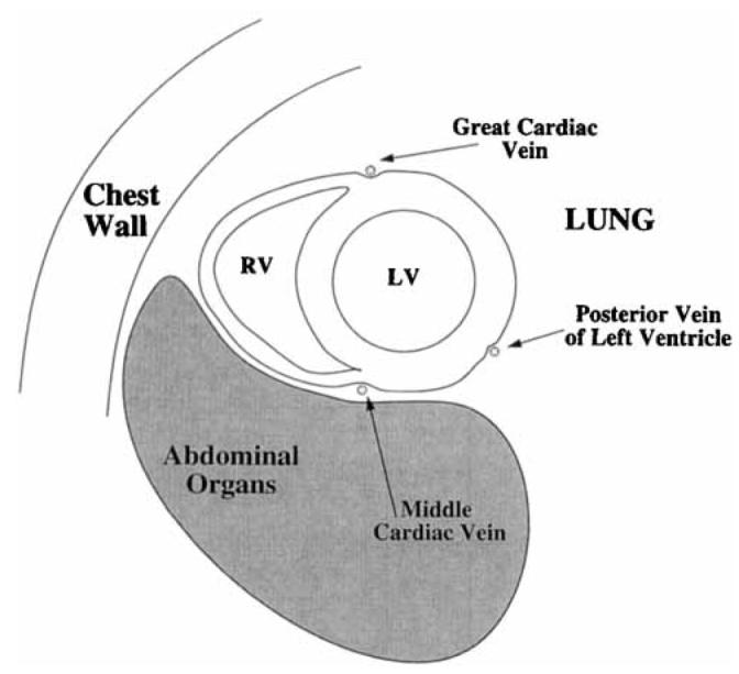
Schematic short-axis view of the heart showing the major epicardial veins of the left ventricle.

Consider the z component of the magnetic field perturbation (cgs units) surrounding the cylindrical vessel shown in Fig. 3 (23-26),

$$\Delta B_{\mathrm{z}}(r,\varphi )=\{\begin{array}{cc}2\pi {\left(\frac{B_c}{r}\right)}^2{B}_0\Delta {\chi }_v\cos 2\varphi {\sin }^2\alpha \hfill & r\ge R_c\hfill \\ \frac{2\pi }{3}{B}_0\Delta {\chi }_v(3{\cos }^2\alpha -1)\hfill & r<R_c\hfill \end{array}\phantom{\}}$$ [1]

where Δχ_v is the susceptibility difference between deoxygenated blood inside the vessel and the surrounding tissue, R_c is the radius of the vessel, B_o is the main magnetic field, and α is the angle between the axis of the vessel and the main magnetic field. This equation describes the magnetic field perturbation in the (u, v, w) coordinate system, where the axis of the vessel is coincident with the v axis. In this frame, the standard cylindrical coordinates are (r, ϕ, v), where ϕ = 0 along the w axis. This modified coordinate system has been chosen so that B_o lies in the z direction.

FIG. 3.

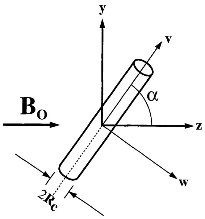
Cylindrical vein at an angle α to the main magnetic field, B_o in the z direction. The axis of the vein is in the y-z plane, and (u, v, w) are the coordinates of the vessel with the axis of the vessel in the v direction. The axis of the vein is in the y-z plane, and (u, v, w) are the coordinates of the vessel with the axis of the vessel in the v direction. The y, z, v and w axes are in the plane of the page, and the u and x axes point into the page.

Enhanced $T_2^{\ast }$ Decay

$T_2^{\ast }$ decay is enhanced by through-slice dephasing of spins caused by the component of the field perturbation gradient oriented in the through-slice direction. The gradient (G/cm) of the z component of the field perturbation outside the vessel is,

$$\begin{array}{cc}\hfill \underset{‒}{G}(r,\varphi )& =\nabla \left(\Delta B_z(r,\varphi )\right)\hfill \\ \hfill & =-\frac{4\pi B_0\Delta {\chi }_v{R}_c^2{\sin }^2\alpha }{r^3}(\widehat{r}\cos 2\varphi +\widehat{\varphi }\sin 2\varphi )\hfill \end{array}$$ [2]

where ▽ is the gradient operator, and r̂ and ϕ̂ are unit vectors that define the cylindrical coordinate system of the vessel. The gradient of the field perturbation inside the vessel is zero. In Cartesian coordinates, Eq. [2] becomes,

$$\underset{‒}{G}(u,v,w)=-\frac{4\pi B_0\Delta {\chi }_v{R}_c^2{\sin }^2\alpha }{{(u^2+w^2)}^{3∕2}}(\widehat{u}\sin 3\varphi +\widehat{w}\cos 3\varphi )$$ [3]

where $\varphi ={\tan }^{-1}\left({}^u∕_w\right)$. Rotation of the coordinate system to obtain the gradient in (x, y, z) coordinates is ascertained by rotation of G(u, v, w),

$$\underset{‒}{G}(x,y,z)=\mathbf{R}\underset{‒}{G}(u,v,w)$$ [4]

where R is the coordinate system rotation matrix required to rotate (u, v, w) coordinates to the (x, y, z) coordinates of the magnet.

Knowing the vector field describing this field gradient in magnet coordinates, one can now determine the total signal from the position (x_s, y_s) in the slice.

$$s(x_s,y_s,t)=\int e^{-[t∕T_2^{\ast }(x_s,y_s,z_s)]}\rho (x_s,y_s,z_s)e^{j\gamma \underset{‒}{G}(x,y,z)\cdot {\widehat{z}}_s{z}_{s}t}{\mathit{dz}}_s$$ [5]

where the integral is evaluated through the slice at position (x_s, y_s), $T_2^{\ast }(x_s,y_s,z_s)$ characterizes the decay of transverse magnetization at position (x_s, y_s, z_s) in the absence of bulk susceptibility effects from the cylindrical vessel, $\underset{-}{G}(x,y,z)\cdot {\widehat{z}}_s$ is the component of the field gradient in the through-slice direction, and t is time. This equation can be solved numerically and the resulting decay can be fit to an exponential to estimate the observed $T_2^{\ast }$ at different positions within the image.

Clearly, estimates of $T_2^{\ast }$ are highly dependent upon the geometry and orientation of the vessel with respect to both B_o and the imaging plane. To make some quantitative estimates of $T_2^{\ast }$ using reasonable parameters, we assume that,

1. The slice is in the y = 0 plane, i.e., ${\widehat{z}}_s=\widehat{y}$, and the slice thickness (Δz_s) is 8 mm.

2. The radius of a large epicardial vein (R_c) is approximately 1 mm.

3. The saturation of the venous coronary blood is approximately 30% (27). At 0% saturation, the susceptibility of blood (HCt = 40%) is 0.08 ppm (28). As described by Kennan et al. (29), the susceptibility of 30% saturated blood would be (1 − 0.3) × 0.08 ppm = 0.056 ppm.

4. $T_2^{\ast }$ in the myocardium is 35 ms, and $T_2^{\ast }$ in the vessel is 12 ms. The latter value was chosen by extrapolating in vivo measurements of $T_2^{\ast }$ in whole blood (30).

With these assumptions, the through-slice field perturbations were calculated, as shown in Fig. 4a. This figure is a field perturbation contour plot, in the x = 0 plane, cutting through both the vessel, oriented at 70°, and the imaging slice, which lies in the y = 0 plane. Significant through-slice variations in the field perturbations are evident. These perturbations will enhance $T_2^{\ast }$ decay, as shown in Fig. 4b, a contour plot of $T_2^{\ast }$ in the vicinity of a 1-mm radius epicardial vein oriented 70° to the magnetic field, with the imaging slice in the y = 0 plane, 30% desaturated blood (HCt = 40%), and a slice thickness of 8 mm.

FIG. 4.

(a) Contour plot of the field perturbations (mG) in the y-z plane, cutting through a 1 -mm radius epicardial vein oriented 70° to the magnetic field. Horizontal lines are the upper and lower boundaries of the 8-mm-thick slice. (b) Contour plot of $T_2^{\ast }$ (ms) in the x-z plane through the vessel. Dashed lines indicate the projection of the intersection of the vessel with the slice boundaries. It has been assumed that the blood is 70% desaturated blood (HCt = 40%) and the inherent $T_2^{\ast }$ of the blood and myocardium is 12 ms and 35 ms, respectively.

For this model, it is interesting to note that no $T_2^{\ast }$ decay enhancement resulting from the field perturbations of the cylinder will occur when the slice is oriented perpendicular to the vessel. This occurs because the field gradient in the through-slice direction is zero, causing no through-plane dephasing of spins. In-plane distortion will still be present, however, and is maximized for this orientation.

Although these estimates of $T_2^{\ast }$ are based on several assumptions, the potential for substantial signal loss in long-TE gradient-echo sequences is apparent.

Distortion From In-Plane Perturbations

Whereas through-plane magnetic field perturbations enhance $T_2^{\ast }$ decay, in-plane perturbations cause image distortion. This distortion is particularly severe in the phase-encoding direction of echo-planar images with long echo trains. The distortion in the phase-encoding direction, at a position (x_s, y_x), has been described previously for multishot EPI (2, 31),

$$\Delta y(x_s,y_s)=\frac{T_{ro}\Delta {\stackrel{‒}{B}}_z(x_s,y_s)}{n_i\Delta G_y\Delta t_y}$$ [6]

where T_ro is the time between echoes in an echo train, n_i is the number of shots, n_iΔG_yΔt_y is the area under each phase-encoding blip, and ΔB̄_z(x_s, y_s) is the average through-plane field perturbation at the position (x_s, y_s).

As an example, we calculated the field inhomogeneity map shown in Fig. 5a near a vessel perpendicular to B₀, using the same assumptions listed in the previous section. The resulting distortion in the phase-encoding direction, calculated from Eq. [6], is depicted in Figs. 5b and 5c for 16-, eight-, and two-shot echo-planar images with T_ro = 1.5 ms, and a 28-cm FOV (γΔG_yΔt_y = 0.22 cm^−l). The signal from material inside the vessel has been ignored in the plots in Figs. 5b and 5c.

FIG. 5.

(a) Contour plot of the field map (mG) in the x-z plane near a 1-mm epicardial vein oriented perpendicular to the B₀ field and the imaging plane. (b) Distortion in the phase-encoding direction resulting from field inhomogeneities shown in (a) for 16 shots, (c) eight shots, and (d) two shots. It has been assumed that the blood is 70% desaturated, T_ro = 1.5 ms, and FOV = 28 cm (γΔG_yΔt_y = 0.22 cm⁻¹).

MATERIALS AND METHODS

All imaging was performed on a GE Signa 1.5-T Horizon (version 5.6, General Electric Medical Systems, Milwaukee, WI). This scanner has shielded gradients with maximum gradient strength of 2.2 G/cm and slew rate of 120 ${}^T∕_{ms}$ on all three axes.

In five male volunteers (age: range 21–37 years, median 31 years, mean 28.6 years), breath-hold, ECG-gated, spoiled gradient-echo images (FOV = 32–36 cm, Δz = 8 mm, α = 15–20°) were acquired in three short-axis slices equally spaced from base to apex. Flow compensation was used for all imaging, and all volunteers lay supine along the bore of the magnet. The body coil was used to transmit RF and a four-coil phased-array unit was used to receive signal for measurement of $T_2^{\ast }$. A single-receiver flexible surface coil was used for field map measurements to avoid issues of combining complex data sets from multiple coils (32).

Measurement of $T_2^{\ast }$ was performed by acquiring images with TR = 50 ms and varying TE from 2.4 to 45 ms to obtain $T_2^{\ast }$ decay curves. Multiple phases (three to five) were acquired during the cardiac cycle with 200-ms time resolution and a matrix size of 256 × 160. Total breath-hold time was 37–42 s (40 heartbeats) for each slice.

Field inhomogeneity maps were acquired using TR = 14 ms and varying TE from 4.4 to 8.8 ms to obtain two-point fits. This choice of TEs ensured that fat and water resonances were in phase, preventing chemical shift from affecting field inhomogeneity maps. Both sets of images were acquired in the same breath-hold to ensure accurate registration of the images acquired at different values of TE. Multiple phases (nine to 13) were acquired over the entire cardiac cycle with 112-ms time resolution and a matrix size of 256 × 128. Total breath-hold duration was 35–40 s, depending on the resting heart rate of the volunteer.

Field maps were calculated on a pixel basis using the phase-difference method (33) to determine the off-resonance frequency at a position (x_s, y_s),

$$\begin{array}{cc}\hfill \Delta f(x_s,y_s)& =\frac{\gamma }{2\pi }\Delta {\stackrel{‒}{B}}_z(x_s,y_s)\hfill \\ \hfill & =\frac{\arg \left(S_2(x_s,y_s)S_1^{\ast }(x_s,y_s)\right)}{2\pi ({\mathrm{TE}}_2-{\mathrm{TE}}_1)}\hfill \end{array}$$ [7]

where S₁(x_s, y_s) and S₂(x_s, y_s), are the complex signals of the two images acquired at TE₁ and TE₂, respectively. Complex conjugation is denoted by an asterisk (*).

RESULTS

$T_2^{\ast }$ Results

$T_2^{\ast }$-weighted images from one volunteer for three slices at five (of nine) TE values are shown in Fig. 6. A clear darkening is seen particularly in regions adjacent to the posterior vein of the left ventricle. As well, in the apical images of two volunteers, a severe darkening is seen adjacent to the interventricular sulcus, where the great cardiac vein lies.

FIG. 6.

Typical short-axis images of a normal volunteer, acquired at increasing values of TE. Severe darkening is seen at longer TEs, as indicated by white arrows. For these images, TR = 50 ms, FOV = 32 cm, Δz_s = 8 mm, and flow compensation was used.

High spatial resolution images (0.7 × 0.9 × 8 mm³ voxel size) were acquired through systole in an apical slice of one volunteer, to visualize the structure associated with the focal signal loss. Figs. 7a through 7c are three time frames of 14 high-resolution images acquired through systole. In Fig. 7a (arrow), a bright vessel can be seen, which exhibits maximum brightness during early systole, indicating maximum flow enhancement. Images in Figs. 7b and 7c were acquired at late systole and early diastole, respectively, when venous coronary flow is very low. This flow pattern is most evident when the images are displayed in a CINE movie through the cardiac cycle and is consistent with the flow patterns expected from an epicardial cardiac vein (34). Figure 7d is a $T_2^{\ast }$-weighted image (TR = 50 ms, TE = 20 ms) showing a region of focal signal loss in the posterior wall (arrow) of the same slice shown in Figs. 7a through 7c. This region lies directly adjacent to the epicardial vein.

FIG. 7.

Short-axis images at (a) early systole, (b) end systole, and (c) late diastole. A large epicardial vein appears bright in early systole when flow is high. The signal from the vessel is not seen during late systole or diastole when flow is close to zero. Image parameters include: TR = 12 ms, TE = 2.2 ms, 0.7 × 0.9 × 8 mm³ voxel size, 48 ms per movie frame, three averages, ±32 kHz. (d) A $T_2^{\ast }$-weighted image of the same slice using the same parameters as the images shown in Fig. 6, with TR = 50 ms and TE = 20 ms.

Regions of severe signal loss adjacent to the posterior vein of the left ventricle were observed in all volunteers. In two volunteers, regions of signal loss adjacent to the great cardiac vein were seen in apical slices. Basal, midventricular, and apical short-axis images from all five volunteers [at TE = 15 ms) are shown in Fig. 8. Regions of signal loss are marked by white arrows. The same region of signal loss adjacent to the posterior vein of the left ventricle is seen in all volunteers. In these images, regions of signal deficit are also seen adjacent to the great cardiac vein in Subjects 4 and 5.

FIG. 8.

Basal, midventricular, and apical short-axis images of all volunteers at TE = 15 ms. Regions of severe darkening are indicated with white arrows.

In Fig. 9, normalized signal intensities from regions of interest (ROIs) in the septum and the area adjacent to the posterior cardiac vein, in one volunteer, are plotted, showing the enhanced decay near the posterior vein of the left ventricle.

FIG. 9.

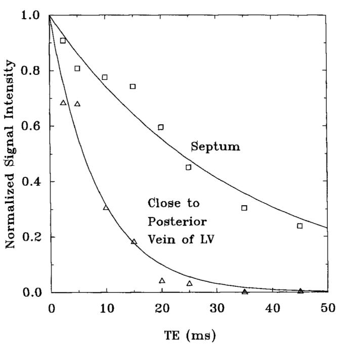
$T_2^{\ast }$ decay curves from the septum and a region adjacent to the posterior vein of the left ventricle in the midventricular slice of one volunteer. The $T_2^{\ast }$ values measured from these curves were 34 ms from the septum and 9 ms from the area adjacent to the posterior vein of the left ventricle.

Summarized in Table 1 are the $T_2^{\ast }$ values averaged over all five volunteers in each of the three short-axis slices. Within each slice, $T_2^{\ast }$ was measured from ROIs in the septum, lateral wall, anterior wall, and posterior wall. As well, $T_2^{\ast }$ was measured in a region adjacent to the posterior cardiac vein to quantify the focal signal loss seen in this region. Lastly, $T_2^{\ast }$ was measured in regions that displayed significant signal loss adjacent to the great cardiac vein.

Table 1.

Summary of the $T_2^{\ast }$ Measured in Basal, Mid, and Apical Short-Axis Slices, from ROls Positioned in the Septum, Posterior Wall, Lateral Wall, and Anterior Wall

	Base	Mid	Apex
Septum	32 ± 5 (n = 5)	38 ± 6 (n = 5)	38 ± 6 (n = 5)
Posterior wall	26 ± 7 (n = 5)	28 ± 3 (n = 5)	34 ± 5 (n = 5)
Lateral wall	36 ± 8 (n = 5)	41 ± 11 (n = 5)	38 ± 7 (n = 5)
Anterior wall	29 ± 9 (n = 5)	31 ± 7 (n = 5)	34 ± 9 (n = 5)
Posterior vein	13 ± 2 (n = 5)	12 ± 3 (n = 5)	12 ± 2 (n = 5)
Great cardiac vein	—	—	8 ± 2 (n = 2)

As well, $T_2^{\ast }$ was measured in regions adjacent to the posterior vein of the left ventricle and the great cardiac vein, which showed focal signal loss.

No significant $T_2^{\ast }$ differences were observed between slices or within a slice for $T_2^{\ast }$ measured in the septal, posterior, lateral, or anterior walls, as calculated by analysis of variance (P > 0.07). Differences between these regions and the area adjacent to the posterior vein of the left ventricle were highly significant, however, as calculated with Scheff6 post-hoc grouping analysis (P < 0.005) (35).

In one volunteer, measurements of $T_2^{\ast }$, were performed at different slice thicknesses (4 mm, 6 mm, 8 mm, and 10 mm) at one location. No differences in $T_2^{\ast }$ were detectable in any region of the heart, as the slice thickness changed.

Field Map Results

Field inhomogeneity maps (Hz) are shown in Fig. 10 for all volunteers in basal, midventricular, and apical slices, at a midsystolic image frame. Focal regions of inhomogeneities are evident, particularly near the posterior vein of the left ventricle; this focal region was seen in every volunteer. Minimal phase wrap was seen over the region of the heart, suggesting that the choice of TE (4.4 and 8.8 ms) did not produce significant frequency ambiguities.

FIG. 10.

Field maps of all five volunteers in basal, rnidventricular, and apical slices. Arrows denote regions of focal inhomogeneity. A scale is shown, mapping signal intensity to off-resonance frequencies.

Strong correlation is seen between the regions of high field inhomogeneities in Fig. 10 and the regions of focal signal decay in Fig. 8.

In two volunteers, additional measurements were made, with the time order of the two TE values reversed, to test whether desaturation of blood during breath-holding would alter the field maps. No detectable differences were seen between field maps acquired with the TE values in the opposite order during the same breath-hold.

The field inhomogeneities averaged over all five volunteers in each of the three short-axis slices are summarized in Table 2. Within each slice, the frequency offset relative to that in the midventricular septum was measured in the anterior wall, lateral wall, and posterior wall. Reference to the midventricular septum eliminated bulk resonance differences between volunteers. Frequency offsets in regions adjacent to the posterior cardiac vein were measured to quantify the large field inhomogeneity seen in this region. Regions in the field map that experienced phase wrapping in regions of focal inhomogeneity were unwrapped to determine the actual off-resonance frequencies.

Table 2.

Summary of the Field lnhomogeneities (Hz) Measured in Basal, Mid, and Apical Short-Axis Slices, from ROls Positioned in the Septum, Posterior Wall, Lateral Wall, and Anterior Wall

	Base	Mid	Apex
Septum	−6 ± 2  (n = 5)	0   (n = 5)	2 ± 15 (n = 5)
Posterior wall	−7 ± 20 (n = 5)	7 ± 10 (n = 5)	4 ± 34 (n = 5)
Lateral wall	20 ± 19 (n = 5)	26 ± 20 (n = 5)	21 ± 12 (n = 5)
Anterior wall	31 ± 16 (n = 5)	37 ± 7  (n = 5)	44 ± 17 (n = 5)
Posterior vein	−65 ± 40 (n = 5)	−70 ± 26 (n = 5)	−65 ± 45 (n = 5)
Great cardiac vein	—	—	113 ± 27 (n = 2)

All measurements are relative to the midventricular septum. Field inhomogeneities were also measured in ROls adjacent to the posterior vein of the left ventricle and the great cardiac vein.

The peak-to-peak off-resonance within each heart was measured (excluding the regions near vessels), and the average peak-to-peak variation was found to be 71 Hz (SD = 14 Hz, n = 5).

No significant differences of the field inhomogeneity maps were observed between slices in the septal, posterior, lateral, or anterior walls. There were significant in-plane differences, however, between the septal-posterior and the anterolateral regions, as calculated with Scheff6 post-hoc grouping analysis (P < 0.02). Differences between these regions and the area adjacent to the posterior vein of the left ventricle were highly significant (P < 0.005). These differences can also be appreciated from the field maps in Fig. 10, In all volunteers, little change in the field map was seen as the heart contracted through systole.

A “streaking” artifact can be appreciated in the apical echo-planar images of Fig. 1 adjacent to the great cardiac vein. The streak is in the phase-encoding direction, which has been rotated 30° clockwise from horizontal. The location of this artifact is denoted with white arrows and correlates very closely with a region of high field inhomogeneity seen in the field map image (Volunteer 4 in Fig. 10). The $T_2^{\ast }$ measured in this region was 8 ms. This artifact is consistent with the distortion predicted by the distortion calculations shown in Fig. 5 for long echo train lengths.

DISCUSSION

In this work, the $T_2^{\ast }$ and field inhomogeneity maps in the hearts of five normal volunteers were measured in apical, midventricular, and basal short-axis slices at 1.5 T. In these slices, the average $T_2^{\ast }$ was found to be approximately 26 ms (SD = 7 ms, n = 5) to 41 ms (SD = 11 ms, n = 5) and the average peak-to-peak field inhomogeneity was 71 Hz (SD = 14 Hz, n = 5).

Focal regions of enhanced $T_2^{\ast }$ decay were seen in areas adjacent to the posterior vein of the left ventricle in all hearts. In two volunteers, a significant region of signal loss was also seen in the area adjacent to the great cardiac vein. The focal nature of these regions strongly suggests the influence of these veins on the observed $T_2^{\ast }$, measured to be 12 ms adjacent to the posterior vein of the left ventricle and 8 ms adjacent to the great cardiac vein.

Although the region of myocardium adjacent to the posterior vein of the left ventricle consistently experienced enhanced $T_2^{\ast }$ decay, regions adjacent to the middle coronary vein did not. This large vein lies in the posterior interventricular sulcus and sits immediately superior to the diaphragm and liver. A compensatory effect from the liver or a different orientation with respect to the imaging slice or main magnetic field may explain the lack of focal signal loss from this vessel.

Measurement of $T_2^{\ast }$ will depend on several imaging parameters, most notably the slice thickness, since through-plane dephasing of spins is responsible for enhanced $T_2^{\ast }$ decay. For linear inhomogeneities, it is well known that decreasing slice thickness will reduce through-plane dephasing, increasing $T_2^{\ast }$. Focal inhomogeneities, however, have complex geometrical dependencies and the effect of slice thickness on the observed $T_2^{\ast }$ is not obvious. In one volunteer, no changes in $T_2^{\ast }$ were observed as slice thickness was increased from 2 to 10 mm.

An analytical description of the $T_2^{\ast }$ behavior in the vicinity of a cylindrical vessel was also presented in an attempt to estimate $T_2^{\ast }$ in regions adjacent to coronary veins. Measurements of $T_2^{\ast }$ in the region adjacent to the posterior vein of the left ventricle agree closely with that predicted with the numerical analysis. A large proportion of the decreased $T_2^{\ast }$ results from the low $T_2^{\ast }$ of the blood itself. The increased spatial extent of this decay, however, results from the inhomogeneous magnetic field created by susceptibility differences between the vessel and the myocardium. Although this analysis is highly orientation dependent, attempts were made to use parameters close to those encountered with typical in vivo human cardiac studies.

In gradient-echo images, distortion cannot explain the focal signal loss with progressive increases in TE, since there is no distortion in the phase-encoding direction and the distortion in the readout direction is constant. For EPI images with long echo train lengths, however, the field inhomogeneities in these regions will cause significant image distortion in the phase-encoding direction. Computation of the distortion in echo-planar images in the vicinity of vessels carrying deoxygenated blood were performed, and the results of these calculations predict a streaking artifact in the phase-encoding direction, per Eq. [6]. This distortion is evident in Fig. 1, particularly in the lateral wall and adjacent to the posterior vein of the left ventricle.

The $T_2^{\ast }$ of blood in the coronary veins is dependent on the oxygen desaturation of that blood. Venous desaturation resulting from extended breath-holds would have contributed little to the desaturation of blood in the coronary veins, since arterial coronary oxygen extraction fractions are large in the myocardium, leaving venous blood largely desaturated, even at rest. This implies that long breath-holds should have had little impact on the desaturation of the venous blood, and thus on the measured $T_2^{\ast }$. Stehling et al. measured arterial hemoglobin desaturation and changes in cerebral signal intensity during apnea and found that approximately 2 min were required before changes in signal intensity were detectable (36). As well, no changes of the field maps were seen when the order of the two images acquired during a breath-hold (each with different TE values) was reversed.

Field inhomogeneity maps were also measured in the same five volunteers, at the same positions in the heart. Except in areas adjacent to vessels, the field inhomogeneities varied smoothly over the heart. A significant difference of the off-resonance frequencies between the septal-posterior and anterolateral regions was seen, although there were no significant differences between slices. When scaled to 4.0 T, the peak-to-peak variations measured in this study would scale from 71 to 189 Hz, which is similar to the 161-Hz peak-to-peak inhomogeneity at 4.0 T reported by Jaffer et al. (19).

Regions of focal field inhomogeneities were seen in all hearts, correlating very closely with regions of enhanced $T_2^{\ast }$ decay, adjacent to the posterior vein of the left ventricle. The frequency offsets in these regions were approximately 70–100 Hz (n = 5) different from those in the adjacent lateral and posterior walls. As well, the inhomogeneities seen adjacent to the posterior vein of the left ventricle and great cardiac vein have opposite signs. This observation is consistent with the predictions of Eq. [1] and Fig. 5a, which describe the field perturbations in the vicinity of a vessel containing deoxygenated blood.

Little variation in the field maps were seen during systolic and diastolic phases of the heart. Focal inhomogeneities tracked with the heart wall, however, demonstrating the importance of cardiac gating and breath-holding during measurement of field inhomogeneities of the heart.

The focal nature of these inhomogeneities has important implications for shimming algorithms applied to the heart (19). The field inhomogeneities across most of the heart vary smoothly and would require lower-order shims for inhomogeneity correction. Shim correction cannot compensate for field inhomogeneity gradients near vessels, however, because vessels move with the heart wall and very high-order shims would be required for correction of such sharply varying inhomogeneities.

Focal regions of enhanced $T_2^{\ast }$ decay have serious implications for $T_2^{\ast }$-weighted EPI. EPI often has echo trains exceeding 20–50 ms in duration, during which time the signal from areas adjacent to veins may have completely decayed. This implies that monitoring of myocardial oxygen concentration through the blood oxygen level dependent effect using $T_2^{\ast }$-weighted gradient EPI will be difficult in these regions of the myocardium.

For applications using the minimum TE, signal loss can be reduced by using centric phase-encoding schemes with EPI, where the first echoes of the echo train are encoded at central k_y lines. Very rapid $T_2^{\ast }$ decay, however, will cause substantial blurring in these regions (31).

Knowledge of the $T_2^{\ast }$ and field inhomogeneities are important parameters for all forms of pulse sequence optimization, particularly cardiac applications in which total imaging times are low and signal-to-noise ratio is moderate. The results of this study clearly indicate that data acquisition must be performed within the first 10–15 ms after RF excitation to prevent signal dropout from focal regions around the posterior vein of the left ventricle.

CONCLUSIONS

Field inhomogeneity maps and values of $T_2^{\ast }$ were measured in the hearts of five normal volunteers at 1.5 T. It was found that the peak-to-peak field inhomogeneity differences were 71 Hz (SD = 14 Hz, n = 5) and $T_2^{\ast }$ ranged from 26 ms (SD = 7 ms, n = 5) to 41 ms (SD = 11 ms, n = 5) over most of the heart. In all hearts studied, regions of severe signal loss were consistently adjacent to the posterior vein of the left ventricle; $T_2^{\ast }$ in these regions was 12 ms (SD = 2 ms, n = 5), and the difference in resonance frequency with the surrounding myocardium was approximately 70–100 Hz. The severe signal loss and inhomogeneous field maps in these regions may be caused by increased magnetic susceptibility from deoxygenated blood in large epicardial veins.

REFERENCES

- 1.Mansfield P. Multi-planar image formation using NMR spin-echoes. J. Phys. C. 1977;10:L55–L58. [Google Scholar]
- 2.McKinnon GC. Ultrafast interleaved gradient-echo-planar imaging on a standard scanner. Magn. Reson. Med. 1993;30(5):609–616. doi: 10.1002/mrm.1910300512. [DOI] [PubMed] [Google Scholar]
- 3.Moseley ME, Sevick R, Wendland MF, White DL, Mintorovitch J, Asgari HS, Kucharczyk J. Ultrafast magnetic resonance imaging: diffusion and perfusion. Can. Assoc. Radiol. J. 1991;42(1):31–38. [PubMed] [Google Scholar]
- 4.Wendland MF, Saeed M, Maui T, Derugin N, Moseley ME, Higgins CB. Echo-planar MR imaging of normal and ischemic myocardium with gadodiamide injection. Radiology. 1993;186:535–542. doi: 10.1148/radiology.186.2.8421761. [DOI] [PubMed] [Google Scholar]
- 5.Edelman RR, Li W. Contrast enhanced echo planar imaging of myocardial perfusion: preliminary studies in humans. Radiology. 1994;190(3):771–777. doi: 10.1148/radiology.190.3.8115626. [DOI] [PubMed] [Google Scholar]
- 6.Schwitter J, Debatin JF, van Schulthess GK, McKinnon GC. Normal myocardial perfusion assessed with multi-shot echo-planar imaging. Magn. Reson. Med. 1997;37(1):140–147. doi: 10.1002/mrm.1910370120. [DOI] [PubMed] [Google Scholar]
- 7.Ogawa S, Lee T, Kay A, Tank D. Brain magnetic resonance imaging with contrast dependent on blood oxygenation. Proc. Natl. Acod. Sci. U S A. 1990;87:9868–9872. doi: 10.1073/pnas.87.24.9868. [DOI] [PMC free article] [PubMed] [Google Scholar]
- 8.Atalay MK, Forder JR, Chacko VP, Kawamoto S, Zerhouni EA. Oxygenation in the rabbit myocardium: assessment with susceptibility-dependent MR imaging. Radiology. 1993;189:759–764. doi: 10.1148/radiology.189.3.8234701. [DOI] [PubMed] [Google Scholar]
- 9.Wendland MF, Saeed M, Lauerma K, de Crespigny A, Moseley ME, Higgins CB. Endogenous susceptibility contrast in myocardium during apnea measured using gradient recalled echo planar imaging. Mogn. Reson. Med. 1993;29:273–276. doi: 10.1002/mrm.1910290220. [DOI] [PubMed] [Google Scholar]
- 10.Balaban RS, Taylor JF, Turner R. Effect of cardiac flow on gradient recalled echo images of the canine heart. NMR Biomed. 1994;7:89–95. doi: 10.1002/nbm.1940070114. [DOI] [PubMed] [Google Scholar]
- 11.Stillman AE, Wilke N, Jerosch-Herold M, Zhang Y, Ishibashi H, Merkle R, Bache K, Urgurbil K. BOLD contrast of the heart during occlusion and reperfusion; Proc., SMR, 1st Annual Meeting; Dallas. 1994. p. S24. [Google Scholar]
- 12.Wendland MF, Saeed M, Lauerma K, Derugin N, Higgins CB. Delineation of reperfused myocardial infarction during apnea by deoxyhemoglogin as endogenous susceptibility contrast agent; Proc., SMR, 2nd Annual Meeting; San Francisco. 1994. p. 110. [Google Scholar]
- 13.Niemi P, Poncelet BP, Kwong KK, Weisskoff RM, Rosen BR, Brady TJ, Kantor HL. Myocardial intensity changes associated with flow stimulation in blood oxygenation sensitive magnetic resonance imaging. Magn. Reson. Med. 1996;36(1):78–82. doi: 10.1002/mrm.1910360114. [DOI] [PubMed] [Google Scholar]
- 14.Li D, Dhawale P, Rubin PJ, Haacke EM, Gropler RJ. Myocardial signal response to dipyridamole and dobutamine: demonstration of the effect using a double-echo gradient echo sequence. Magn. Reson. Med. 1996;36(1):16–20. doi: 10.1002/mrm.1910360105. [DOI] [PubMed] [Google Scholar]
- 15.Tang C, McVeigh ER, Zerhouni EA. Multi-shot EPI for improvement of myocardial tag contrast: comparison with segmented SPGR. Magn. Reson. Med. 1992;33(3):443–447. doi: 10.1002/mrm.1910330321. [DOI] [PMC free article] [PubMed] [Google Scholar]
- 16.Meyer CH, Hu BS, Nishimura DG, Macovski A. Fast spiral coronary artery imaging. Mogn. Reson. Med. 1992;28:202–213. doi: 10.1002/mrm.1910280204. [DOI] [PubMed] [Google Scholar]
- 17.Ahmad M, Johnson RF, Jr., Fawcett HD, Schreiber MH. Magnetic resonance imaging in patients with unstable angina: comparison with acute myocardial infarction and normals. Magn. Reson. Imaging. 1988;6(5):527–534. doi: 10.1016/0730-725x(88)90127-0. [DOI] [PubMed] [Google Scholar]
- 18.Yoshida S, Ueno Y, Arita M, Nishio I, Masuyama Y. Tissue characteristics in left ventricular hypertrophy using magnetic resonance imaging. J. Cardiol. 1988;18(2):329–337. [PubMed] [Google Scholar]
- 19.Jaffer FA, Wen H, Balaban RS, Wolff SD. A method to improve the B, homogeneity of the heart in vivo. Map. Reson. Med. 1996;36(3):375–383. doi: 10.1002/mrm.1910360308. [DOI] [PubMed] [Google Scholar]
- 20.Wen H, Jaffer FA. An in vivo automated shimming method taking into account shim current constraints. Magn. Reson. Med. 1995;34(6):898–904. doi: 10.1002/mrm.1910340616. [DOI] [PMC free article] [PubMed] [Google Scholar]
- 21.Reese TG, Davis TL, Weisskoff RM. Automated shimming at 1.5T using echo-planar image frequency maps. I. Magn. Reson. Imaging. 1995;5(6):739–745. doi: 10.1002/jmri.1880050621. [DOI] [PubMed] [Google Scholar]
- 22.Blamire AM, Rothman DL, Nixon T. Dynamic shim updating: a new approach towards optimized whole brain shimming. Magn. Reson. Med. 1996;36(1):159–165. doi: 10.1002/mrm.1910360125. [DOI] [PubMed] [Google Scholar]
- 23.Chu SCK, Xu Y, Balschi JA, Springer CS. Bulk magnetic susceptibility shifts in NMR studies of compartmentalized samples: use of paramagnetic reagents. Magn. Reson. Med. 1990;13:239–262. doi: 10.1002/mrm.1910130207. [DOI] [PubMed] [Google Scholar]
- 24.Springer CS, Xu Y. Aspects of hulk magnetic susceptibility in in vivo MRI and MRS. New developments in contrast agent research. In: Rinck PA, Muller RN, editors. European Magnetic Resonance Forum, Blonay, Switzerland. 1991. pp. 13–25. [Google Scholar]
- 25.Ogawa S, Menon RS, Tank DW, Kim SG, Merkle H, Ellermann JM, Urgurbil K. Functional brain mapping by blood oxygenation level-dependent contrast magnetic resonance imaging: a comparison of signal characteristics with a biophysical model. Biophys. J. 1993;64:803–812. doi: 10.1016/S0006-3495(93)81441-3. [DOI] [PMC free article] [PubMed] [Google Scholar]
- 26.Boxerman JL, Hamberg LM, Rosen BR, Weisskoff RM. MR contrast due to intravascular magnetic susceptibility perturbations. Magn. Reson. Med. 1995;34(4):555–566. doi: 10.1002/mrm.1910340412. [DOI] [PubMed] [Google Scholar]
- 27.Morgan HE, Neely JR. Regulation and myocardial function. In: Hurst JW, Schlant RC, Rackley CE, Sonnenblick EH, Wenger NK, editors. The Heart. McGraw-Hill; New York: 1990. p. 103. [Google Scholar]
- 28.Thulborn KR, Waterton JC, Mathews PM, Radda G. Oxygenation dependence of the transverse relaxation time of water protons in whole blood at high field. Biochim. Biophys. Acta. 1982;714:265–270. doi: 10.1016/0304-4165(82)90333-6. [DOI] [PubMed] [Google Scholar]
- 29.Kennan RP, Zhong J, Gore JC. Intravascular susceptibility contrast mechanisms in tissues. Mogn. Reson. Med. 1994;31(1):9–21. doi: 10.1002/mrm.1910310103. [DOI] [PubMed] [Google Scholar]
- 30.Chien D, Levin DL, Anderson CM. MR gradient echo imaging of intravascular blood oxygenation: determination in the presence of flow. Magn. Reson. Med. 1994;32(4):540–545. doi: 10.1002/mrm.1910320419. [DOI] [PubMed] [Google Scholar]
- 31.Farzaneh F, Riederer SJ, Pelc NJ. Analysis of T2 limitations and off-resonance effects on spatial resolution and artifacts in echo-planar imaging. Magn. Reson. Med. 1990;14:123–139. doi: 10.1002/mrm.1910140112. [DOI] [PubMed] [Google Scholar]
- 32.Bernstein MA, Grgic M, Brosnan TJ, Pelc NJ. Reconstructions of phase contrast, phased array multicoil data. Map. Reson. Med. 1994;32(3):330–334. doi: 10.1002/mrm.1910320308. [DOI] [PubMed] [Google Scholar]
- 33.Bryant DJ, Payne JA, Firmin DN, Longmore DB. Measurement of flow with NMR imaging using a gradient pulse and phase difference technique. J. Comput. Assist. Tomogr. 1984;8:588–593. doi: 10.1097/00004728-198408000-00002. [DOI] [PubMed] [Google Scholar]
- 34.Feigl E0. Coronary circulation. In: Patton HD, Fuchs AF, Hille B, Scher AM, Steiner R, editors. Textbook of Physiology. 21. Vol. 2. Saunders; Philadelphia: 1989. p. 938. [Google Scholar]
- 35.Snedecor GW, Cochran WG. Statistical Methods. 7th edition Iowa State University Press; Ames, Iowa: 1980. [Google Scholar]
- 36.Stehling MK, Schmitt FS, Ladebeck R. Echo planar MR imaging of human brain oxygenation changes. J. Magn. Reson. Imaging. 1993;3(3):471–474. doi: 10.1002/jmri.1880030307. [DOI] [PubMed] [Google Scholar]