Abstract
PURPOSE:
To reconstruct three-dimensional (3D) myocardial deformations from orthogonal sets of parallel-tagged magnetic resonance (MR) images.
MATERIALS AND METHODS:
Displacement information in the direction normal to the undeformed tag planes was obtained at points along tag lines. Three independent sets of one-dimensional displacement data were used to fit an analytical series expression to describe 3D displacement as a function of deformed position. The technique was demonstrated with computer-generated models of the deformed left ventricle with data from healthy human volunteers.
RESULTS:
Model deformations were reconstructed with a 3D tracking error of less than 0.3 mm. Error between estimated and observed one-dimensional displacements along the tags in 10 human subjects was 0.00 mm ± 0.36 (mean ± standard deviation). Robustness to noise in the tag displacement data was demonstrated by using a Monte Carlo simulation.
CONCLUSION:
The combination of rapidly acquired parallel-tagged MR images and field-fitting analysis is a valuable tool in cardiac mechanics research and in the clinical assessment of cardiac mechanical function.
Keywords: Heart, function, 51.91; Magnetic resonance (MR), physics, 511.1214; Myocardium, MR, 511.1214
Magnetic resonance (MR) imaging tagging (1-7) and fast, breath-hold imaging (8,9) are promising tools for noninvasive study of the function of the heart wall in both research and clinical settings. The objective of this study was to measure noninvasively the three-dimensional (3D) deformation field within the heart wall at many time points in the heart cycle.
Myocandial tags are regions where the magnetization has been perturbed before imaging and that, therefore, produce a signal intensity difference relative to that of nontagged regions for a time proportional to T1. Because the tags result from perturbations of the magnetization of the tissue itself, the deformation of the tags accurately reflects the motion of the underlying tissue (10-12). Special techniques are needed to reconstruct the 3D motion of the heart from MR image planes that are fixed in space, because different sections of tissue are sampled at different times.
The movement of the heart through short-axis image planes, known as cardiac through-plane motion, is typically 10 mm at the base of the left ventricle (13). (This was confirmed with the analysis of 10 healthy human subjects discussed in this article.) Correction for this is crucial, even for two-dimensional analysis of wall deformation (14). This correction was achieved by combining information from both long- and short-axis sets of tagged heart images into a unified expression for the 3D displacement field.
Previously presented motion reconstruction schemes for MR imaging tag data require identifiable points within the images such as intersections between tags (11,12), intersections between tags and myocardial contours (14), or points along striped tag lines (15). Analyses with such sparse tag intersection data, however, neglect valuable information contained in the intervening portions of the tag lines. Accordingly, the descriptions of deformation that result suffer from poor spatial resolution. These methods also require images with high spatial resolution both in the frequency and phase directions, which results in acquisition times of longer than one breath hold and thus limits their clinical applicability.
In this study, we developed a method for reconstructing the 3D deformation field of the left ventricle from tagged MR images with use of position and displacement information along the entire length of each tag. This method relies on accurately defined tag profiles (16) rather than on poorly defined heart contours (17). This approach eliminates the need for accurate simultaneous measurement of displacement in two dimensions and permits computation of the 3D deformation gradient tensor at any point in the heart wall.
The method was tested on a computer-generated model of a prolate spheroid that undergoes deformations that simulate those measured in the beating heart. Finally, parallel-tagged, breath-hold cine data sets from 10 human hearts were analyzed by means of this method. Noise propagation properties were then tested by means of a Monte Carlo simulation with human cardiac geometry and deformation.
MATERIALS AND METHODS
Parallel-tagged Data Sets
A typical 3D tag data set of an in vivo human heart consisted of three sets of multiphasic images: one in the cardiac bong-axis view and two in the cardiac short-axis view. The short-axis image sets consisted of stacks of six or seven contiguous parallel sections and the long-axis image set consisted of six sections prescribed radially around the cardiac long axis with an angular separation of 30°. For each image set, a stack of parallel tag planes oriented perpendicularly to the readout direction was obtained at eight to 12 time frames throughout systole.
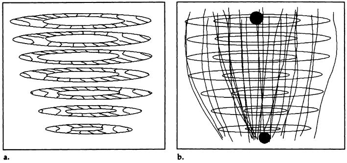
The three sets of tag planes corresponded to three orthogonal Cartesian coordinate axes. Portions of a representative human image set are shown in Figure 1. The images were processed by means of a semiautomated software package (18) to define positions along the tag lines and around the endocardial and epicardial heart contours. A typical tag and contour data set for a healthy human after image processing is shown in Figure 2. For a tag separation in the reference state of 6.0 mm, approximately 12 tags were produced in the myocardium in each set. At a point separation along each tag of 1 mm, this produced more than 4,600 raw data points, of which every other point was used in the fitting.
Figure 1.
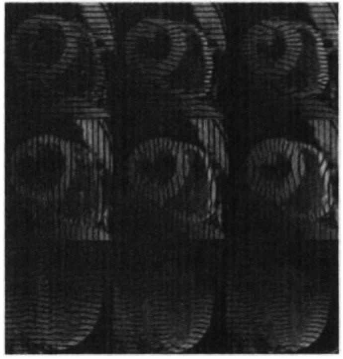
MR images (7.0/2.3, 15° flip angle) of an in vivo human heart of a healthy 30-year-old male volunteer obtained with the parallel-tagging and -imaging protocol. The progression (from left to right) through three phases in the cardiac cycle is shown: early, middle, and late systole. Two cardiac short-axis images and one long-axis image are shown; each displays tag lines from a different set of mutually orthogonal tag planes.
Figure 2.
(a) Typical 3D short-axis tag data set for x-displacement in an in vivo heart of a healthy volunteer. Image shows the appearance of the tags and the contours near end systole on seven short-axis image planes. (b) Typical 3D contour data set and the estimated prolate spheroidal centroid (upper gray circle) and apical focal point (lower black circle).
Field Fitting
In general terms, field fitting is a technique for estimation of the value of some parameter throughout a particular region of interest, given discrete samples of that parameter in and around that region. In displacement field fitting, the parameter of interest is the 3D displacement vector, and the samples are the values of one-dimensional displacement measured at points on tags in the deformed heart wall. Although field-fitting is generally applicable to any motion-detection method, it has been applied here to the analysis of three independent one-dimensional sets of displacement measurements from parallel-tagged MR images. This type of data is depicted in Figure 3, which illustrates a short-axis image and a deformed set of tags.
Figure 3.
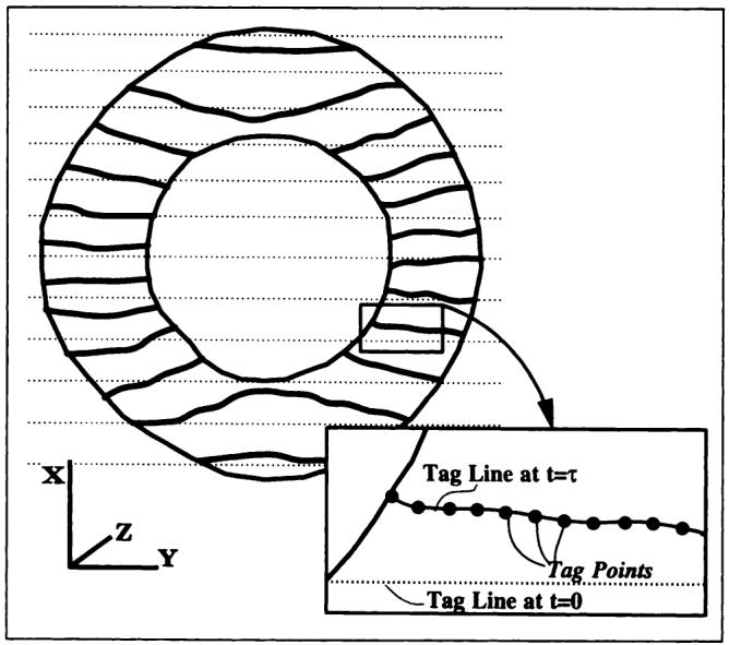
Depiction of a short-axis image at some time after initial tagging. Inset depicts an enlarged view of one deformed tag line after detection of tag points at 1-mm intervals.
The key concept of the method is shown in Figure 4. In three dimensions, each observed tag line represents the intersection of a deformed tag surface with the two-dimensional image plane. The tag surface results from the deformation of an initially flat tag plane. The figure depicts a tag surface within the heart wall that is cut by four parallel image planes. In each plane, tag points were marked along tag lines between the endocardial and epicardial heart contours. For each tag point on the deformed tag surface, the component of its displacement vector that was normal to the tag plane (Δx, in Fig 4) and its position were measured.
Figure 4.
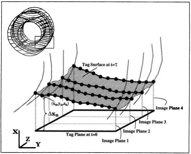
Deformation of a tag plane into a tag surface in 3D. The bold curves are the intersections of the tag surface within the heart wall with four vertical image planes. The enlarged dots on these curves are the tag points generated by means of an automated tag detection algorithm. Δxn represents the one-dimensional displacement associated with the nth tag point. The rectangle in the figure at the upper left shows the region of the heart depicted.
Reconstruction of the displacement field was performed by using the tag point displacement and position data to solve for the coefficients of a series expression that describes the field. This is analogous to use of digital sampling and Fourier analysis to reconstruct a continuous, one-dimensional signal. Here, this expression described the displacement throughout the entire left ventricle. In the simplest case, each unidirectional displacement data set was used to solve for an interpolation function for the displacement field in that one direction, independently of the motion in the other Cartesian directions. Once the three independent displacement field expressions were determined, they were used to compute the 3D displacement of any point in the deformed heart wall. At higher complexity, displacement data from multiple directions can be used simultaneously to solve for the full displacement vector field in an any coordinate system. The displacement field at each time frame was computed independently by using the time at which the tag planes were generated as the universal reference state.
Fitting to a power series in Cartesian coordinates
As an initial step, a first-order power series expansion in x, y, and z was used to remove the large-scale bulk motions and linear stretches and shears. This greatly increased the efficiency of the prolate spheroidal fitting by aligning the fixed centroid and long axis of the prolate spheroidal coordinate system at each time frame. In addition, large bulk deformations may cause the centroid or apical focus to intersect the myocardium, which would create a mathematical singularity within the heart wall; the Cartesian fit eliminates this problem. The expression for the displacement in x, Δx(x,y,z)(Fig 4), as a function of position (x,y,z) and unknown coefficients, ai, took the form Δx = a0 + a1x + a2y + a3z.
In vector notation, this can be written Δx = a · p, where a = [a0,a1,a2,a3] and p = [1,x,y,z]. (In this article, vectors are denoted with a lowercase bold italic font; tensors, uppercase bold italic; and scalars, plain italic.) For each sampled tag point (xn,yn,zn) each term in the vector p was evaluated and the x displacement value, Δxn, was measured. By considering the x displacements and p vectors for all tag points, a series of simultaneous equations was created and the unknown coefficients, a, were fitted by using singular value decomposition (a least-squares fitting method) (19). Independent series expressions for the y and z displacement fields were generated and fitted analogously.
Fitting to a power series in prolate spheroidal coordinates
To efficiently describe the curvilinear deformations expected in the heart, the first-order Cartesian fit was followed by a prolate spheroidal fit of the residual displacement fields. Figure 5 shows the prolate spheroidal coordinate system; λ is the radial component, ϕ is the longitudinal coordinate, θ is the circumferential angle, and f is the focal length. These are related to Cartesian coordinates by means of
| (1) |
| (2) |
and
| (3) |
For each prolate spheroidal coordinate displacement field, a series expansion with prolate spheroidal coordinates (λ,ϕ,θ) was created by using a generating function analogous to the spherical harmonic series:
| (4) |
where Pml is the associated Legendre polynomial function, N is the radial fitting order, L is the angular fitting order, and the unknown coefficients, ai, were numbered sequentially. For the typical tagging and imaging geometry and the typical image signal-to-noise characteristics, we determined that a fit with N = 1 and L = 4 was most appropriate for this data density (20) and generated 50 free-fitting parameters per coordinate direction.
Figure 5.
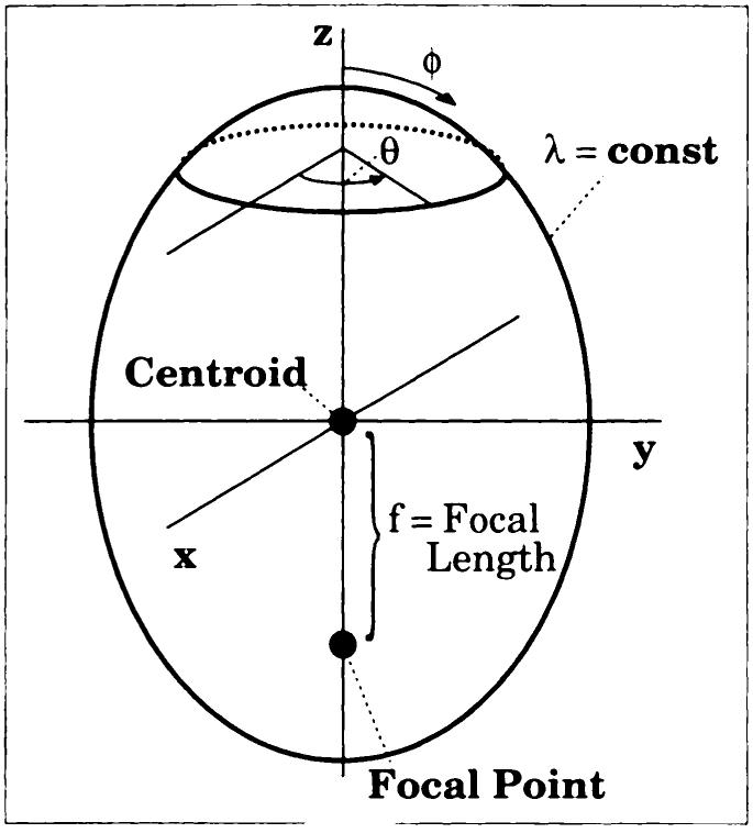
Prolate spheroidal coordinate system. Surfaces of constant λ are ellipsoids and surfaces of constant longitudinal coordinate ϕ are hyperboloids. const = constant.
To fit for the coefficients of the prolate spheroidal series expansions from measurements of displacement in the Cartesian coordinate directions, the measured displacements were projected onto the local prolate spheroidal axes. The infinitesimal displacements in Cartesian and prolate spheroidal coordinates are related by means of the following directional derivatives:
| (5) |
| (6) |
and
| (7) |
which can be expressed in vector notation as
| (8) |
where δx = [δx,δy,δz], δλ = [δλ,δϕ,δθ], and J is the Jacobian matrix for this coordinate transformation.
For a, b, and c, defined as the vectors of unknown coefficients for the δλ, δϕ, and δθ expressions, respectively, and p, the vector of 50 series terms derived from the generating function, Δλ = a · p, Δϕ = b · p, and Δθ = c · p (the a vector for the Cartesian fit and the a vector here are different). For the case in which the Cartesian axes (as defined by the three orthogonal sets of tag normal vectors) are centered and aligned with the prolate spheroidal coordinate system as described in Equations (1)-(3), the measured Cartesian displacements can be expressed as
| (9) |
| (10) |
| (11) |
and
| (12) |
where now α = [a0, … ,a49,b0, … ,b49,C0, … ,C49] and ρx = [J00P0, … J00P49, … J01P49,J02P0, … J02P49]. The vectors ρy and ρz were defined analogously. Similar to the method of solution of the Cartesian power series coefficients above, each measured displacement value was collected into a single row vector, Δx, and the corresponding ρ vectors were inserted as columns in a matrix P. The unknown coefficients, α, were then solved for by using the equation Δx = α · P.
In this way, all the unknown coefficients can be solved for simultaneously by using all available tag data and singular value decomposition. Although, for finite deformations, the relations between the displacements in x, y, and z and those in λ, ϕ , and θ are not exact, the simultaneous least-squares fitting will always result in the optimal fit of the given displacement data to the series expansion.
The fitting procedure was performed independently for each time frame in the data set. Because the heart geometry changes throughout the cardiac cycle, a new prolate spheroidal coordinate system was calculated for every time frame on the basis of the measured epicardial contour point data. This was done first by estimating the three coordinates of the centroid and the three coordinates of the apical focus (point on the long axis, toward the apex, at a distance of a focal length from the centroid) and by computing a least-squares optimal λ value at this centroid and apical focus for the given set of epicardial left ventricle contour points. Within an iteration loop, the six coordinates were then independently adjusted until a combination of centroid and focal point coordinates and the radial coordinate λ were derived that produced a prolate spheroid with the smallest fitting error to the measured left ventricle contour points.
Variation of the prolate spheroidal coordinate centroid and apical focus required that Equation (8) be modified to account for the coordinate transformation necessary to align the axes of the new spheroidal coordinate system with those defined by the normal vectors to the undeformed tag planes. For the transformation to the new coordinate system x′, defined with the rotation matrix R such that x′ = R · x, Equation (8) becomes δx = R-1Jδλ. This modification was used throughout the derivation. In addition, this formalism permitted 3D reconstruction from sets of images with arbitrary tag normal vectors, as long as three dimensions were spanned.
Computing strains at material points
A material point is defined as an infinitesimal volume of myocardial tissue. The mechanical state at a material point in the heart at any given imaging time is fully described by means of its deformation gradient tensor, F, according to dx = FdX, where x are the coordinates of the point in the deformed state and X are its coordinates in the reference state (21).
F was calculated from the displacement gradient tensor ▽u, which was computed numerically by taking partial derivatives of the displacement expressions with respect to the three coordinate directions. Because the terms in the series expansion were computed on the basis of the coordinates of the tag points in their deformed state, ▽u described the motion from the deformed state back to the undeformed state when the tags were created. Thus, to compute F from ▽u requires an inverse operation: F = (I − ▽u)−1, where I is the identity tensor. The Lagrangian finite strain tensor, E, can then be computed from E = ½(FTF − I), where the superscript T denotes matrix transposition.
For both the mathematical and experimental models, a set of material points was defined within the heart wall in the first imaging time frame and 3D displacements and deformations were evaluated over time at these points as they moved through space. A mesh of 96 material points regularly spaced in λ, ϕ, and θ was selected on the basis of the imaging section locations and the shape of the heart. The material-point locations at the first time frame were constrained longitudinally by the most basal and most apical short-axis image sections and radially by the endocardial and epicardial contours. The interpolation of the contour boundaries between image section locations was achieved by fitting the left ventricle epicardial and endocardial contour points of the first time frame to a fourth-order prolate spheroidal coordinate expansion for λ as a function of the two angular coordinates.
Analytical Test Case
To test the method with a known deformation field, a realistic, computer-generated deformation model was constructed. We adapted to prolate spheroidal coordinates an axisymmetrically deformative cylinder model described by Young and Axel (5), which was based on 3D strains measured by means of cine radiography of the anterolateral free wall of the left ventricle with implanted metallic beads (22). The governing equations that describe the deformed coordinates (λ,ϕ,θ) as a function of the initial coordinates (Λ,Φ,Θ) and the deformation parameters were as follows:
| (13) |
| (14) |
and
| (15) |
where A is the axial rotation at the equator, B is the torsion around the central axis, C is the transmural twist, D is the axial stretch, E is the transmural-longitudinal shear, f is the focal length of the prolate spheroidal coordinate system, Vol(λ) is the volume within a prolate spheroidal shell of constant λ, and “endo” denotes endocardial measurement. Deformation in the radial component, λ, was limited to a volume-conserving (incompressible) contraction mode by setting α = 1. The initial and deformed short-axis endocardial equatorial radii, fsinh(Λendo) and fsinh(λendo), were chosen to approximate realistic heart geometry and resulted in an ejection fraction of ∼50%. The prolate spheroidal deformation parameters are listed in Table 1.
Table 1.
Axisymmetric Deformation Model Parameters on a Prolate Spheroid
| Symbol | Value | Description |
|---|---|---|
| f sinh(Λendo) | 20.0 mm | Undeformed equatorial endocardial radius |
| f sinh(λendo) | 14.7 mm | Deformed equatorial endocardial radius, contraction |
| A | 9.17° | Axial rotation at the equator |
| B | 0.3°/mm | Torsion around the central axis |
| C | −0.28°/mm | Transmural twist |
| D | 0.8 | Axial stretch |
| E | 0.01 | Transmural-longitudinal shear |
Bulk motions and linear deformations that incorporate ellipticalization (the change in cross-sectional shape of the left ventricle from a circle at end diastole to an ellipse at end systole) and shears in x, y. and z were then superimposed on the axisymmetric modes in the manner of Arts et al (23). The magnitudes of these additional modes were chosen to provide the overall model with approximately physiologic rigid body motions and to reproduce those deformations observed by Arts et al (23). These deformation values are listed in Table 2. Image prescription error, which occurs when the central axis of the imaging volume is not coincident with the long axis of the left ventricle, was also simulated with representative values of 5° offset about the x axis and of 8° offset about the y axis.
Table 2.
Cartesian Deformation Parameters
| Symbol | Value | Description |
|---|---|---|
| Δ x | 1 mm | Translation in x |
| Δ y | 2 mm | Translation in y |
| Δ z | 4 mm | Translation in z |
| Rotx | 7° | Rotation about the x axis |
| Roty | 4° | Rotation about the y axis |
| k xy | 0.05 | Shear in the xy plane |
| k xz | 0.05 | Shear in the xz plane |
| k yz | 0.07 | Shear in the yz plane |
| k ell | 0.05 | Ellipticalization in the xy plane |
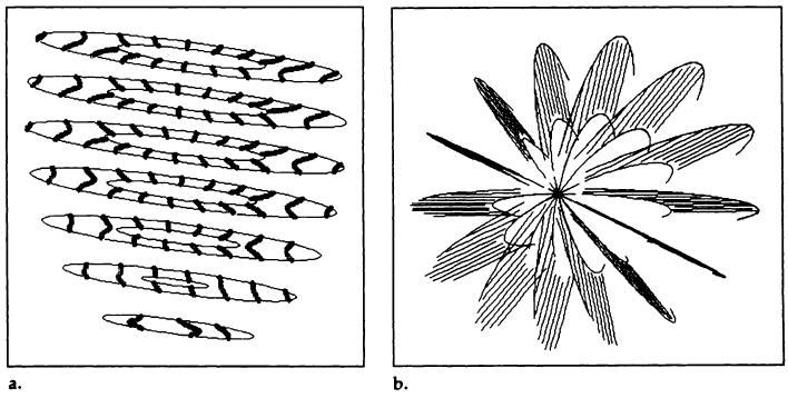
Seven image sections and 10 tag planes were simulated for each image set. Separation between adjacent tag points along a given tag was fixed at 2 mm. Throughout the entire 3D data set, this produced ∼2,400 tag points. The prolate spheroidal deformation model is shown in Figure 6.
Figure 6.
Simulated (a) short-axis and (b) long-axis tag data sets for the prolate spheroid model. Physiologic deformation modes with added Cartesian motions were modeled for seven image sections and 10 tag planes in each view. The angles of tilt are due to simulated image prescription error.
Human Data Sets
Ten healthy human volunteers gave informed consent and underwent imaging with a 1.5-T scanner (Signa; GE Medical Systems, Milwaukee, Wis). A cine breath-hold imaging sequence with parallel tags was used (8). Eighteen acquisitions were performed in each subject during a breath hold. Volunteers underwent imaging at end expiration in the supine position with a flexible surface coil wrapped around the left side of the chest.
The imaging parameters for each section were a repetition time of 7.0 msec and an echo time of 2.3 msec (7.0/2.3, fractional echo), a 15° flip angle, 110 phase encoding steps, 1.25 × 2.9 × 7 mm voxels, one signal acquired, and five phase-encoded views per movie frame (35 msec time resolution). The tagging pulse consisted of five nonselective radio-frequency pulses with relative amplitudes of 0.7, 0.9, 1.0, 0.9, and 0.7 separated by spatial modulation of magnetization (2) encoding gradients to achieve a tag spacing of 6 mm. The tagging tip angle was tuned to achieve a 180° flip angle.
Monte Carlo Simulations
A representative human data set was fitted; the reconstructed displacement field and heart geometry were then used to generate a physiologic noise-free parallel tag data set. The effect of uncertainty in tag point position on the final material-point tracking predictions was evaluated by using a Monte Carlo simulation (19). One-dimensional Gaussian noise profiles with 0.25–1.00-mm standard deviation were added to the Δx, Δy, and Δz data sets, and the resultant 3D material-point trajectories were computed for the 96 material points for 100 trials. A single root-mean-square deviation (RMSD) value was computed for each point from the 3D distribution of the cloud of estimated point trajectories around the expected location.
RESULTS
Two measures of the displacement field-fitting performance were evaluated with the prolate spheroidal deformation model: tracking and fitting. The 3D tracking performance was evaluated by comparing the estimated material-point trajectories derived from the field-fitting reconstruction to the exact solution computed from the deformation model of Equations (13)-(15). The mean absolute value and the standard deviation of the tracking error were computed for the set of 96 material points. The fitting performance was evaluated by computing the standard deviation of the error (SDE; around a mean error of 0) between the estimated and the measured one-dimensional displacements at each tag point. Thus, the fitting performance reflects the ability of the reconstruction to account for the variations in the displacement field at the locations where the measurements were made, whereas the tracking performance reflects both the quality of the fitting and the interpolation of the displacement field between the measurement locations.
Mathematical Deformation Model Results
The SDE of the fit to the ∼2,400 model tag data points was 0.095 mm. This is on the order of the expected uncertainty in the determination of tag point displacements for typical in vivo data sets (16,17). This implies that the fitting error for a human data set will be dominated by the uncertainty in the tag point displacement data rather than by error in reconstruction of the displacement field at the measurement locations.
The 3D tracking error for the set of 96 material points was 0.28 mm ± 0.i6 (mean ± standard deviation). The relatively large value of the 3D tracking error (∼0.3 mm) compared to the SDE of the fit (∼0.1 mm) suggests that further improvements to the reconstruction can be made by increasing the tag density and number of fitting parameters. The corresponding circumferential strain errors at the 96 material points were 0.006 ± 0.012 for a mange of −0.25 to 0.06, the longitudinal strain errors were 0.0003 ± 0.0070 for a range of −0.23 to −0.08, and the midwall radial strain errors were 0.017 ± 0.026 for a range of midwall radial strains of 0.18–0.52. The high accuracy of the strain estimations, even where 3D tracking errors were ∼0.3 mm, is due to the correlation of tracking errors between neighboring myocardial regions. These errors and standard deviations are well below the threshold necessary to detect motion abnormalities in the ischemic heart wall (24).
In Vivo Human Heart Results
The SDE of the fit (a mean error of ∼0) to the tag data at 228 msec after the electrocardiograph R wave in the 10 subjects was 0.36 mm ± 0.06 (mean SDE ± standard deviation SDE). This reflects both the error in reconstruction of the displacement field, as seen in the fit results for the mathematical model, and the uncertainty in the determination of the tag point locations. The accuracy of the fitting can be illustrated by the ability to reconstruct the positions of deformed tags. The fitted 3D displacement field was used to generate points that started from the reference state tag plane locations and moved into the image plane at 228 msec into systole. Figure 7 shows representative short- and long-axis human cardiac images obtained at 228 msec into systole and demonstrates the agreement between the predicted locations of the tag points and the actual tags on the MR images.
Figure 7.
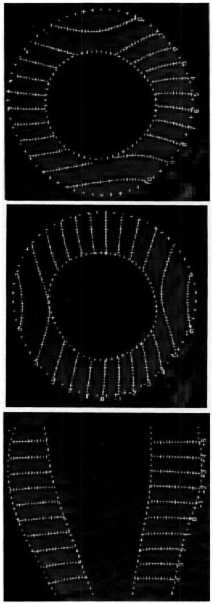
Short- and long-axis MR images (7.0/2.3, 15° flip angle) of a human heart obtained in a healthy, 21-year-old male volunteer at 228 msec into systole overlaid with tag point locations predicted from the 3D field fit.
Monte Carlo Noise Analysis
The precision of the fitting algorithm was tested by using a Monte Carlo simulation as described in Monte Carlo Simulations in Materials and Methods. The RMSD of the computed material-point position increased linearly as a function of input noise level as shown in Figure 8. It was determined that the scatter of points around the expected value was isotropic. The RMSDs at the endocardial and epicardial material points were equal and were greater than the RMSD at the midwall. At an input noise standard deviation of 0.5 mm, the midwall RMSD tracking error was 0.077 mm ± 0.015, and the endocardial and epicardial RMSD was 0.126 mm ± 0.030. The RMSD computation with a subset that consisted of 50 trials produced results that were not significantly different, which suggests that 100 trials were sufficient to obtain a stable convergence of the estimate in tracking precision.
Figure 8.
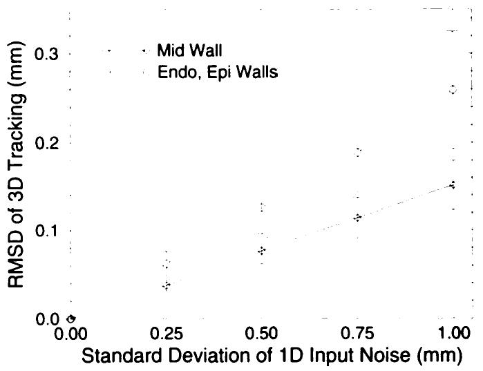
RMSD of the computed material-point position as a function of input noise level on a human heart geometry and deformation field. The distribution of tracked points formed an isotropic cloud around the noise-free reference trajectory. The RMSD of the distribution about the endocardial and epicardial material points were the same and were larger than those about midwall material points. The error bars correspond to the standard deviation in the RMSD for the 100 Monte Carlo trials. 1D = one-dimensional.
DISCUSSION
The combination of parallel-tag MR imaging and displacement field fitting is am accurate and robust method for reconstruction of the 3D deformation field throughout the entire left ventricle. Because of its reliance on parallel-tag data, the displacement field-fitting method is inherently less susceptible to tag- and contour-detection errors than were previous MR imaging reconstruction schemes, because only the center line of any tag need be determined during image analysis. The incorporation of a greater number of points along each tag line increases the sampling density throughout the heart compared with the sampling density obtained with techniques that use only those points located at intersections between tags or between tags and myocardial contours.
The fitting of displacement fields can also be realized by using other methods, which include energy minimization techniques (5,25). In this approach, the fits can be computed numerically for a predefined set of material points (nodes), and interpolation between these points is accomplished by means of linear on finite element interpolation functions. Although field fitting by solving for series coefficients has some mathematical similarities to energy minimization and other methods, the series method has several advantages. First, it is independent of material strain energy models. Second, the global fit provides the ability to express the 3D deformation at any myocardial point with a relatively small number of parameters, independently of a predefined set of material points.
The field-fitting approach is immediately suitable for other methods of 3D strain analysis in which motions in multiple directions are independently measured. For example, three sets of velocity-encoded images (26) could be used to solve for a set of expressions that describe the velocity field throughout a prescribed region of interest in a manner analogous to that described for tag-based displacement fields. This would have the advantage of smooth interpolation of the velocity field. Grid tag data sets cam also be analyzed by interpreting the grid as two independent sets of parallel tags.
We have demonstrated the application of displacement field fitting by using an analytical series expression for the analysis of tagged MR imaging cardiac data. The important features of this method are that it allows all the available tag data to be considered and not just points at tag-tag on tag-contour intersections, it allows the determination of the local 3D deformation gradient tensor at any point in the heart wall, it has predictable noise propagation characteristics, and it is suitable for the analysis of both grid-and parallel-tagged MR data. This last property is important in light of recent advances in cardiac breath-hold imaging that are virtually free of motion artifact and in which only parallel tags are produced.
The cascade of a first-order Cartesian basis set fit and a geometrically more appropriate prolate spheroidal fit enable reconstruction of material-point trajectories to within 0.3 mm for a physiologic deformation model. At late systole in 10 healthy human subjects, tag displacement data was reconstructed with an average error of 0.00 mm ± 0.36, in which the standard deviation of the error approximately matched the expected uncertainty in the determination of the in vivo tag point displacements. This suggests that all the displacement information contained in the tag data has been accounted for in the reconstruction. The combination of rapidly acquired parallel-tagged MR images and field-fitting analysis is a valuable tool for cardiac mechanics research and for the clinical assessment of cardiac mechanical function.
Acknowledgments
The authors gratefully acknowledge Andrew Douglas, PhD, for thoughtful discussions and Carlos Lugo-Olivieri, MD, for assistance in acquisition of the human heart data.
1 Supported in part by grants HL45090 and HL45683 from the National Institutes of Health, by a fellowship from the Merck Sharp and Dohme Corp (C.C.M.), and by a Whitaker Foundation Biomedical Engineering Research Grant.
Abbreviations
- 3D
three-dimensional
- RMSD
root-mean-square deviation
- SDE
standard deviation of the error.
References
- 1.Zerhouni EA, Parish DM, Rogers WJ, Yang A, Shapiro EP. Human heart: tagging with MR imaging—a method for noninvasive assessment of myocardial motion. Radiology. 1988;169:59–63. doi: 10.1148/radiology.169.1.3420283. [DOI] [PubMed] [Google Scholar]
- 2.Axel L, Dougherty L. MR imaging of motion with spatial modulation of magnetization. Radiology. 1989;171:841–845. doi: 10.1148/radiology.171.3.2717762. [DOI] [PubMed] [Google Scholar]
- 3.Mosher TJ, Smith MB. A DANTE tagging sequence for the evaluation of translational sample motion. Magn Reson Med. 1990;15:334–339. doi: 10.1002/mrm.1910150215. [DOI] [PubMed] [Google Scholar]
- 4.Bolster BD, MeVeigh ER, Zerhouni EA. Myoeardial tagging in polar coordinates with striped tags. Radiology. 1990;177:769–772. doi: 10.1148/radiology.177.3.2243987. [DOI] [PMC free article] [PubMed] [Google Scholar]
- 5.Yount AA, Axel L. Three-dimensional motion and deformation of the heart wall: estimation with spatial modulation of magnetization—a model-based approach. Radiology. 1992;185:241–247. doi: 10.1148/radiology.185.1.1523316. [DOI] [PubMed] [Google Scholar]
- 6.O'Dell WG, Schoeniger JS, Blackband SJ, McVeigh ER. A modified quadrapole gradient set for use in high resolution MRI tagging. Magn Reson Med. 1994;32:246–250. doi: 10.1002/mrm.1910320215. [DOI] [PMC free article] [PubMed] [Google Scholar]
- 7.Fischer SE, MeKinnon GC, Maier SE, Boesiger P. Improved myocardial tagging contrast. Magn Reson Med. 1993;30:191–200. doi: 10.1002/mrm.1910300207. [DOI] [PubMed] [Google Scholar]
- 8.McVeigh ER, Atalar E. Cardiac tagging with breath hold cine MRI. Magn Reson Med. 1992;28:318–327. doi: 10.1002/mrm.1910280214. [DOI] [PMC free article] [PubMed] [Google Scholar]
- 9.Atkinson DJ, Edelman RR. Cineangiography of the heart in a single breath hold with a segmented turboFLASH sequence. Radiology. 1991;178:357–360. doi: 10.1148/radiology.178.2.1987592. [DOI] [PubMed] [Google Scholar]
- 10.Moore CC, Reeder SB, McVeigh ER. Tagged MR imaging in a deforming phantom: photographic validation. Radiology. 1994;190:765–769. doi: 10.1148/radiology.190.3.8115625. [DOI] [PMC free article] [PubMed] [Google Scholar]
- 11.Young AA, Axel L, Dougherty L, Parenteau CS. Validation of tagging with MR imaging to estimate material deformation. Radiology. 1993;188:101–108. doi: 10.1148/radiology.188.1.8511281. [DOI] [PubMed] [Google Scholar]
- 12.McVeigh ER, Zerhouni EA. Noninvasive measurement of transmural gradients in myocardial strain with magnetic resonance imaging. Radiology. 1991;180:677–683. doi: 10.1148/radiology.180.3.1871278. [DOI] [PMC free article] [PubMed] [Google Scholar]
- 13.Rogers WJ, Shapiro EP, Weiss JL, et al. Quantification of and correction for left ventricular systolic long-axis shortening by magnetic resonance tissue tagging and slice isolation. Circulation. 1991;84:721–731. doi: 10.1161/01.cir.84.2.721. [DOI] [PubMed] [Google Scholar]
- 14.Moore CC, O'Dell WG, McVeigh ER, Zerhouni EA. Calculation of three-dimensional left ventricular strains from bi-planar tagged MR images. JMRI. 1992;2:165–175. doi: 10.1002/jmri.1880020209. [DOI] [PMC free article] [PubMed] [Google Scholar]
- 15.Moore CC, McVeigh ER, Mebazaa A, Zerhouni EA. Use of striped radial tagging to measure three-dimensional endocardial and epicardial deformation throughout the canine left ventricle during isehemia (abstr) JMRI. 1993;3(P):124. [Google Scholar]
- 16.Atalar E, McVeigh ER. Optimum tag thickness for the measurement of motion by MRI. IEEE Trans Med Imaging. 1994;13:152–160. doi: 10.1109/42.276154. [DOI] [PMC free article] [PubMed] [Google Scholar]
- 17.Bazille A, Guttman MA, McVeigh ER, Zerhouni EA. Impact of semiautomated versus manual image segmentation errors on myocardial strain calculation by MR tagging. Invest Radiol. 1994;29:427–433. doi: 10.1097/00004424-199404000-00008. [DOI] [PMC free article] [PubMed] [Google Scholar]
- 18.Guttman MA, Prince JL, McVeigh ER. Tag and contour detection in tagged MR images of the left ventricle. IEEE Trans Med Imaging. 1994;13:74–88. doi: 10.1109/42.276146. [DOI] [PubMed] [Google Scholar]
- 19.Press W, Flannery B, Teukolsky S, Vetterling W. Numerical recipes in C: the art of scientific computing. Cambridge University Press; Cambridge, England: 1988. [Google Scholar]
- 20.O'Dell WG, Moore CC, McVeigh ER. Proceedings of the Society of Magnetic Resonance. Society of Magnetic Resonance; Berkeley, Calif: 1994. Optimization of displacement field fitting for 3D deformation analysis; p. 1483. [Google Scholar]
- 21.Malvern LE. Introduction to the mechanics of a continuous medium. Prentice Hall; Englewood Cliffs, NJ: 1969. [Google Scholar]
- 22.McCulloch AD, Omens JH. Nonhomogeneous analysis of three-dimensional transmural finite deformation in canine left ventricle. J Biomech. 1991;24:539–548. doi: 10.1016/0021-9290(91)90287-w. [DOI] [PubMed] [Google Scholar]
- 23.Arts T, Hunter W, Douglas A, Muijtjens A, Reneman R, Corday E. Description of the deformation of the left ventricle by a kinematic model. J Biomech. 1992;25:1119–1127. doi: 10.1016/0021-9290(92)90068-c. [DOI] [PubMed] [Google Scholar]
- 24.Lugo-Olivieri CH, Moore CC, Poon EGC, Lima JAC, MCVeigh ER, Zerhouni EA. Proceedings of the Society of Magnetic Resonance. Society of Magnetic Resonance; Berkeley, Calif: 1994. Temporal evolution of three dimensional deformation in the isehemic human left ventricle: assessment by MR tagging; p. 1482. [Google Scholar]
- 25.Denney TS, Jr., Prince JL. Proceedings of the IEEE Workshop on Non-rigid and Articulate Motion, Austin, Texas 1994. IEEE Computer Society; Los Alamitos, Calif: 1994. 3D displacement field reconstruction on an irregular domain from planar tagged cardiac MR images. [Google Scholar]
- 26.Pelc NJ. Book of abstracts: Society of Magnetic Resonance in Medicine 1991. Society of Magnetic Resonance in Medicine; Berkeley, Calif: 1991. Myocardial motion analysis with phase contrast one MRI; p. 17. [Google Scholar]


