Impact of Semiautomated versus Manual Image Segmentation Errors on Myocardial Strain Calculation by Magnetic Resonance Tagging

Abstract

Rationale and Objectives

Accurate image segmentation is essential for the study of mechanical properties of the myocardium by tagged magnetic resonance imaging (MRI). The relative accuracy of three methods of segmentation of myocardial borders and tags and their impact on myocardial strain calculations were evaluated.

Methods

Radially tagged, spin-echo magnetic resonance (MR) images of dog hearts were segmented manually, automatically, and semiautomatically. The variability of segmentation methods was separately determined for myocardial contours and tags. Error propagation assessment for strain calculation was estimated.

Results

The variability of the segmentation of the contours was five times greater than that of the tags. The error propagation is nonuniform in all directions, maximal for the radial component of strain.

Conclusion

Errors in the segmentation of myocardial contours are significantly greater than those of the tags. Strain calculations should be based solely on segmentation of MR tags to avoid significant errors, particularly in radial strain estimates.

Myocardial tagging techniques are potentially powerful tools in the study of the myocardial properties in health and disease.^1-6 In the past, finite element analysis of the deformation or strain parameters of the myocardium has been possible, on a limited basis, only with surgically implanted radiopaque markers or sonomicrometers.^7-11 With magnetic resonance (MR) tagging, cardiac strain can be measured noninvasively.^13,14

However, the accuracy of such measurements depends heavily on our ability to accurately segment and track specific volume elements of myocardial tissue on MR images throughout contraction. Identification of tags and myocardial borders is a critical step in this process. In this report, we assess the performance of a fully automated segmentation program developed in-house against that of manual and semiautomated approaches and their potential impact on strain calculation.¹⁴

Materials and Methods

Image Acquisition

Five healthy dogs were examined with a 1.5-Tesla MR machine (Signa, General Electric, Milwaukee, WI). They were anesthetized with pentobarbital (35 mg/kg) after being sedated with acepromazine and were ventilated with a Harvard respirator. The animals were placed in a head coil (30 cm diameter), and an electrocardiogram was obtained using external electrodes on the chest. The protocol, in agreement with National Institute of Health guidelines, was approved by the Johns Hopkins Animal Care and Use Committee.

The images were acquired using cardiac gating. The R wave triggered a tagging pulse sequence, followed by a multiscan, multiphase spin-echo sequence (echo time [TE]: 14 msec; repetition time [TR]: 2 RR intervals). Two orthogonal sets of images were obtained: four short-axis images with six equiangular radial tags, and six radially distributed long-axis images with six parallel tags, of which the four middle ones spatially corresponded to the short axis images of the first series, as shown in Figure 1. Images were obtained at four equidistant time points during systole. The scan thickness was 10 mm, with a 3-mm gap, the field of view was 24 to 28 cm, the matrix was 256 × 128, and the pixel size was 1 × 2 mm. With 2 Nex, the total imaging time was about 50 minutes.

Fig. 1.

The tagging planes for the (A) short-axis series correspond to the imaging planes of the (B) long-axis series. The four middle tagging planes of the (B) long-axis series correspond to the imaging planes for the (A) orthogonal short-axis series.

Image Analysis

Only the 16 images of each short-axis series were considered for this study. The images were transferred on magnetic tape to a SUN 4/280 workstation (SUN Microsystems, Mountain View, CA) equipped with a TAAC-1 graphic accelerator board. The images were compressed to 8 bits and interpolated onto a 1-mm pixel grid.

Manual segmentation was performed separately by two observers (A.B.: Observer 1; M.A.G: Observer 2). Each observer was free to choose the display window setting. Cinematic display also was available to the observers because it facilitates the identification of endocardial and epicardial borders. Each observer first evaluated image quality and was asked to exclude all images considered suboptimal for manual segmentation. Reasons for exclusion were noted on a protocol sheet.

The manual segmentation was done with a mouse, with the contour displayed as a series of dots. The endocardial contour was defined first, then the epicardial contour, and finally, the center line of the 12 radial tags intersecting the left ventricular myocardium. To assess the intraobserver variability, Observer 1 repeated the manual segmentation 1 month later.

The details of the in-house automated segmentation algorithm used in this study have been described previously,¹² but we will briefly review them. The region of the left ventricle is isolated in the image by the operator who sets a circular region of interest with the center matching approximately that of the left ventricular cavity. The first step of the program is a smoothing operation using a median filter. Because the tags cause breaks in the myocardial contours, a morphologic closing operation is applied using a linear structuring element orthogonal to the expected tag stripe direction. This procedure removes the tags without appreciably affecting the contour shape. A Sobel edge enhancement filter is applied in the x and y direction on the closed image, thereby defining the orientation and the magnitude of the gradient. The image is evaluated along 64 rays, emanating from the center of the region of interest. Each search ray is separated by an angle of about 6°.

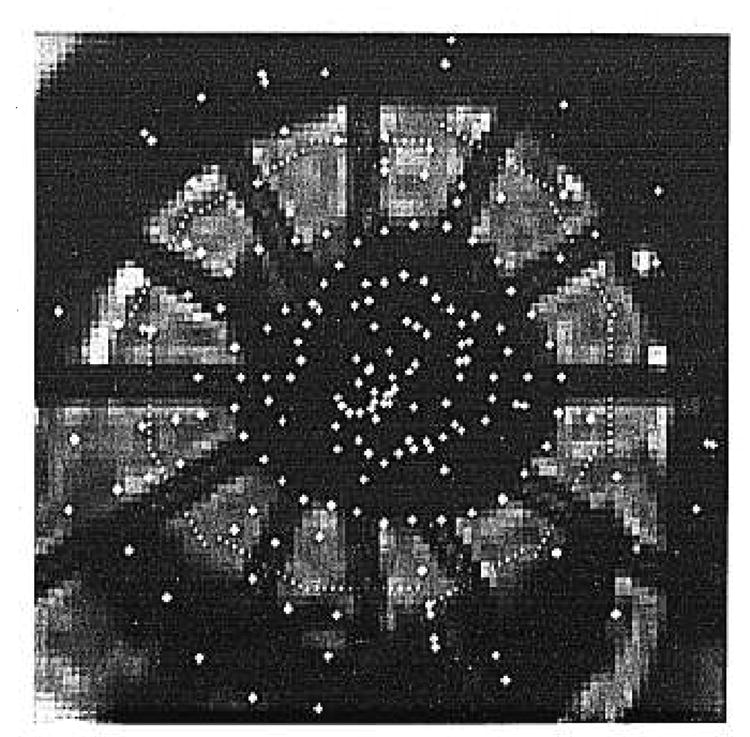
To define the possible myocardial border candidate points, the program considers local maximums on 3 pixels, reading along the search rays on the gradient magnitude image. Separate pools of candidate points are formed for the endocardial and epicardial borders, as shown in Figure 2. For the endocardial borders, the program considers only the positive local maxima of the gradient as candidate points, corresponding to the transition between the signal void of the left ventricular cavity and the intermediate signal of the myocardium. For the epicardial borders, the program considers both the positive local maxima and the negative local maxima of the gradient to account for two types of findings: 1) the transition between lung (low signal) and myocardium (intermediate signal) or 2) the transition between fat (high signal) and myocardium. The best candidate points are chosen by dynamic programming with various cost functions. These functions have been designed to emphasize the spatial coherence between two adjacent points on the same slice, considering the magnitude and the direction of the gradient and the smoothness of the contour. Two other cost functions are unique to this program because they account for the spatial coherence of neighboring points in two spatially adjacent slices and the temporal coherence between two temporally adjacent slices. The dynamic programming algorithm chooses a candidate point on each ray, which minimizes the total cost of the contour. In this manner, we obtain endocardial and epicardial borders. A smoothing operation, using a median filter at threshold, is applied to the optimized contour to remove outliers from the myocardial contours.

Fig. 2.

Candidate pool for endocardial contour. Among them, the best points will be selected by dynamic programming using cost functions.

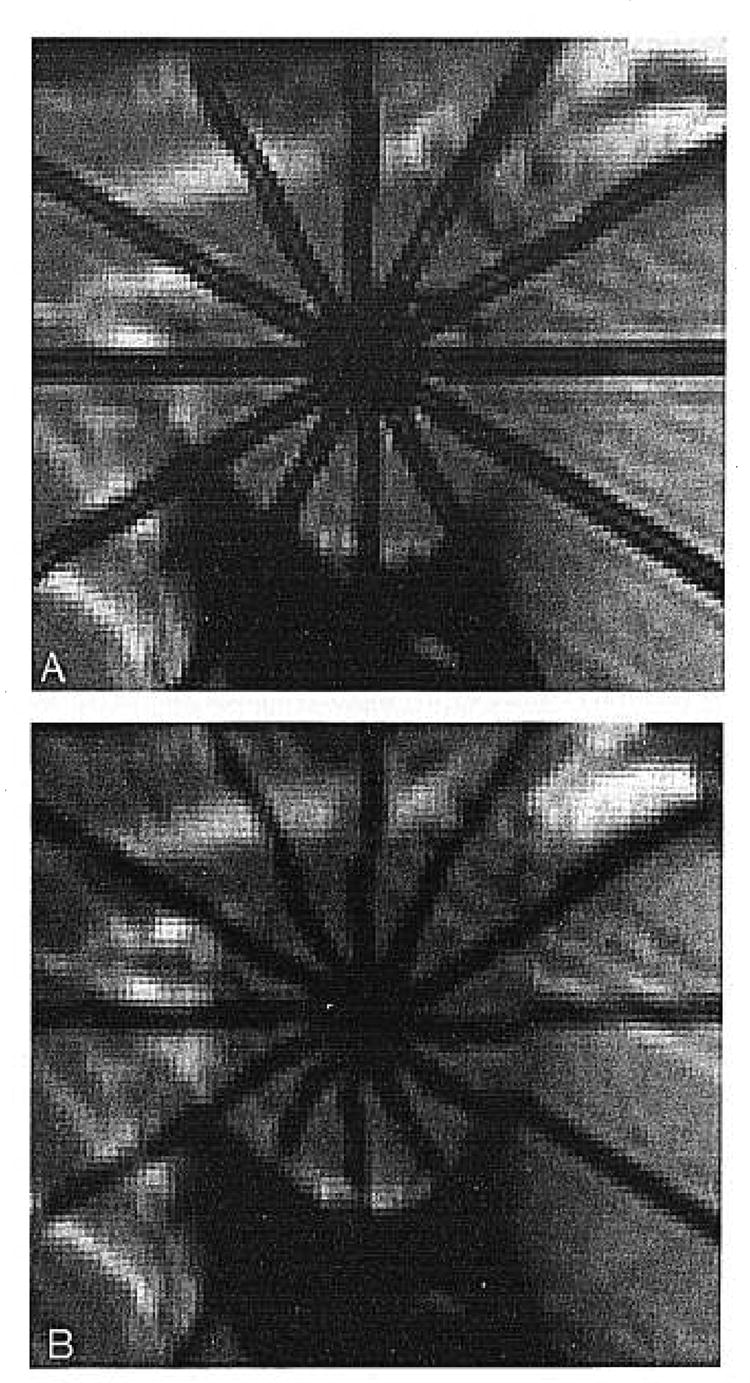
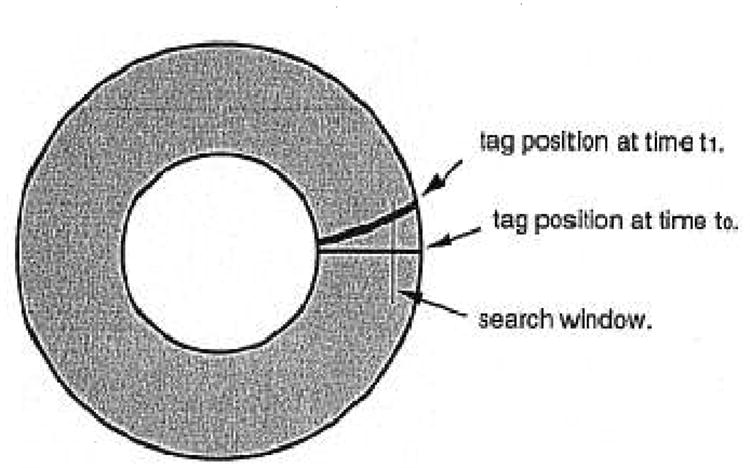
After the myocardial contours are defined, the tags are detected using the original unprocessed images. A pattern containing 12 radial lines is applied to match the expected position of the tags. An orthogonal 1-cm window is placed on each line on the outer third of the myocardium to determine the center line of the tag profile, as shown in Figure 3. This window enables tracking of the center line of the tag toward the epicardial and endocardial borders. A median filter is applied to obtain smooth tag lines, thereby displaying the fully automated segmented image (Fig. 4).

Fig. 3.

The search window is placed orthogonal to the initial tag position at time t⁰ to find the centerline of the same tag observed at time t¹.

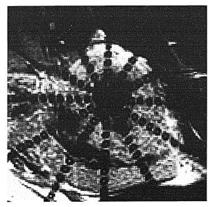
Fig. 4.

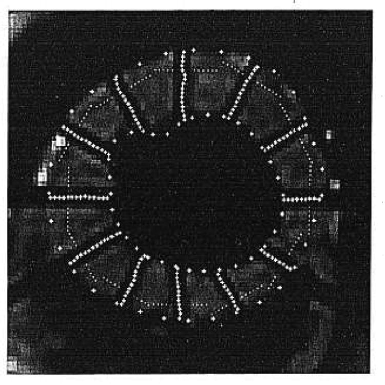
Final image after automated segmentation of the contours and of the tags.

For the semiautomated segmentation, the operator visually checks the accuracy of the points that have been automatically generated. The points that have been improperly positioned after automated segmentation can be modified manually throughout an interactive correction routine. After manual correction, all points are recomputed to fit the cost functions of the dynamic programming routine and rechecked visually.

The total time required for segmentation per image was recorded for each method.

Statistical Analysis

For the contours, we considered 64 sectors defined by an angle β, where β = 2π/64 (Fig. 5A). For each sector we considered the contour points placed by two observers (human, automated, or semiautomated). We measured the difference between the radius of each of the two points. If the point was missing in this sector for one of the observers, we performed a linear interpolation between the nearest neighbors.

Fig. 5.

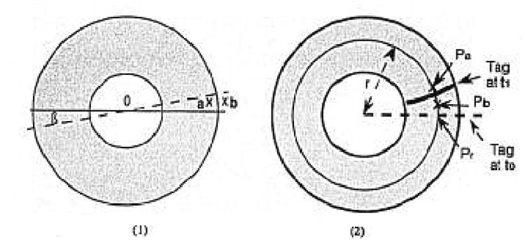
(A) a and b are the points positioned by two different observers for the eplcardial border in the β sector. The difference between the two radii O^a and O^b was measured. (B) P^r is placed on the “r” radius and on the virtual line defined by the initial position of the tag at time t⁰. P^a and P^b are the points placed on the “r” radius by two different observers to define the tag at time t¹. The P^r-P^a and P^r-P^b distances were measured.

For each tag, we superimposed a reference line corresponding to the initial position of the tag (at time t⁰). We define a “P^r” location on this reference line corresponding to the tag position at an “r” radius from the center, as shown in Figure 5B. We considered the points (P^a, P^b) placed by two observers (A,B) to define the tag position on the same “r” radius, at the time t¹. We compared the distance P^a-P^r and the distance P^b-P^r to evaluate the variability of the position around the tag. We repeated the measurement at 1-mm increments on the reference line between myocardial borders.

The differences were measured in millimeters, and the variability was calculated for each pair of observers. The intraobserver variability was tested on the “Observer 1a and Observer 1b” pair, and the interobserver variability was tested on pairs chosen among the three manually segmented series (Observer 1a, Observer 1b, Observer 2), the automated segmented series (auto), and the semiautomatically segmented series (semiauto).

Results

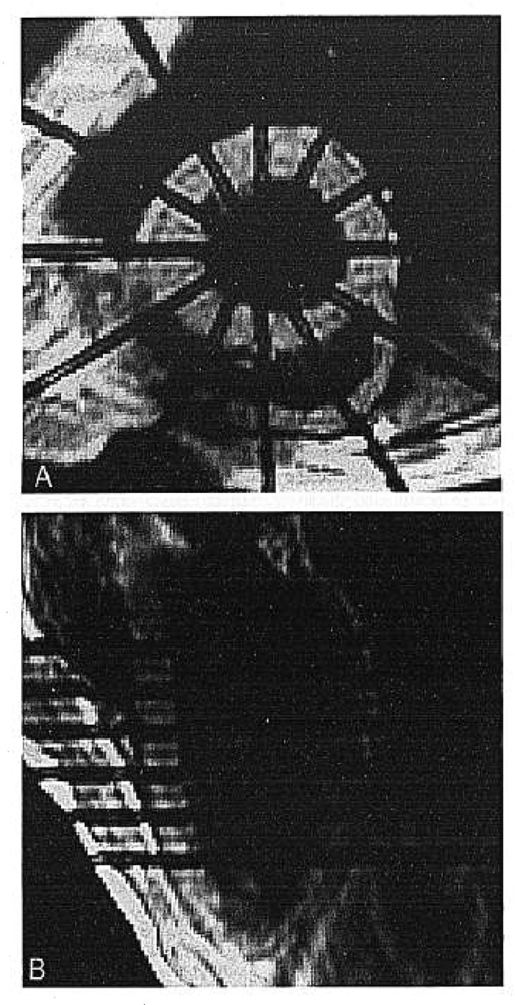
Among the 80 submitted images, 40 were considered optimal for analysis by both manual observers. There were several reasons for rejecting an image, including 1) poor quality of the image because of motion artifacts that blurred the contours; 2) premature fading of the tags on the last time frame; and 3) inappropriate position of the slice (too high or too low). Inappropriate position at the apex of the left ventricle was of concern in this study. Because of the radial pattern of the tags and their thickness, the intersection of the tags at the center could form a circle larger than the cavity at the most apical level, thus masking the endocardial border, as shown in Figure 6.

Fig. 6.

Apical slice observed at (A) t = 0 and (B) t = 200 msec. The intersection of the radial tags, especially on the first time frame, can obscure the endocardial border.

Manual Segmentation

Manual segmentation required an average of 10 minutes per image. Even for good quality images, difficulties were often experienced in deciding the proper position of the myocardial borders. Problems included 1) the heterogeneity of the myocardial signal (near turbulent blood signal in the ventricular cavity); 2) the lack of clear differentiation between epicardium and epicardial fat; 3) the absence of obvious delineation between the epicardial border and adjacent anatomic structures, such as the liver or chest wall; and 4) confusion created by the papillary muscle and its partial volume effect on adjacent slices.

However, the segmentation of the tags was easily accomplished, except when tags were fading toward end-systole.

Automated and Semiautomated Segmentation

One minute per image was needed to perform the automated segmentation, including the time required for the operator to set the circular region of interest around the left ventricle.

After visually checking the accuracy of the program, we found that 273 of 5120 (5.3%) points had to be corrected manually for the myocardial borders. Among these points, no statistically significant difference was found between the number of points belonging to the endocardial contours (57%) and those belonging to the epicardial contours (43%).

The determination of the center lines of the tags appeared to be excellent, and no manual correction was required.

The manual interactive correction of automated segmentation required 1 to 2 minutes per image.

Statistical Analysis

Contours

The statistical analysis was performed for 5120 (64 points × 40 images × 2 contours) measurements made 9 times (9 observer pairs). The values of the variability (variance) ranged between .09 and .29 mm. The corresponding standard errors values (SE) ranged from .1 to .54 mm.

The intraobserver variability appeared to be the lowest, whereas variability between different human observers was slightly higher (manual/manual pairs), indicating observer-dependent bias. The variability between human observers and the fully automated program was the highest (manual/automated pairs). The variability between the strictly manual series and the semiautomated (manual/semiautomated) series seemed to be slightly lower than the one found with the uncorrected automated program, but the difference was not significant (Table 1).

TABLE 1.

Statistical Analysis

Variability	Segmentation technique	Observer pair	SE (mm) Contour (n = 5,120)	SE (mm) Tag (n ≈ 4,800)
Intra-observer	manual/manual	1A/1B	0.31	0.09
Inter-observer	manual/manual	1A/2	0.42	0.11
		1B/2	0.46	0.12
	manual/automated	1A/auto	0.54	0.10
		1B/auto	0.51	0.10
		2/auto	0.52	0.13
	manual/semi-automated	1A/semi-auto	0.49	0.07
		1B/semi-auto	0.52	0.06
		2/semi-auto	0.47	0.08

SE: standard error.

SE values of tags are significantly lower than that of the contours (student unpaired t test: P < .0005).

Tags

The measurements were done for 480 (40 images × 12 tags) tags for 9 observer pairs. The number of points averaged about 10 points per tag, for a total of 4800 tag points. The variability values ranged between .009 and .016 mm; they were in the same range for all tested observer pairs and significantly lower than those of the contours (Student’s unpaired t test: P < .0005). The corresponding SE values ranged from .09 to .13 mm. The SE difference between the two groups (contours, tags) is significant (Student’s unpaired t test: P < .0005); on average the SE for the contours is five times greater than that for the tags.

If we display, in two dimension, the cloud of points representing the uncertainty around a tag point, we observe that this cloud is elliptical, with a radially oriented long axis, as shown in Figure 7. Thus, the radial component of strain is prone to greater error than is the circumferential component.

Fig. 7.

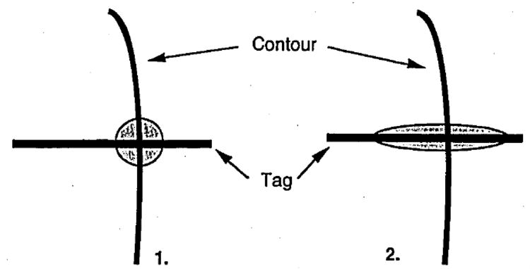
1) Initial hypothesis where the two-dimensional error repartition is random around the tag point. 2) Two-dimensional error repartition around the point in our study.

Discussion

In this study, we evaluated three different image segmentation methods (manual, automated, and semiautomated) without deciding which one was a priori the “gold standard.” No valid phantom to evaluate the absolute accuracy of segmentation methods in the beating heart has been designed. Thus, we chose to evaluate the variability of each method among several observer pairs.

The SE between different human observers is lower than that between the human observers and the fully automated program. This may be attributed to a basic difference in the appreciation of the contour location by human operators and the segmentation program. The window level settings play a significant role in this difference because they alter the human appreciation of the location of the border. For instance, the automated program consistently placed contour points inside those placed by the human observers. Presumably, the program analyzed edge gradients better than human observers because the program is based on the pixel values, rather than a subjective impression. Conversely, human observers can correct for localized lack of image information, such as the absence of a defined gradient (ie, at the left ventricle-right ventricle junction). Human observers can perform a discriminative interpolation because of their a priori knowledge of the object. However, the difficulties often are the same for both human and automated observers: 1) partial volume effect of the papillary muscle; 2) heterogeneity of the myocardium signal; 3) poor visualization of the endocardium on the most apical slices; and 4) lack of clear delineation between the myocardium and adjacent anatomic structures. The program exhibited systematic failures, including the 1) inability to define an “epicardial border” at the left ventricle-right ventricle junction and 2) failure to define the contours of the papillary muscle because its borders are radially oriented, parallel to the pattern of gradient analysis, and are not recognized as boundaries by the program.

All of these findings explain why epicardial and endocardial borders provide pitfalls for any kind of observer.

Our results are comparable to those of a recent study by Fleagle et al,¹⁵ who examined the accuracy of myocardial contour segmentation performed with a similar automated method. However, our study was designed to address not only myocardial contour segmentation, but also the automated segmentation of MR tags.

The SE are much lower for the tags than for the myocardial borders for the following reasons: 1) the window level setting issue does not apply to the tag delineation; 2) the center line of the tag is unambiguous and easy to find by the human observers; 3) the program is particularly accurate in finding the center line of the tag, so manual correction is not necessary; and 4) because the tags are manmade, a priori assumptions are easy to build into the automated segmentation program.

Manual segmentation takes more than 10 times longer than does automated segmentation and 5 times longer than manually corrected segmentation.

Because the automatic segmentation is quicker, reproducible, and accurate (100% of the tag points and 95% of the contour points), we suggest that manual segmentation must be abandoned in favor of manually corrected automated segmentation.

Even after correction, the segmentation of the myocardial contours—not only endocardial but also epicardial contours—presents a greater variability than does the segmentation of the tags, which is easy and robust. This suggests that the myocardial contours are the greater source of uncertainty when defining the material points used to calculate myocardial strain.

Consequences for Myocardial Strain Calculation

The myocardial strain typically is analyzed according to the three components of cylindrical coordinates: radial, circumferential, and longitudinal. With a radial tagging pattern, the radial strain component is heavily dependent on the proper identification of the myocardial borders. The circumferential component information is given by the radial tags, and the longitudinal component information is given by the parallel tags on the long-axis series.

Moore et al¹⁴ computed the error propagation from a “tag point” on strain calculation for a particular volume. A tag point is defined as the intersection of a tag and a contour. The strain is analyzed for a particular volume element that is grossly cubic, defined by eight points. The height of the cube is defined by the slice thickness in the short-axis series (approximately 1 cm).

For this particular volume element, the difference in the strain (between end-diastole and end-systole, for instance) that we are able to detect is about 1 mm. To assess that the observed difference in strain is real, the uncertainty of location of a tag point must be smaller than half of the difference that we want to detect. Thus, an uncertainty of location superior to .5 mm for one of the eight material points is considered to be a significant error for the strain calculation for this particular volume; this hypothesis is valid if the uncertainty is caused by uncorrelated noise and thus is spatially random.

In our study, the spatial uncertainty was found to be nonrandom, with a bias in the radial direction, as shown in Figure 7. For contours, the largest error is larger than the value (.5 mm) considered to be a significant error by Moore et al,¹⁴ which leads to inaccurate estimates in the radial component of strain. Conversely, the segmentation of the tags does not appear to introduce any significant error that might impair the strain calculations. Thus, tags represent more reliable landmarks, so the circumferential and longitudinal components of strain may be more reliably assessed because they depend exclusively on tag recognition. Barring significant image quality improvement, myocardial contours should no longer be used as landmarks for myocardial strain calculation.

To obtain the information required for radial strain, different tagging schemes, such as the grid-like pattern¹⁶ or a radial “striped tag” pattern,¹⁷ are preferable. With this latest tagging pattern, at least three distinct tag points can be placed in the thickness of the myocardium (Fig. 8), instead of a homogeneous tag band, such as was used with the original radial one. Thus, the striped tag pattern is able to provide information based only on the tag data for all components of the strain.

Fig. 8.

Striped tag pattern tagging: three tagging points can at least be placed on the myocardium.

In summary, this study demonstrates that manual segmentation offers no substantial advantage over semiautomated segmentation and should be abandoned for myocardial strain evaluation. We have shown that the accuracy of segmentation around the tag points is not randomly organized. The segmentation of endocardial and epicardial contours remains inadequate for accurate strain estimates, whereas tag segmentation appears extremely reliable. Thus, we suggest that only tags be used as landmarks for myocardial strain analysis because automated tag segmentation is easy, fast, and reproducible.

References

- 1.Zerhouni EA, Parish DM, Rogers WJ, Yang A, Shapiro EP. Human heart: tagging with MR imaging: a method for noninvasive assessment of myocardial motion. Radiology. 1988;169:59–63. doi: 10.1148/radiology.169.1.3420283. [DOI] [PubMed] [Google Scholar]
- 2.Lima J, Bouton S, Zerhouni E, et al. Nonischemic adjacent dysfunction is greatest in the subendocardium during ischemia. Circulation. 1989;80(Suppl 2):II–97. Abstract. [Google Scholar]
- 3.Buchalter MB, Weiss JL, Rogers WJ, et al. Noninvasive quantification of left ventricular rotational deformation in normal humans using magnetic resonance imaging myocardial tagging. Circulation. 1990;81:1236–1244. doi: 10.1161/01.cir.81.4.1236. [DOI] [PubMed] [Google Scholar]
- 4.Mosher TJ, Smith MB. A DANTE tagging sequence for the evaluation of translational sample motion. Magn Reson Med. 1990;15:334–339. doi: 10.1002/mrm.1910150215. [DOI] [PubMed] [Google Scholar]
- 5.Clark NR, Reichek N, Bergey P, et al. Circumferential myocardial shortening in the normal human left ventricle. Circulation. 1991;84:67–74. doi: 10.1161/01.cir.84.1.67. [DOI] [PubMed] [Google Scholar]
- 6.Young AA, Axel A. Three-dimensional motion and deformation of the heart wall: estimation with spatial modulation of magnetization: a model-based approach. Radiology. 1992;185:241–247. doi: 10.1148/radiology.185.1.1523316. [DOI] [PubMed] [Google Scholar]
- 7.LeWinter MM, Kent RS, Kroener JM, Carew TE, Covell JW. Regional differences in myocardial performance in the left ventricle of the dog. Circ Res. 1975;37:191–199. doi: 10.1161/01.res.37.2.191. [DOI] [PubMed] [Google Scholar]
- 8.Gallagher KP, Kumada T, Koziol JA, McKnown MD, Kemper WS, Ross J. Significance of regional wall thickening abnormalities relative to transmural myocardial perfusion in anesthetized dogs. Circulation. 1980;62:1266–1274. doi: 10.1161/01.cir.62.6.1266. [DOI] [PubMed] [Google Scholar]
- 9.Sabbah HN, Marzilli M, Stein PD. The relative role of subendocardium and subepicardium in left ventricular mechanics. Am J Physiol. 1981;240:H920–H926. doi: 10.1152/ajpheart.1981.240.6.H920. [DOI] [PubMed] [Google Scholar]
- 10.Walley KR, Grover M, Raff GL, Benge JW, Hannaford B, Glantz SA. Left ventricular dynamic geometry in the intact and open chest dog. Circ Res. 1982;50:573–589. doi: 10.1161/01.res.50.4.573. [DOI] [PubMed] [Google Scholar]
- 11.Waldman LK, Nosan D, Villareal F, Covell JW. Relation between transmural deformation and local myofiber direction in canine left ventricle. Circ Res. 1988;63:550–562. doi: 10.1161/01.res.63.3.550. [DOI] [PubMed] [Google Scholar]
- 12.Guttman MA, Prince JL, McVeigh ER. Tag and contour detection in tagged MR images of the left ventricle. IEEE Transactions on Medical Imaging . doi: 10.1109/42.276146. In press. [DOI] [PubMed] [Google Scholar]
- 13.McVeigh ER, Zerhouni EA. Noninvasive measurement of transmural gradients in myocardial strain with MR imaging. Radiology. 1991;180:677–683. doi: 10.1148/radiology.180.3.1871278. [DOI] [PMC free article] [PubMed] [Google Scholar]
- 14.Moore CC, O’Dell WG, McVeigh ER, Zerhouni EA. Calculation of three-dimensional left ventricular strains from biplanar tagged MR images. J Magn Reson Imag. 1992;2:165–175. doi: 10.1002/jmri.1880020209. [DOI] [PMC free article] [PubMed] [Google Scholar]
- 15.Fleagle SR, Thedens DR, Stanford W, Pettigrew RI, Reichek N, Skorton DJ. Multicenter trial of automated border detection in cardiac MR imaging. J Magn Reson Imag. 1993;3:409–415. doi: 10.1002/jmri.1880030217. [DOI] [PubMed] [Google Scholar]
- 16.Axel L, Dougherty L. Heart wall motion: improved method of spatial modulation of magnetization for MR imaging. Radiology. 1989;172:349–350. doi: 10.1148/radiology.172.2.2748813. [DOI] [PubMed] [Google Scholar]
- 17.Bolster BD, McVeigh ER, Zerhouni EA. Myocardial tagging in polar coordinates with use of striped tags. Radiology. 1990;177:769–772. doi: 10.1148/radiology.177.3.2243987. [DOI] [PMC free article] [PubMed] [Google Scholar]