Optimization of Tag Thickness for Measuring Position with Magnetic Resonance Imaging

Abstract

Using magnetic resonance (MR) tagging, it is possible to track tissue motion by accurate detection of tag line positions. In this study, we show that with a least squares estimation algorithm, it is possible to define the position of the tag lines with a precision on the order of a tenth of a pixel. Here, we calculate the Cramer-Rao bound for the tag position estimation error as a function of the tag thickness, the shape of the tag profile and line spread function of the MR imaging system. The tag thickness that minimizes tag position estimation error is between 0.8 to 1.5 pixels depending on the shape of the tag and the line spread function. In addition, tag position estimation error is inversely proportional to contrast-to-noise ratio (CNR) between the tag and the background tissue. The theoretical results obtained in this study were verified by experiments performed on a whole-body 1.5T MR imager and Monte-Carlo simulation studies.

I. INTRODUCTION

Measurement of local myocardial deformation is essential for an understanding of heart function in both normal and ischemic hearts. Myocardial tissue tagging with MRI is a noninvasive method for measuring the displacement of heart tissue over time [1]–[3]. The data obtained from this method may be used to detect and quantify the effects of myocardial ischemia, which is the leading cause of death in the United States. This data may have a significant impact on the management of patients with coronary artery disease. Mechanical function may also be important in assessing the viability of transplanted hearts [4].

In MR tagging, the magnetization of some tissue is saturated by spatially selective RF pulses: these are called tagging pulses. In images acquired after the tagging pulses, the tissue with saturated magnetization appears as a dark pattern (image void), called a “tag”. Using a CINE-MR imaging method, it is possible to track the motion of tags, and therefore, the motion of tissue. Depending on the MR tagging method, the tag pattern may be a set of lines, a grid, striped lines [5], or a similar configuration. In Fig. 1, two human heart images acquired in eight heartbeats with segmented k-space CINE-MRI [3] are shown. In these images parallel tag lines were used.

Fig. 1.

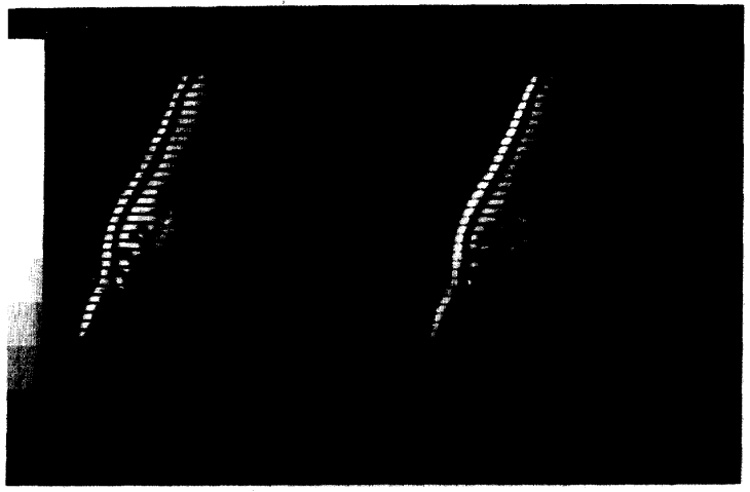
Two of the eight human heart images acquired in a single eight cardiac cycle breath-hold using the segmented k-space CINE-MRI. The dark horizontal lines in these images are the tag lines.

Recently, an automatic tag line detection algorithm has been developed to determine tag locations [6]. In this algorithm, rather than finding the position of an entire tag line in one step, points separated by one pixel along each tag are determined and then these points are connected to define the tag. The search for each point on the tag line is carried out using a least squares fit to a tag profile template. The squared error between the tag template and the profile of the MR image as observed along a line normal to the tag is calculated while shifting the position of the template. The point where minimum error is observed is called the estimate of the tag center (see Fig. 2).

Fig. 2.

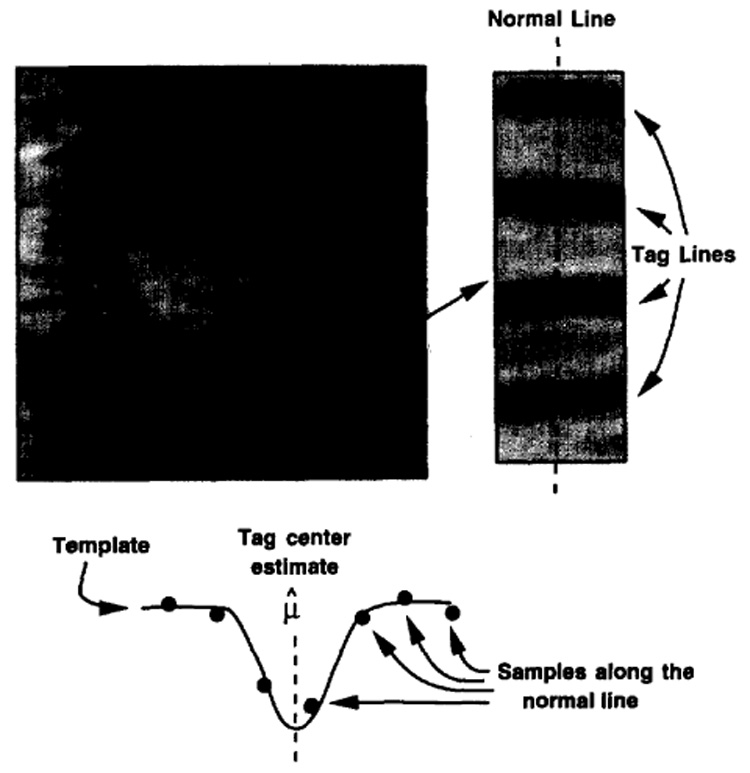
The tag position estimation process. The profile of the image along the normal line is obtained and tag center is estimated using least-squares fitting of the samples along the profile of the template.

It has been shown that the tag line center locations can be found with subpixel accuracy [7]. Accurate tag center estimation leads to accurate measurement of heart wall motion. The main error sources in the estimation of the tag line position are noise and artifacts in the MR images. In this study, we investigated the error sources for tag center estimation and the optimum tag thickness that would minimize this error.

The theory of tag position estimation error is given in the next section. In this section, the effect of the line spread function on the appearance of the tags is discussed, the least squares tag detection algorithm is introduced and then the Cramer-Rao lower bound for the tag position estimation is formulated. Section III concerns the formulation of the optimum tag thickness problem, In this section, in addition to a global expression for the optimum tag thickness, formulation for some important special cases are also given. In Section IV, the theoretical results are verified by Monte-Carlo simulations and phantom experiments.

II. TAG CENTER ESTIMATION ERROR

A. The Tag Generation Method

There are many methods for generating a tag pattern in an MR image. In this paper, the original tag generation pulse sequence used by Zerhouni et. al. [1] was selected as an example (see Fig. 3). Each tagging RF pulse selects a slice perpendicular to the imaging plane. The spoiling gradient applied after the tagging RF pulses causes the spins to lose coherence inside these slices. The intersection between the tag planes created by the tagging RF pulses and the imaging slice appears as dark lines in the images.

Fig. 3.

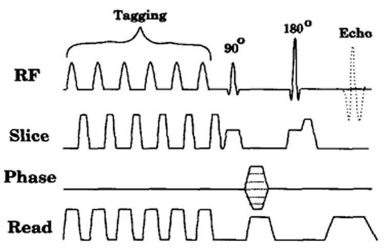
A sample pulse sequence for parallel tag generation. Six RF pulses were applied to generate six parallel tag lines.

By adjusting the RF pulses, the shape and position of the tag line can be changed. The modulation frequency of the RF pulse determines the position of the tag line. The duration and the envelope of the pulse is related to the thickness and the profile of the tag line, respectively.

B. What Do We See in MR Images?

In the MR images, we cannot observe high frequency components of the tag profiles because of the truncation of their Fourier space (k-space) representation. In addition, other factors, such as filtering the MR signal and motion, may change the appearance of the tag. Ignoring the motion artifact changes¹, the tag profile in the image, s(x), can be formulated as the convolution of the original tag profile by the line spread function along the normal direction with the tag line:

$$s\left(x\right)=h\left(x\right)*\text{lsf}\left(x\right)$$ (1)

where s(x) is the tag profile seen in the image, h(x) is the actual tag profile, and "*" is the convolution operator. The line spread function, lsf(x), is the profile seen in the image when the tag line is replaced by an infinitely thin line. In the MR images, samples of s(x) are formulated as:

$$s_i=s(i\Delta x-\mu )+n_{i}i=-\infty ,\dots ,\infty$$ (2)

where s_i are the samples, Δx is the spacing between the samples, and n_i is additive zero-mean white Gaussian noise. The center of the tag is given by the real number µ.

In general, convolution with lsf(x) corresponds to low pass filtering. Depending on $T_2^{*}$, the k-space coverage, and the characteristics of the analog and/or digital filter that may be applied to the MR signal before image reconstruction, the line spread function may change. In the appendix, a sample line spread function is calculated as:

$${\text{lsf}}_{\alpha }\left(x\right)=\frac{1}{\Delta x}\text{sinc}(x/\Delta x)$$ (3)

where

$$\Delta x=\frac{\text{FOV}}{N}\text{max}\left(\right|\text{cos}\alpha |,|\text{sin}\alpha \left|\right)$$

• FOV: Field of view

• N: Number of samples in phase or frequency encoding directions

• α: the angle between the infinitely thin test line and one of the image axes

For this sample analysis, the effect of $T_2^{*}$ on the line spread function is neglected and it is assumed that the MR signal is acquired using an ideal antialiasing filter. No other filtering operation is carried out while reconstructing the image and the image resolution in the phase and frequency encoding directions is the same. The convolution with this sample line spread function corresponds to ideal low-pass filtering.

C. Tag Center Detection Using the Least Squares Error Estimation Method

The center of a tag can be estimated with subpixel accuracy using the least squares estimation (LSE) method. Since the tag generation method is known and the line spread function can be formulated, the expected image of the tag profile, s(x), is obtained using the convolution given in (1). The center of tag, µ, is estimated using LSE by fitting the samples of the tag profile in the image to s(x) (see Fig. 4).

Fig. 4.

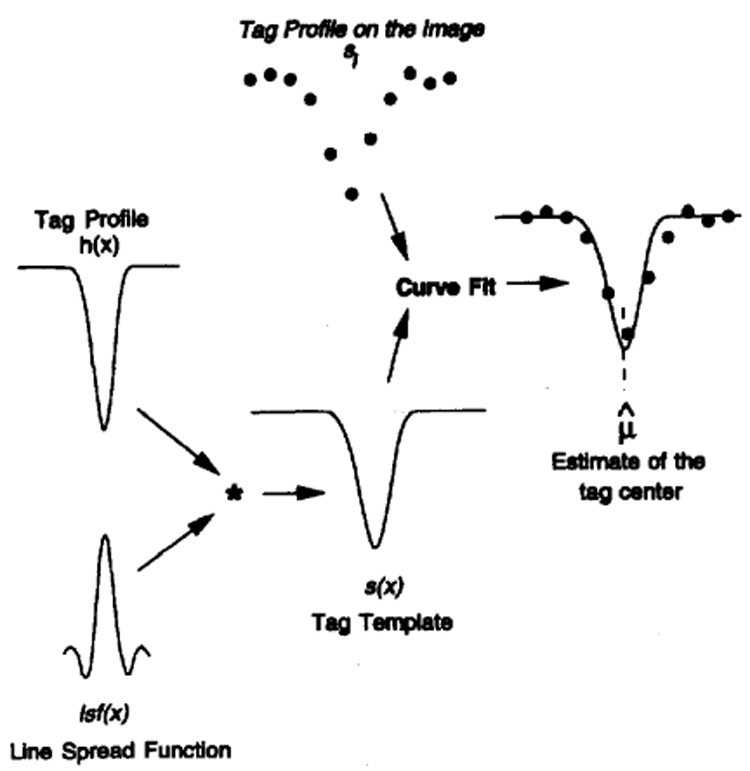
The tag center estimation method. The template is constructed by convolving the tag profile with the line spread function, and the template is fitted to the samples of the tag profile along the normal line.

The LSE method is the best estimation method if the estimation problem is linear. Although the tag center estimation is a nonlinear one, for “reasonable” noise levels the LSE method performs well. What constitutes reasonable noise levels will be explained in Section IVA.

D. Cramer-Rao Bound for the Tag Estimation Error

A lower bound for the tag center estimation error can be derived using the Cramer-Rao bound [8]–[10]. Because the tag center estimation problem is not a linear one, the expected error cannot be found analytically; however, the Cramer-Rao bound for error is tight for “reasonable” noise levels and can be used to determine optimum tag thickness. In the following paragraphs, the bound for the tag estimation error will be derived.

Assume that $\hat{\mu }$ is an unbiased estimate of the tag position, and this value is calculated using the information obtained from the pixels in the MR image. Let {s_i} represent the set of all pixels that will be used to estimate the position of the tag. The Cramer-Rao lower bound is formulated as:

$$E(\hat{\mu }-\mu {)}^2={\sigma }_{\mu }^2\ge -\frac{1}{E\left[\frac{d^2}{{d\mu }^2}lnp\left(\right\{s_i\left\}\right)\right]}$$ (4)

where p({s_i}) is the probability of obtaining the data set, {s_i}, given the position of the tag. In the above equations, E(·) stands for the expected value and σ_µup is the standard deviation of the position estimation error.

The probability of the data set, {s_i}, be can be easily found using the probability of a pixel being at an intensity level given the position of the tag. The probabilistic behavior of the pixel intensity, s_i, is due to the noise. Since the noise is additive, the probability density function (PDF) of the pixel intensity is in the same form as the PDF of the noise:

$$p\left(s_i\right)=\frac{1}{\sqrt{2\pi {\sigma }_n^2}}\text{exp}(-\frac{{(s_i-s(i\Delta x-\mu \left)\right)}^2}{2{\sigma }_n^2})$$ (5)

where ${\sigma }_n^2$ is the variance of the noise. The joint probability density of all the pixels results from the multiplication of the PDF’s of each pixel because the noise on each pixel is independent.

$$p\left(\right\{s_i\left\}\right)=\underset{i=-\infty }{\overset{\infty }{\Pi }}\frac{1}{\sqrt{2\pi {\sigma }_n^2}}\text{exp}(-\frac{{(s_i-s(i\Delta x-\mu \left)\right)}^2}{2{\sigma }_n^2})$$ (6)

Using the above expression and (4) the following result is obtained:

$${\sigma }_{\mu }^2\ge \frac{{\sigma }_n^2}{{\sum }_{i=-\infty }^{\infty }{\left\{\frac{d}{d\mu }s(i\Delta x-\mu )\right\}}^2}$$ (7)

In the above expression, the error bound for the tag position estimation error is calculated using an infinite number of samples. This does not conflict with the limited field of view because the samples that are out of the field of view have a negligible effect on the error bound.

The Cramer-Rao error bound can be written in terms of the line spread function and the tag profile in the Fourier domain. Using Parseval’s theorem, the above relation can be written as:

$${\sigma }_{\mu }^2\ge \frac{2\pi {\sigma }_n^2\Delta x}{\int {\omega }^2{\left|S\right(\omega \left)\right|}^{2}d\omega }$$ (8)

where S(ω) is the Fourier transform of s(x). Since s(x) is a convolution of the tag profile with the line spread function, and convolution corresponds to multiplication in Fourier domain, the following final result can be obtained:

$${\sigma }_{\mu }^2\ge \frac{2\pi {\sigma }_n^2\Delta x}{\int {\omega }^2{\left|H\right(\omega \left)\right|}^2{\left|\text{LSF}\right(\omega \left)\right|}^{2}d\omega }$$ (9)

where H(ω) and LSF(ω) are the Fourier transforms of h(x) (the tag profile) and lsf(x) (the line spread function), respectively.

The above lower bound for the tag center estimation error is tight for “reasonable” noise levels (this will be explained in Section IVA). Therefore, decreasing the lower bound corresponds to decreasing the error. To estimate the tag center precisely, one should decrease the noise level in the image, increase the contrast and the high frequency components of the tag, and increase the image resolution. Although the high frequency components of the tag profile are important for decreasing tag center estimation error, very high frequency components of the tag profile will be suppressed by the low pass filtering effect of the line spread function.

In this section, we derived the Cramer-Rao lower bound for the tag estimation error. In the next section, the optimum tag thickness will be calculated based on this lower bound.

III. OPTIMUM TAG THICKNESS

As discussed in the previous section, the tag center estimation error can be minimized with improved image quality by either increasing the resolution or decreasing the noise on the image. Although a relation between the tag profile and the tag center estimation error is known (see (9)), it is not quite clear which properties of the tag profile are of primary importance for minimizing the estimation error. Here we will analyze the effect of tag thickness on the estimation error.

Let g(x) be a normalized tag profile for which the full-width half max (FWHM) thickness is unity. For the sake of simplicity, let us assume that the normalized tag profile is inverted so that it holds the following relations:

$$\begin{array}{c}g\left(0\right)=1\\ g\left(0.5\right)=g(-0.5)=0.5\\ g(\infty )=g(-\infty )=0\end{array}$$

Thus, the tag profile, h(x), can be written using the normalized tag profile as follows:

$$h\left(x\right)=M_0-C_{t}g\left(\frac{x}{D\Delta x}\right)$$ (10)

where M₀ is the steady state magnetization, C_t is the contrast of the tag, and D is the FWHM tag thickness measured in pixels (see Fig. 5).

Fig. 5.

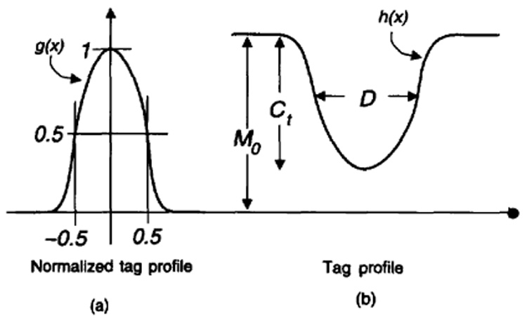
Description of (a) the normalized tag profile and (b) the actual tag profile.

Using the above expression and (9), the following expression for the Cramer-Rao bound is derived:

$${\sigma }_{\mu }^2\ge \frac{{\sigma }_n^2}{C_t^2}\frac{2\pi }{D^2\Delta x\int {\omega }^2{\left|G\right(D\Delta x\omega \left)\right|}^2{\left|\text{LSF}\right(\omega \left)\right|}^{2}d\omega }$$ (11)

where G(ω) is the Fourier transform of the normalized tag profile, g(x). In the above expression, M₀ does not appear because it does not contain any information about the tag position.

It is interesting to observe that the error bound is inversely proportional to the contrast to noise ratio (CNR). To simplify the notation a new variable, the “error factor”, is introduced. It is basically the multiplication of the CNR by the estimation error:

$$\Gamma =\frac{C_t}{{\sigma }_n}\frac{{\sigma }_{\mu }}{\Delta x}$$ (12)

In this expression, the estimation error is divided by the pixel dimension, Δx, so that the unit of Γ is pixels. For example, if the estimation error factor, Γ, is equal to one pixel, then the estimation error becomes 1/CNR pixels. It is important to note that choosing the tag thickness to minimize Γ will also minimize σ_µ.

If (11) and (12) are combined, the following inequality for the error factor can be obtained:

$${\Gamma }^2\left(D\right)\ge \frac{2\pi D}{\int {\omega }^2{\left|G\right(\omega \left)\right|}^2{\left|\text{LSF}(\frac{\omega }{D\Delta x})\right|}^{2}d\omega }$$ (13)

Since it is based on the Cramer-Rao bound, the above lower bound is also tight.

For cases where the above inequality turns into an quality (when the noise level is low), it is possible to obtain the optimum tag thickness. One method is to plot the curve of error factor versus tag thickness and then find the minimum point on this curve. As an example, Fig. 6(b) shows the curves of error factor versus tag thickness for the normalized tag profiles shown in Fig. 6(a). In this figure, g1(x) and g4(x) correspond to Gaussian and rectangular tag profiles. g2(x) and g3(x) are the normalized profiles of the tags that are generated using the pulse sequence shown in Fig. 3. All the RF pulses are sinc function multiplied by Hamming window. For generation of g2(x) only the main lobe of the sinc is used, while for g3(x) one side lobe is added to the RF pulse. The curves shown in Fig. 6 are obtained assuming a sinc point spread function and vertical or horizontal line tag placement. The optimum tag thickness ranges from 1.13 for the Gaussian to 1.50 pixels for the rectangular tag profiles. Table I shows the optimum tag thickness values and the error factor at these optimum values. The tag center estimation errors for a CNR value of 20 are also shown. If the resolution of an image in readout and phase encoding directions are the same, diagonal placement of tag lines will give the best result because in the diagonal direction the width of the line spread function is narrower than all the directions (see appendix). If the tag lines are placed diagonally, all the values in Table I will be divided by 1.41. In this case, the optimum thickness ranges from 0.80 to 1.06 pixels.

Fig. 6.

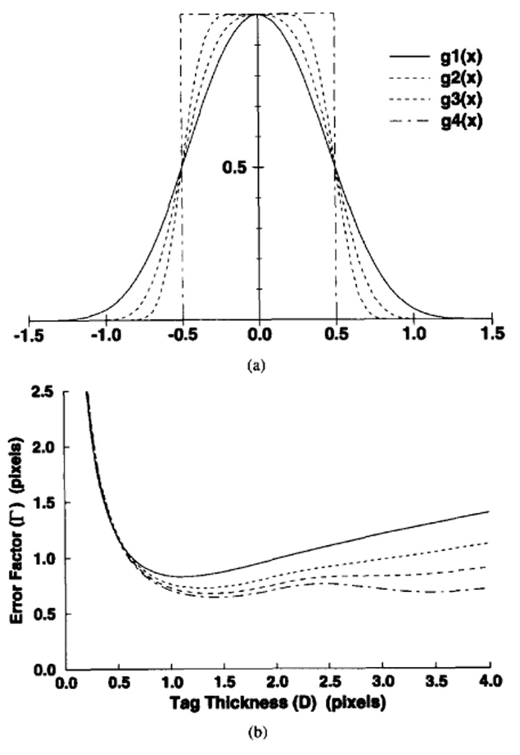
Sample normalized tag profiles, g(x) and error factor, Γ, curves. For these sample plots, the line spread function is assumed to be sinc as in (3). The tag profiles are given in (a), corresponding error factors curves are given in (b)‥ g1(x) and g4(x) are the Gaussian and rectangular tag profiles, respectively.

TABLE I.

The optimum tag thicknesses for the sample tag profiles in Fig. 6. The error factor, Γ, for optimum tag thickness is also given. The tag center estimation error is calculated for a CNR value of 20.

Normalized Tag Profile	Optimum Tag Thickness Dopt (pixels)	Minimum Error Factor Γmin (pixels)	Tag Center Estimation Error for CNR=20 σµ (pixels)
g1(x)	1.13	0.82	0.041
g2(x)	1.35	0.73	0.037
g3(x)	1.40	0.65	0.033
g4(x)	1.50	0.62	0.031

The error factor versus tag thickness graphs have very similar characteristics. They are smooth, have a single minimum, and as the tag thickness goes to infinity or zero, the error factor goes to infinity. The error factor for tag thicknesses less than the optimum value can be approximated by the tangent line for D → 0 as:

$${\Gamma }_0^2\left(D\right)=\frac{2\pi }{D^2{\left|G\right(0\left)\right|}^2\int {\omega }^2{|\text{LSF}(\omega /\Delta x)|}^{2}d\omega }$$ (14)

Similarly, the error factor for tag thicknesses higher than the optimum value can be approximated by the tangent line for D → ∞ as:

$${\Gamma }_{\infty }^2\left(D\right)=\frac{2\pi D}{{\left|\text{LSF}\right(0\left)\right|}^2\int {\omega }^2{\left|G(\omega )\right|}^{2}d\omega }$$ (15)

The intersection point of these curves gives an approximate value for the optimum tag thickness as (see Fig. 7):

$$D_{\text{opt}}^3\approx \frac{{\left|\text{LSF}\right(0\left)\right|}^2}{\int {\omega }^2{\left|\text{LSF}\right(\omega /\Delta x\left)\right|}^{2}d\omega }·\frac{\int {\omega }^2{\left|G\right(\omega \left)\right|}^{2}d\omega }{{\left|G\right(0\left)\right|}^2}$$ (16)

At this optimum value, the tag center estimation error can be approximately calculated using (14) (or (15)) and (16) as:

$${\sigma }_{\mu }^2\approx \left(\frac{{\sigma }_n^2}{C_t^2}\right)·2\pi {\left(\Delta x\right)}^2/\left\{{\left|G\left(0\right)\right|}^{2/3}{\left(\int {\omega }^2{\left|G\left(\omega \right)\right|}^{2}d\omega \right)}^{2/3}{\left|LSF\left(0\right)\right|}^{4/3}{\left(\int {\omega }^2{\left|LSF\left(\omega /\Delta x\right)\right|}^{2}d\omega \right)}^{1/3}\right\}$$ (17)

As seen from the above approximate expression, to decrease the tag center estimation error, one should increase the high frequency components of the tag profile, corresponding to a more rectangular profile. The longer RF pulses required to obtain a more rectangular tag profile, however, may not be optimal because the decrease in the tag center estimation error is small. As the profile approaches a rectangular, the optimum thickness increases from a value of 1.13 to 1.50 pixels and the center estimation error factor decreases from a value of 0.82 to 0.62 pixels (see Fig. 6 and Table I).

Fig. 7.

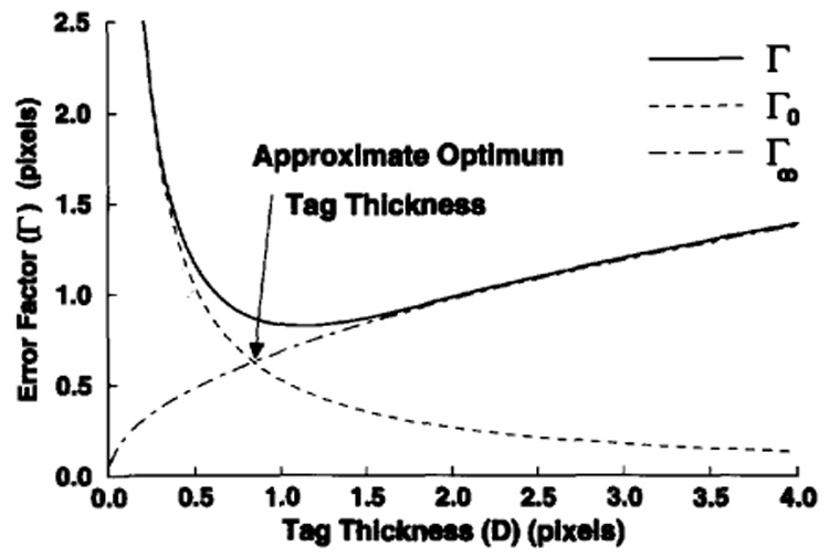
A sample error factor curve. For this example, it is assumed that the point spread function is sinc and the tag profile is Gaussian.

The other factor affecting tag center estimation error is the line spread function. As the high frequency components of the line spread function increase, the error decreases. Here, the limitation for increasing the high frequency components of the line spread function is the imaging method itself. The truncation of the k-space data is an important factor. Truncation causes a sinc-type point spread function. All the other possible sources that may affect the point spread function broaden the sinc. Thus, by increasing the imaging quality, tag center estimation error can be decreased.

The tag center estimation is proportional to the pixel separation. At first glance one might think that decreasing the pixel separation (increasing the image resolution) would decrease the estimation error. However, decreasing the pixel separation results in a diminished contrast to noise ratio that is inversely proportional to the error. Therefore, increasing the image resolution may not decrease the tag center estimation error.

In this section, we derived a simple relation between tag thickness and the error factor, and calculated an approximate expression for the optimum tag thickness and the tag center estimation error at this optimum value. In the following section, the above results were verified using Monte-Carlo simulations and experiments.

IV. SIMULATIONS AND EXPERIMENTS

A. Simulations

The Cramer-Rao bound may not be tight if the contrast to noise ratio is low. Conversely, the optimum tag thickness is derived assuming the error factor is approximately equal to its lower bound. So the derivation may fall below a CNR threshold. To find this threshold, the error factor is calculated for different noise levels and tag thicknesses using Monte-Carlo simulations, and compared to the lower bound.

The block diagram showing the method of obtaining the value of Γ for a given noise level is depicted in Fig. 8. Here, a Gaussian tag profile and sinc line spread function is assumed. The noise is generated using a Gaussian noise generation program [11, pp. 216–217]. For each point on the Γ curve, 1,000 data sets are generated and the position of the tag is estimated using LSE for each data set. The standard deviation of all the estimations is approximately equal to σ_µ. The value of Γ is obtained using (12). This process is carried out for five different noise levels and eighteen different tag thicknesses.

Fig. 8.

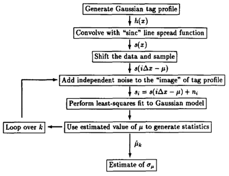
The block diagram for Monte-Carlo simulations.

Fig 9. shows the results of this process as well as the theoretical lower bound for Γ. As seen from the figure, if CNR is greater than 10, then the error factor is very close to the lower bound. For low CNR values (less than 10), the Γ curve is above the lower bound curve. For CNR levels of 5, the optimum tag thickness becomes higher than the calculated optimum thickness value, and the error factor, Γ, at this point, is 15% more than the minimum value of the error factor lower bound. For all practical purposes this increase is acceptable. However, for even lower CNR values, the tag is barely visible, and the LSE method finds the noise-generated local minima at arbitrary locations.

Fig. 9.

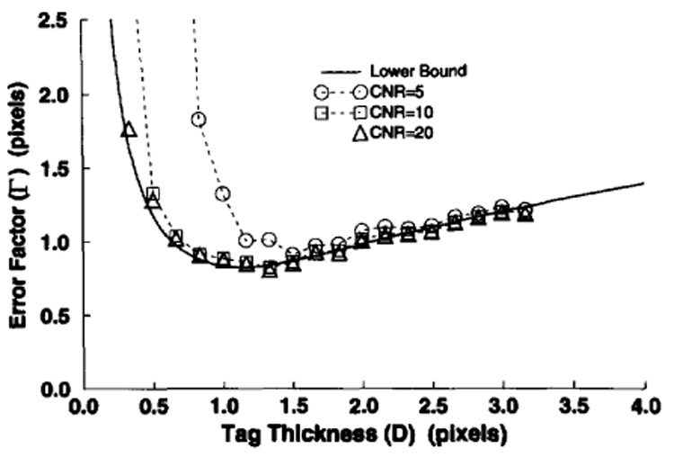
The results of the Monte-Carlo simulations. Points are calculated using five different levels of CNR. The lower bound for Γ is also given.

As a result, the error factor is approximately equal to its lower bound if contrast to noise ratio is higher than 10. Conversely, for CNR < 5, the LSE algorithm fails to detect thin tag lines, and therefore the actual optimum tag thickness doesn’t match with the calculated optimum tag thickness.

B. Experiments

We designed a set of experiments to verify the theoretical relation between the tag center estimation error and the tag thickness. In these experiments, tag thickness was varied while keeping the other imaging parameters constant. Using the data in the images, experimental values for the error factor were obtained for different tag thicknesses.

The pulse sequence used in the experiments is shown in Fig. 3. The pulse sequence was designed to generate six parallel tag lines per MR image. The envelope of the tagging RF pulses has only the main lobe of the sinc pulse multiplied by a Hamming function, generating tag profiles very similar to Gaussian.

A uniform spherical phantom was placed in the region of interest. All the filters in the vendor-supplied reconstruction program that could change the noise characteristics and affect line spread function were turned off. A total of 13 images were acquired. The field of view and size of these images were 16 cm and 256 × 256, respectively. The pixel separation was therefore Δx = 0.625 mm. The tag thickness was varied by changing the strength of the tagging gradient. The duration of the tagging RF pulses was kept fixed at 9.6 msec for the first six images (for tag thicknesses 0.67, 0.83, 1.00, 1.33, 2.66, and 5.32 pixels) while the duration was 6.4 msec for the last seven images (for tag thicknesses 1.0, 1.33, 1.67, 2.00, 2.50, 5.00 and 8.00 pixels). Four of these images and their horizontal profiles are shown in Fig. 10.

Fig. 10.

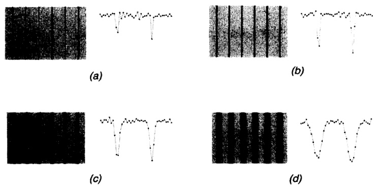
Four of the 13 phantom images used in these experiments. There were six parallel tag lines in each image. The tag thicknesses are: (a) 0.67, (b) 1.33, (c) 2.66, and (d) 5.33 pixels. On the right-hand side, a sample profile of each image is shown.

Due to the RF field inhomogeneity and different amount of T₁ relaxation [12], the intensity variation in the images was observed. At the center of each image, the CNR for the tags was relatively constant. The 128 horizontal profiles from the center part of the image were analyzed independently. On each profile, six tag positions were estimated using the LSE algorithm.

An estimate for σ_µ was obtained from the analysis of each tag line from 128 µ estimations along the tag. Since the phantom was stationary and uniform, the tag lines were expected to be subject to bending because of field inhomogeneity [13, 14]. A second-order curve was fitted to the set of µ estimations. The standard deviation of the estimates from the second-order curve was equal to the standard deviation of µ within the 15% error margin predicted by the statistics of the 128 samples.

To calculate the CNR of a tag, the noise level and amplitude of the tag was calculated. To measure the noise level, the phantom was taken out from the MR scanner, and a blank image was acquired while keeping all other imaging parameters constant. The noise level, σ_n, results from dividing the standard deviation of the pixel intensities in the image by 0.655 (see [15], for the relation between the background noise level and the noise level in the image). The amplitude of each tag was calculated in two steps. First, a phantom image with no tag was acquired. A second order function was fitted to the intensity distribution in the image. M₀ values at the position of each tag were calculated using this function. Second, the minimum signal intensity along the tag profile was measured. To eliminate the effect of the point spread function, thick tag lines were selected. The average of the minimum values along the tag line gave an estimate for the minimum signal intensity on the tag profile. Subtracting this value from the calculated M₀ gives the contrast of the tag, C_t. The ratio between the contrast and the noise level gives the CNR of the tag.

Using the estimated values of CNR and the tag center estimation error, the error factor, Γ, was calculated using equation (12) for each tag line in each phantom image. In Fig. 11, the experimentally evaluated error factor values are plotted on a Γ versus D curve. On the same graph the lower bound for the error factor is also given. As seen in the graph, the experimental values for the error factor are very close to the lower bound curve. The deviation is within the 15% experimental error boundaries determined by the 128 samples. However, there seems to be a small systematic error between the theoretical lower bound and experimental results for D values less than the optimum. It is known that for D < D_opt, the value of Γ depends on the line spread function rather than the tag profile. In the theoretical calculations of the error factor, the line spread function was assumed to be sinc. If one considers the effect of $T_2^{*}$ decay, however, the line spread function may be calculated more accurately and this may account for this small systematic error.

Fig. 11.

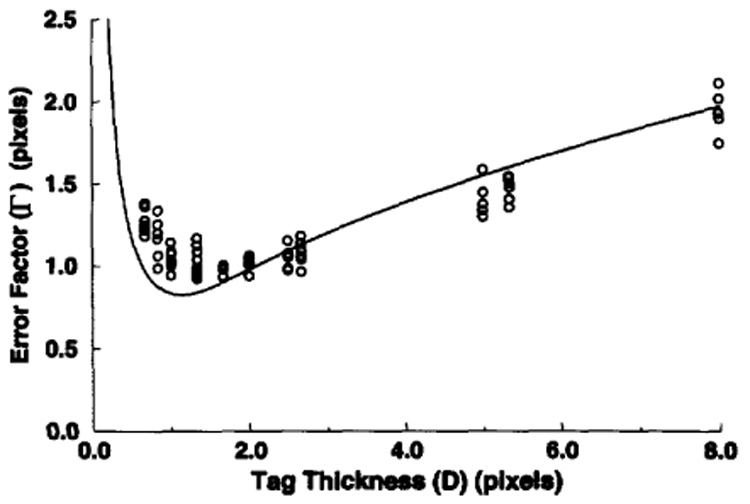
Experimental measurement results of the error factor (Γ) for different tag thicknesses. Each circular symbol corresponds to an estimate of the error factor from 128 profiles on a single tag line. The calculations are carried out for 13 images with six tag lines on each. The lower bound for the error factor is shown as a solid line.

V. CONCLUSION

We analyzed the precision of the magnetic resonance tag detection [6], [12] and have shown that the tag position can be estimated with subpixel accuracy, and that the estimation error depends on tag thickness. An approximate expression for the optimum tag thickness has been derived. The result was verified using Monte-Carlo simulations and experiments.

Depending on the angle and the shape of the tag line, the optimum tag thickness is in the range of 0.8 to 1.5 pixels. If optimum tag thickness is used, the tag position can be estimated with an error less than 0.9/CNR pixels, leading to the following conclusions:

• Tag position estimation error increases drastically as tag thickness decreases for values less than the optimum. For tag thicknesses higher than the optimum, however, a small increase in error is observed.

• Tag position estimation error and optimum tag thickness are both dependent on the shape of the tag profile. As the tag profile becomes closer to a rectangular shape, the optimum tag thickness increases and the estimation error decreases. There is little to be gained by designing RF pulses that give the “optimum tag profile.”

• The optimum tag thickness is also dependent on the orientation of the tag line because the line spread function is angle-dependent. For example, if the resolution in phase and frequency encoding directions are the same, the resolution along the diagonal directions becomes maximum. In this case, the tag thickness and the tag center estimation error can be decreased by placing the tag line diagonally.

• The optimum tag thickness is independent of the contrast to noise level. However, the tag position estimation error is linearly proportional to the noise level. As was discussed in Section IVA, this statement is not valid for CNR levels lower than 10. At low CNR values, the optimum tag thickness increases as CNR decreases.

Following are guidelines for the use of the cardiac tagging technique:

• Use a tag thickness slightly higher than the optimum thickness (for example 2 pixels wide) to avoid the tag thickness becoming less than optimum during the later phases of the cardiac cycle.

• Avoid long tag generation pulses because the shape of the tag line is not critical.

• Place the tag lines perpendicular to the highest resolution direction.

To obtain high accuracy strain field, tag spacing should be as close as possible. However, the tag center estimation may be affected by the Gibbs ringing of the neighboring tag lines. In tag center estimation, the tag separation is assumed to be high so that this effect is negligible. Because the optimum tag thickness is on the order of one pixel, close tag spacing is possible. The combination of lower tag spacing and high precision tag position estimation leads to accurate measurement of strain fields. The analysis of the Gibbs ringing and the problem of finding the optimum tag spacing is currently being studied.

In this study, the data acquisition method is assumed to be arranged so that the effect of motion on image quality is negligible. However, it is known that motion causes blurring in MR images and the blurring is dependent on the direction of the motion. Since blurring affects the line spread function, the optimum tag thickness and the estimation error are also affected. To find the optimum thickness for the images where blurring due to motion is present, both theoretical and experimental studies are necessary.

APPENDIX

LINE SPREAD FUNCTION

In this appendix, we will concentrate on imaging a line whose profile is an impulse and derive an analytical expression for a sample line spread function. Several factors, such as truncation of the k-space data, $T_2^{*}$ decay, and filters used during data acquisition and image reconstruction steps affect image quality with MRI. In the calculation of the line spread function, however, $T_2^{*}$ decay is ignored and it is assumed that the data acquisition is carried out using an ideal antialiasing low pass filter and that no other filters are used. Thus, we assumed that the only factor affecting image quality is the truncation.

The line spread function is the profile of a line image along the normal direction, as opposed to the point spread function, which is the image of a point. It is known that because of the truncation of k-space data, a point appears as a sinc function on an MR image. Assume that the imaging resolution in the phase and frequency encoding directions are the same (N × N). Under this condition, the point spread function can be written as:

$$\text{psf}(x,y)=\frac{N^2}{{\text{FOV}}^2}\text{sinc}\left(\frac{Nx}{\text{FOV}}\right)\text{sinc}\left(\frac{Ny}{\text{FOV}}\right)$$ (18)

where FOV stands for the field of view. Using the point spread function, it is possible to calculate the image of any function. This represents the two dimensional convolution of the function with the point spread function.

To calculate the image of the line, let us define the line as:

$$l(x,y)=\delta (x\text{cos}\alpha +y\text{cos}\alpha )$$ (19)

where δ(x) is the Dirac delta function and α is the angle of the line. The resulting line image, I, is the convolution of the line with the point spread function, which can be calculated as:

$$\begin{array}{ccc}I(x,y)& =& l(x,y)**\text{psf}(x,y)\\ & =& \frac{1}{\Delta x}\text{sinc}\left(\frac{x\cos \alpha +y\sin \alpha }{\Delta x}\right)\end{array}$$ (20)

where Δx = FOV/N max(|cos α|, |sin α|).

The line spread function represents the function of the image along the normal direction as it relates to the imaged line. It can be written as

$${\text{lsf}}_{\alpha }\left(x\right)=I(x\text{cos}\alpha ,x\text{sin}\alpha )$$ (21)

Using the above two equations, and redefining α as the angle between the line and either the x or y axis, whichever is closer, one can obtain the following simple relation for the line spread function:

$${\text{lsf}}_{\alpha }\left(x\right)=\frac{1}{\Delta x}\text{sinc}\left(\frac{x}{\Delta x}\right)$$ (22)

Thus, even for an image with equal resolution in the phase encoding and frequency encoding directions, the line spread function depends on the line direction. In our example, the function is sinc and its frequency changes according to the angle of the line. The maximum frequency is obtained when the line is diagonal, or equivalently, the maximum resolution is along the diagonal direction.

REFERENCES

- 1.Zerhouni EA, Parish DM, Rogers WJ, Yang A, Sapiro EP. Human heart: tagging with MR imaging—a method for noninvasive assessment of myocardial motion. Radiology. 1988;169:59–63. doi: 10.1148/radiology.169.1.3420283. [DOI] [PubMed] [Google Scholar]
- 2.Axel L, Dougherty L. MR imaging of motion with spatial modulation of magnetization. Radiology. 1989;171:841–845. doi: 10.1148/radiology.171.3.2717762. [DOI] [PubMed] [Google Scholar]
- 3.McVeigh ER, Atalar E. Cardiac tagging with breath hold CINE MRI. Magn. Reson. Med. 1992;28:318–327. doi: 10.1002/mrm.1910280214. [DOI] [PMC free article] [PubMed] [Google Scholar]
- 4.Yun KL, Niczyporuk MA, Daughters D, T G, Ingels J, Stinson EB, Alderman EL, Hansen DE, Miller DC. Alterations in left ventricular diastolic twist mechanics during acute human cardiac allograft rejection. Circ. 1991;83:962–973. doi: 10.1161/01.cir.83.3.962. [DOI] [PubMed] [Google Scholar]
- 5.Bolster BD, Jr, McVeigh ER, Zerhouni EA. Myocardial tagging in polar coordinates with use of striped tags. Radiology. 1990;177:769–772. doi: 10.1148/radiology.177.3.2243987. [DOI] [PMC free article] [PubMed] [Google Scholar]
- 6.Guttman MA, Prince JL, McVeigh ER. Tag and contour detection in tagged MR images of the left ventricle. IEEE Trans. on Medical Imaging. 1994 Mar.13 doi: 10.1109/42.276146. [DOI] [PubMed] [Google Scholar]
- 7.McVeigh ER, Zerhouni EA. Noninvasive measurement of transmural gradients in myocardial strain with magnetic resonance imaging. Radiology. 1991;180:677–683. doi: 10.1148/radiology.180.3.1871278. [DOI] [PMC free article] [PubMed] [Google Scholar]
- 8.Ljung L, Soederstroem T. Theory and Practice of Recursive Identification. London: The MIT Press; 1983. [Google Scholar]
- 9.Komo JJ. Random Signal Analysis in Engineering Systems. London, UK: Academic Press; 1987. [Google Scholar]
- 10.Sandell NR, Jr, Shapiro JH. Lecture Notes. Dept. of Elect. Eng. and Comput. Sci., Massachusetts Inst. of Technol.; 1976. Stochastic processes and applications. [Google Scholar]
- 11.Press WH, Flannery BP, Teukolsky SA, Vetterling WT. Numerical Recipes in C: The Art of Scientific Computing. Boston, MA: Cambridge University Press; 1988. [Google Scholar]
- 12.McVeigh ER, Yang A, Zerhouni EA. Measurement of T1 with spatially selective pre-inversion pulses. Med. Phys. 1990;17:131–134. doi: 10.1118/1.596543. [DOI] [PMC free article] [PubMed] [Google Scholar]
- 13.McVeigh ER, Zerhouni EA. Measuring gradient performance with presaturation stripes. Radiology. 1989;173(P):227. [Google Scholar]
- 14.Mosher TJ, Smith MB. Magnetic susceptibility measurement using a double-dante tagging (ddt) sequence. Magn. Reson. Med. 1991 Mar.18:251–255. doi: 10.1002/mrm.1910180127. [DOI] [PubMed] [Google Scholar]
- 15.Henkelman RM. Measurement of signal intensities in the presence of noise in [MR] images. Med. Phys. 1985 Mar.-Apr.12:232–233. doi: 10.1118/1.595711. [DOI] [PubMed] [Google Scholar]