Improved mapping of information distribution across the cortical surface with the Support Vector Machine

Abstract

The early visual cortices represent information of several stimulus attributes, such as orientation and color. To understand the coding mechanisms of these attributes in the brain, and the functional organization of the early visual cortices, it is necessary to determine whether different attributes are represented by different compartments within each cortex. Previous studies addressing this question have focused on the information encoded by the response amplitude of individual neurons or cortical columns, and have reached conflicting conclusions. Given the correlated variability in response amplitude across neighboring columns, it is likely that the spatial pattern of responses across these columns encodes the attribute information more reliably than the response amplitude does. Here we present a new method of mapping the spatial distribution of information that is encoded by both the response amplitude and spatial pattern. This new method is based on a statistical learning approach, the Support Vector Machine (SVM). Application of this new method to our optical imaging data suggests that information about stimulus orientation and color are distributed differently in the striate cortex, and this observation is consistent with the hypothesis of segregated representations of orientation and color in this area. We also demonstrate that SVM can be used to extract ‘single-condition’ activation maps from noisy images of intrinsic optical signals.

Introduction

The early visual cortices, including the striate cortex (V1), represent information of several stimulus attributes, such as orientation and color (Hubel and Wiesel, 1968; Gouras, 1970). To understand the coding mechanism of these attributes in the brain, and the functional organization of these cortices, it is necessary to establish whether different attributes are represented by separate anatomical compartments in each cortex. In other words, is each cortex one general-purpose network that represents various attributes, or does it consist of several specialized networks, each representing a single specific attributes?

In the past two decades, this important question has been studied by several groups, but it is still controversial. An influential study by Livingstone and Hubel (1984) reported that the cytochrome oxidase (CO) rich blobs in V1 and the regions between them (interblobs) contain distinct and segregated populations of neurons that differ in their selectivity for color or orientation. This study suggested that blobs and interblobs in V1 are specialized compartments for processing color and orientation information, respectively. This hypothesis of color/orientation segregation in V1 was supported by some subsequent studies (e.g., Ts’o and Gilbert, 1988; Yoshioka and Dow, 1996), but challenged by others (e.g., Lennie et al., 1990; Leventhal et al., 1995).

Because these previous studies investigated the amplitude of the responses of cortical neurons to various stimuli, their conclusions were based on the distribution of information that is encoded by the response amplitude. Given the variability of neuronal response to any given stimulus (Schiller et al., 1976; Dean, 1981; Snowden et al., 1992; Kara et al., 2000; Gur and Snodderly, 2006), a coding scheme based on response amplitude of individual neurons is likely unreliable. Moreover, the variability of neuronal activities is correlated over a cortical distance that is as large as 1 mm cross (Arieli et al., 1996). Because of this correlation, a coding scheme that is based on the averaged response amplitude of individual columns is also unreliable. In contrast, spatial patterns of the response across a small region might be less affected by the correlated variability, and thus encode stimulus information more reliably than do response amplitudes alone. This hypothesis is supported by our recent findings that stimulus color and luminance are encoded by the peak locations of response patches in areas V1 and V2 (Xiao et al., 2003; Wang et al., 2007; Xiao et al., 2007a).

However, although the spatial patterns of cortical activities can be mapped by modern imaging techniques, there has been no method to map the distribution of information that is encoded by these spatial patterns. Here we introduce such a method, which is based on a recently developed learning machine called the Support Vector Machine (SVM) (Vapnik, 1998). This method can be used to determine whether information about different stimulus attributes such as color and orientation is represented in different compartments of visual cortices. A brief summary of the advantages of the SVM method over previous methods is given in the METHODS section. The description of an application of this method has been published previously (Xiao et al., 2007b). The current paper provides a more detailed description of the method itself, along with its other applications.

Methods

Experiments were carried out on two anesthetized and paralyzed monkeys (Macaca fascicularis). Details of the methods have been described in previous publications (Xiao et al., 2007a; Xiao et al., 2007b). Here we describe only the methods that are essential for understanding the current paper.

Optical imaging

We recorded intrinsic optical signal with a CCD camera with 652 × 492 pixels. The camera took 10 frames/second at a resolution of 6.1 μm/pixel in color experiments, or 12.2 μm/pixel in orientation experiments. The cortex was illuminated by 610 (±8) nm light from LEDs driven by a stabilized power supply.

During each imaging trial, 11 frames were taken before, 30 or 18 during, and 2 after the 3 or 1.8 second presentation of a stimulus, followed by a rest period of 11–13 seconds, during which the display was uniformly gray (Fig. 1). An imaging block consisted of one imaging trial for each stimulus, including a control trial without stimulation, presented in a pseudorandom order. Each functional map was derived from an experiment consisting of 50–51 imaging blocks.

Figure 1.

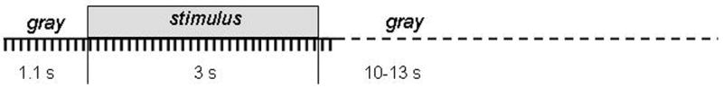
A schematic depiction of the experimental protocol, showing the temporal sequence of stimulus presentation and data acquisition. Each tick mark indicates the time at which a cortical image was acquired. In some experiments, each stimulus was presented for 1.8 seconds instead of 3 seconds, and 18 images instead of 30 ones were taken during the stimulus presentation.

For each imaging trial, we calculated the average of 11 pre-stimulation frames and the average of the last 7 frames (5 during-stimulation frames and 2 after-stimulation ones). Subtracting the former from the latter produced an activation map for the given trial, in which darker pixels indicate higher neural activity. Each activation map was then filtered by a band-pass filter (Difference of Gaussian (DOG) with σ₁ = 12.2 μm for color-related data, or 24.4 μm for orientation-related data; σ₂ = 331.8 μm for all data), to remove both high frequency noise and very low frequency gradients. This filter also reduced the global intrinsic signal that is not specific to the stimulus [8]. The filtered single-trial activation maps were used in the subsequent analyses.

The SVM classifier

Advantages of the SVM method over previous methods of image analysis

1. Does not rely on response amplitude alone, which is notoriously variable and unreliable

2. Takes advantage of correlations between responses in several pixels, and thus exploits the spatial pattern of activity across the image

3. Automatically rejects outliers, which are often due to artifacts from blood vessels or uneven illumination

4. Can be used to map the distribution of information about a specific stimulus attribute such as color or orientation across the imaged area.

5. Unlike linear discriminant analysis, SVM makes no assumptions about the distribution of the signal or the noise.

Calculation procedure

For the purpose of illustration, we discuss vectors of 2 elements in this section. In our real application, each vector represents an image, and each vector element represents an image pixel. Fig. 2 shows two groups of vectors. Each axis represents the value of one element. We use a variable c_i to denote the group to which the vector X_i belongs. Each c_i has a value of either 1 or −1. A linear SVM classifier derives a dividing hyperplane (the solid line in Fig. 2) in the form of W·X−b = 0. Each of the dashed lines that are parallel to the hyperplane passes at least one element from one group, and there are no elements between these two dashed lines. The SVM classification algorithm searches for a specific hyperplane with associated parallel hyperplanes (the dashed lines) that are maximally separated.

Figure 2.

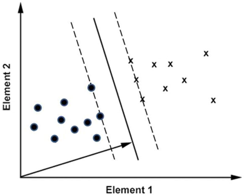
SVM classification of two-dimensional vectors. Two groups of vectors are represented by label “X” and circle, respectively. The solid line represents the hyperplane of the SVM classifier. The arrow represents the direction of the weight vector associated with the hyperplane.

The weight vector W is orthogonal to the hyperplane, as represented by the arrow in Fig. 2, and has a length of 2/d, where d is the distance between the two dashed lines. Therefore W is derived by the following optimization:

min(||W||²/2) subject to the condition that

c_i(W·X_i − b) >=1 and 1 <= i <= n, where n is the total number of vectors.

This algorithm applies to cases where the two groups can be completely separated by a hyperplane. Such cases are called linearly separable.

If the two groups are not linearly separable, the weight vector W is derived by the following optimization:

$min(\frac{1}{2}|\left|W\right|{|}^2+{\displaystyle \sum _i}{\xi }_i)$ subject to the condition that

$${\text{c}}_{\text{i}}(W·{\text{X}}_{\text{i}}-\text{b})>=1-{\xi }_i,\hspace{0.17em}1<=\text{i}<=\text{n},\hspace{0.17em}\text{and\hspace{0.17em}}{\xi }_i>=0.$$

Our SVM classification was implemented with a Matlab program provided by C-C. Chang and C-J. Lin (LIBSVM: a library for support vector machines, 2001; Available at http://www.csie.ntu.edu.tw/~cjlin/libsvm/).

The above algorithm classifies two classes of vectors, and is called a two-class classifier. To classify N classes of vectors, a total of N(N−1)/2 two-class classifiers are built, each for one of the possible pairs of classes. With these two-class classifiers, we can determine to which class a test vector belongs by the following procedure. First, the test vector will be classified by one of the two-class classifiers. This classifier will determine which of the two classes is likely to contain the test vector, and give that class a vote. Second, the above step is repeated for each of the N(N−1)/2 two-class classifiers. The class that gets the most votes during the entire procedure is taken as the one that the test vector belongs.

Vector summation for orientation maps

In the experiment on orientation representation, all single-trial activation maps (after multiplying their angles by two) were added vectorially on a pixel-by-pixel basis (Bonhoeffer and Grinvald, 1991). The resulting vector angles (divided by two) formed an orientation preference map, and the map of vector lengths formed an orientation selectivity map.

Results

SVM-derived relative information map

In one experiment, we imaged the responses of cortical areas V1 and V2 to achromatic gratings of 6 different orientations that were evenly distributed between 0 and 180 degrees. Each orientation was presented 50 times and was thus associated with 50 single-trial activation maps. The averaged activation maps for 0° and 90° stimuli are shown in Figs. 2A and 2B, respectively. Before determining the distribution of orientation information across the imaged cortical region, we need to determine whether the response patterns across this region carried information about stimulus orientation. For this purpose, we tested whether the stimulus orientation can be deduced from its associated single-trial activation map. This was done by combining the SVM classification algorithm with a procedure of cross validation in the following sequence. First, we trained a linear SVM classifier with the single-trial activation maps derived from 49 imaging blocks. Then, we used the classifier to determine the stimulus orientation from each single-trial activation map that was derived from the remaining (50^th) block. Finally, we repeated the above procedure 50 times, each time using a different block in the step of orientation deduction. We found that the stimulus orientations were deduced correctly from 99.7% single-trial activation maps, which is much higher than the chance accuracy (16.7%) that would have been obtained if the single-trial activation maps carried no orientation information. This high accuracy suggests that each single-trial activation map contained enough information for discriminating the 6 stimulus orientations used in this experiment. It also suggests that the orientation information in our response images can be reliably extracted by the linear SVM algorithm.

To determine how the orientation information was distributed across the imaged region, we assessed the relative contribution that each pixel made to the successful SVM classification. The weights vector associated with an SVM classifier can be used to map these relative contributions, as suggested by an examination of the weight vector and its relation to each element’s contribution to the classification shown in Fig. 2.

In Fig. 2, the direction of the weight vector W is represented by the arrow. It is clear that the two groups of vectors are more easily discriminated when only element 1 is used, compared to when only element 2 is used. Correspondingly, the projection of W on the axis representing element 1 is greater than the projection on the axis representing element 2. Therefore, the projection of W on the two axes can be used to assess the relative contributions of these two elements to the classification. In our application, each vector represents an image, and each element represents a pixel.

When N groups of images need to be classified, a total of N(N−1)/2 two-class SVM classifiers are built, one for each possible pair of groups. Each two-class classifier is associated with a weight vector (W_j, j = 1, …, N(N−1)/2 ). The contribution of the ith pixel to the entire process of classification is measured by $K_i=\sqrt{{\displaystyle \sum _j}{W}_{ji}^2}$, where W_ji denotes the projection of W_j on the ith pixel. We call the image consisting of K_i the relative information map, because a pixel with a greater K_i makes a greater contribution to the classification, and thus carries more information about the identity of the stimulus that gave rise to each image. Since each two-class classifier plays an equal role in the process of classification, it should contribute equally to the calculation of the information map. To ensure this, each weight vector (W_j) is normalized to have a length of 1 before being used in the above calculation.

Fig. 3C shows the relative information map about orientation for the experiment described above. It was derived from the SVM classification over the entire data set of 50 imaging blocks. This figure shows that the information about stimulus orientation is not distributed uniformly across the V1 and V2 areas, as already suggested by some previous electrophysiological and imaging studies (Livingstone and Hubel, 1984; Ts’o et al., 1990; Bonhoeffer and Grinvald, 1991).

Figure 3.

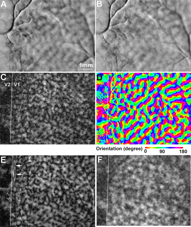
Spatial distributions of in information in areas V1 and V2. A-B: Averaged activation maps in response to horizontal and vertical gratings, respectively. The dark patches represent activated regions. C: The SVM-derived relative information map about stimulus orientation. The brightness of a pixel is proportional to the relative contribution of that pixel to the SVM classification. D: The orientation preference map in which the preferred orientation of each pixel is represented by pseudo-color. E: The orientation selectivity map. The brightness of a pixel is proportional to the selectivity of the pixel’s response for orientation. F: The accuracy map derived from the “search light” approach. The brightness of a pixel is proportional to the accuracy associated with the SVM classification that was applied to the 9x9 pixels centered at the given pixel.

To compare our results with those of previous imaging studies, we constructed an orientation preference map (Fig. 3D) and an orientation selectivity map (Fig. 3E) using the conventional method of vector summation (see METHODS). This conventional method analyzes the response amplitude at each pixel independently. The preference map represents the preferred stimulus orientation at each pixel, while the selectivity map represents the degree of modulation of the response amplitude by stimulus orientation. Fig. 3D shows the typical “pinwheel” organization of V1 columns that preferred various orientations (Bonhoeffer and Grinvald, 1991). Fig. 3E shows that the pixels at the pinwheel centers had lower selectivity for orientation than other pixels did. Note that the imaging signal integrates activity of many neurons, each of which might be highly selective for orientation, but in the pinwheel center each is tuned to a different orientation (Maldonado et al., 1997). The selectivity map also has a spatial pattern that is similar to the pattern of the relative information map (Fig. 3C). The correlation between these two maps were significant (r = 0.81, P < 10⁻¹⁰, t test on r). However, the artifacts associated with blood vessels are greatly suppressed in the relative information map, compared to the selectivity map (arrows in Fig. 3E). In addition, the SVM-derived information map takes into account the information encoded by the spatial patterns of responses across many pixels, whereas the selectivity map only measures the information encoded by the response amplitude at each pixel (see the next section). These results suggest that the spatial pattern of activity provides a better estimate of the relative distribution of information about a specific stimulus attributes than the response amplitude.

We obtained a relative information map about stimulus color from another animal in an experiment that used 9 uniformly colored stimuli (Fig. 4A). The image resolution here was 6.1 um/pixel, twice the resolution used in the orientation experiment that produced Fig. 3. To compare the distribution of information about color with that about orientation on an equal footing, we cropped a part of each single-trial image obtained from the orientation experiment, and enlarged it 2 folds. This new data set, after being filtered with the same DOG filter that was used in the color experiments, was then used to derive a new information map about orientation (Fig. 4B).

Figure 4.

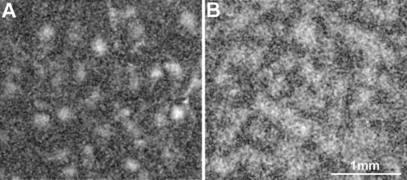
Comparison between the SVM-derived information maps about color (A) and orientation (B). Panel A was derived from an experiment that used uniform stimuli of 9 different colors, whereas panel B was from another experiment that used achromatic grating stimuli of 6 different orientations. These two maps show distinct spatial patterns.

Fig. 4 shows that the information about stimulus color was concentrated in small regions in striate cortex, while the information about orientation was more evenly distributed. This qualitative observation is supported by two quantitative analyses, which have been described previously in more details (Xiao et al., 2007b). First, the distributions of pixel intensity values in Figs. 3A and 3B were skewed differently. The distribution in Fig. 4A had a long right tail (skewness = 0.65), indicating the existence of a small number of pixels that carried much more color information than did most pixels. In contrast, the distribution in Fig. 4B had a long left-tail (skewness = −0.14), indicating the existence of a small number of pixels that carried much less orientation information than did most pixels. Second, the top 5% of pixels in Fig. 4A formed a small number of clusters, compared to those in Fig. 4B (205 vs. 371). This particular relationship held when different percentages of the most informative pixels were tested.

Information encoded by spatial patterns across different pixels

As a multivariate analysis, SVM analyzes the distribution of all samples in the high-dimensional space defined by each image pixel. Therefore, SVM is able to capture the information encoded by spatial patterns across different pixels among the samples. In contrast, a univariate analysis, such as the conventional t-map, analyzes each pixel independently, and is therefore unable to capture the pattern-based information. This difference between these two analyses is illustrated in the following simulation.

We generated 2 groups of artificial images of 8 pixels each. Each group has 100 images. A few examples of these images are shown in Fig. 5A. For each group, the value of each pixel was randomly chosen from a normal distribution that has a mean value of μ, except for the pixel at the first column and the second row, or P(1,2), which follows the distribution of the sum or difference of two normal functions. For each pixel in the first row, μ_group1 is slightly greater than μ _group2. More specifically, μ_group1 = 10⁴ and μ _group2 = 10⁴−4 for each pixel in the first row. Conversely, for each pixel in the second row, except for pixel (1,2), μ _group1 = 10⁴−4, μ _group2 = 10⁴. The standard deviation of these normal distributions is 30. To simulate a spatial pattern across a pair of pixels, we made P(1,2) in each image depend on P (1,1). For each image in group 1, P(1,2) = P(1,1) − d, where d is a random number from another normal distribution whose mean and standard deviation are 4 and 3, respectively. For each image in group 2, P(1,2) = P(1,1) + d (Fig. 5B). In other words, P(1,2) < P(1,1) for group 1, and P(1,2) > P(1,1) for group 2. Therefore, the spatial patterns are specific to the groups. As a comparison, we made the values of all other pixels independent of each other (e.g., Fig. 5C) so that there is no pattern across other pixels.

Figure 5.

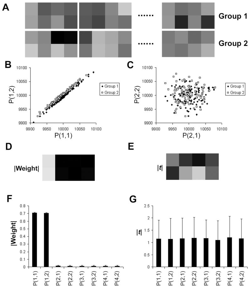
A simulation demonstrating the ability of the SVM-derived information map to reflect the information encoded by the spatial pattern of activity. A: Two groups of simulated images of 8 pixels each. Across group 1, a pixel in the first row has a slightly greater mean value than one in the second row. The opposite is true for group 2. B: The two pixels in the first column of each image are correlated, and the correlation is group specific. C: Pixels in the second column are independent of each other. This is also true for the third and forth column. D: Absolute values of different elements of the weight vector that is associated with the SVM classifier. The first column has the greatest value because only this column has group-specific patterns. E: Map of |t| that was calculated at each pixel independently. The values at the first column are comparable to those at other columns. F-G: Averaged |Weight| and |t| values across 200 iterations of simulation. It is clear that the |Weight| map, but not |t| map, reflects the distribution of information that is encoded in group-specific spatial patterns.

Due to our design, the two groups can be reliably discriminated based on the relationship between P(1,1) and P(1,2) in each image (Fig. 5B). Any discrimination based on other pixels is much less reliable, because of the lack of group-specific relationship among them. In other words, pixels (1,1) and (1,2) carry more information about the identity of each image than other pixels do. This distribution of information was successfully extracted by the SVM-derived relative information map when the SVM classification was applied to the artificial images (Fig. 5D). In contrast, this distribution of information was not reflected in the map of |t| (Fig. 5E), where t is the Student’s t value and was calculated at each pixel independently.

We ran 200 iterations of this simulation, and plotted the averaged relative information and |t| value for each pixel in Fig 4F and 4G, respectively. These two panels demonstrate that the SVM-derived relative information map, but not the |t| map, reflects the distribution of information that is encoded by the group-specific pattern across different pixels.

SVM for functional images

In a recent study on humans, SVM was used to classify two groups of fMRI images, each associated with a different brain state (Mourao-Miranda et al., 2005). The weight vector of the derived SVM classifier was interpreted as the activation map that best discriminates the two groups of images. When one group of images was associated with a specific stimulus, and the other group associated with no stimulus, the weight vector represented the single-condition activation map in response to the given stimulus.

We applied this technique to the images formed by intrinsic optical signals from the primate cortex in order to derive the single-condition map of V1 and V2 elicited by stimulation of either eye (Fig. 6A&B). Each panel is a scaled weight vector of the SVM classifier that discriminates the images acquired during the stimulation of the given eye from those acquired before the stimulation. The scale factor was calculated in the following way so that each panel also reflects the amplitude of the response to stimulation of the given eye. We first normalized the weight vector so that it had a length of 1. Second, we calculated the inner product between each image and the weight vector. Third, we averaged these inner products across each group. Finally, the scale factor was calculated by subtracting the average inner product associated with pre-stimulation from that associated with stimulation.

Figure 6.

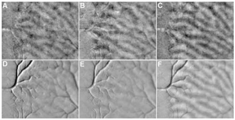
Ocular columns derived with SVM algorithm and subtraction. A-B: SVM-derived activation maps elicited by left and right eye stimulations, respectively. The images cortical region was the same as that shown in Fig. 3. C: Differential map between A and B. D-E: Subtraction-derived activation maps elicited by left and right eye stimulations, respectively. F: Differential map between D and E.

In Fig. 6A&B, the ocular dominance columns activated by either eye are clearly visible. As a comparison, we calculated conventional single-condition maps by subtracting the images taken before stimulation from those taken during stimulation (Fig. 6D&E). In these conventional single-condition maps, the ocular columns are obscured by significant artifacts associated with blood vessels. These results suggest that the SVM classification can successfully remove artifacts associated with blood vessels, because the spatial patterns of these artifacts are not specific to stimulus condition. SVM-derived single-condition maps thus have a high signal-to-noise (S/N) ratio compared to conventional maps. Fig. 6C&F show the SVM-derived and conventional differential maps, respectively, which were calculated by subtracting the single-condition ocular dominance maps of right eye from the maps of left eye. The ocular dominance columns are visible in the conventional differential maps because the artifacts that were not specific to stimulus conditions were removed by the subtraction.

Discussion

We have developed an SVM-based method to map the relative distribution of information that is encoded by the response pattern and amplitude. We have shown that the SVM-derived relative information map for orientation was significantly correlated with the orientation selectivity map derived from the conventional vector calculation (Fig. 3), suggesting that the former was a valid measurement of the information distribution. Compared with the selectivity map, the information map derived from our new method has two advantages. First, the information map attenuates the artifacts associated with blood vessels. Second, an SVM-derived information map reflects both the information encoded by the spatially distributed response pattern and that encoded by the response amplitude, as demonstrated in the simulated dataset (Fig. 5), whereas a selectivity map only reflects the information encoded by the response amplitude at each pixel. Because the variability in neuronal responses is correlated across a large area of cortex, the information encoded by the spatial pattern of responses is likely to be more reliable than that encoded by the response amplitude, and could therefore be the information used by animals for guiding their behavior (see Introduction).

Our new method is valid when the SVM classifier can successfully deduce the stimulus attribute from response images. For the data illustrated in Fig. 3, the accuracy of the deduction was 99.7%, significantly higher than the accuracy predicted by chance (16.7%, P < 10⁻¹⁰⁰, chi-square test). For another set of data where stimulus color was deduced from the response images (Fig. 4A), the accuracy was also significantly higher than chance (52.3% Vs. 11.1%, P < 10⁻¹⁰⁰). For these datasets, the information maps derived from the SVM classifiers are believed to represent the relative distribution of information across the imaged region. However, in cases where the accuracy of the SVM prediction is comparable to chance, the corresponding information map will not be reliable. In those cases, it is possible to improve the SVM accuracy by pre-processing the data with principle component analysis (PCA) to reduce the dimension of the vectors (Mourao-Miranda et al., 2005).

The SVM-derived information maps of orientation and color show distinct patterns in V1. The information about color is concentrated in small regions compared to the information about orientation. This result is consistent with the hypothesis that CO blobs and interblobs process color and orientation, respectively, because blobs are smaller than interblobs (Livingstone and Hubel, 1984). However, the orientation and color information maps described here were based on data that were acquired from different animals and were associated with different stimuli, which, in principle, might have contributed to the difference in spatial pattern of the color and orientation information maps. To address this concern, future studies need to use colored gratings as stimuli and derive the color and orientation information maps from the same set of data.

Although this paper describes the application of our new method to the images of intrinsic optical signals, the same method can also be applied to images acquired with other techniques, such as fMRI. Previous fMRI studies that mapped distribution of information have used the “search light” approach (Haynes et al., 2007). In this approach, SVM classification is applied to small regions at different locations, and the distribution of the SVM accuracy represents the distribution of information. We applied this approach to the data that produced Fig. 3, and obtained a map of accuracy using a square “search light” of 9 by 9 pixels (Fig. 3F). This map is also significantly correlated with the relative information map (r = 0.61, P < 10⁻⁴). But it lacks fine details about the information distribution compared to the map derived from our new method, because the “search light” functions like the kernel of a low-pass filter. The difference between these two maps becomes greater when the size of “search light” increases. Since the accuracy map can be used to assess the absolute amount of information at various locations of the “search light” (Haynes et al., 2007), which is not represented in our weight-based information map, it is desirable to compute both maps in order to determine the distribution of information in a given region.

We also showed that the weight vector of an SVM classifier can be used to map the response to a given stimulus, and the maps have a high S/N ratio compared to the conventional maps derived from subtraction (Fig. 6). The reason of this higher S/N ratio is that SVM, as a multivariate analysis, can detect the spatial patterns that are specific to stimulus condition.

Several previously proposed methods aiming at enhancing S/N ratio of activation maps are also based on multivariate analyses (Yokoo et al., 2001). These methods assume a normal distribution of noise, which may not be true in some cases. Since the SVM method does not require or assume any particular distribution of noise, it should have a wider application than the other multivariate analyses.

References

- Arieli A, Sterkin A, Grinvald A, Aertsen A. Dynamics of ongoing activity: explanation of the large variability in evoked cortical responses. Science. 1996;273:1868–1871. doi: 10.1126/science.273.5283.1868. [DOI] [PubMed] [Google Scholar]
- Bonhoeffer T, Grinvald A. Iso-orientation domains in cat visual cortex are arranged in pinwheel- like patterns. Nature. 1991;353:429–431. doi: 10.1038/353429a0. [DOI] [PubMed] [Google Scholar]
- Dean AF. The variability of discharge of simple cells in the cat striate cortex. Exp Brain Res. 1981;44:437–440. doi: 10.1007/BF00238837. [DOI] [PubMed] [Google Scholar]
- Gouras P. Trichromatic mechanisms in single cortical neurons. Science. 1970;168:489–492. doi: 10.1126/science.168.3930.489. [DOI] [PubMed] [Google Scholar]
- Gur M, Snodderly DM. High response reliability of neurons in primary visual cortex (V1) of alert, trained monkeys. Cereb Cortex. 2006;16:888–895. doi: 10.1093/cercor/bhj032. [DOI] [PubMed] [Google Scholar]
- Haynes JD, Sakai K, Rees G, Gilbert S, Frith C, Passingham RE. Reading hidden intentions in the human brain. Curr Biol. 2007;17:323–328. doi: 10.1016/j.cub.2006.11.072. [DOI] [PubMed] [Google Scholar]
- Hubel DH, Wiesel TN. Receptive fields and functional architecture of monkey striate cortex. Journal of Physiology. 1968;195:215–243. doi: 10.1113/jphysiol.1968.sp008455. [DOI] [PMC free article] [PubMed] [Google Scholar]
- Kara P, Reinagel P, Reid RC. Low response variability in simultaneously recorded retinal, thalamic, and cortical neurons. Neuron. 2000;27:635–646. doi: 10.1016/s0896-6273(00)00072-6. [DOI] [PubMed] [Google Scholar]
- Lennie P, Krauskopf J, Sclar G. Chromatic mechanisms in striate cortex of macaque. J Neurosci. 1990;10:649–669. doi: 10.1523/JNEUROSCI.10-02-00649.1990. [DOI] [PMC free article] [PubMed] [Google Scholar]
- Leventhal AG, Thompson KG, Liu D, Zhou Y, Ault SJ. Concomitant sensitivity to orientation, direction, and color of cells in layers 2, 3, and 4 of monkey striate cortex. Journal of Neuroscience. 1995;15:1808–1818. doi: 10.1523/JNEUROSCI.15-03-01808.1995. [DOI] [PMC free article] [PubMed] [Google Scholar]
- Livingstone MS, Hubel DH. Anatomy and physiology of a color system in the primate visual cortex. Journal of Neuroscience. 1984;4:309–356. doi: 10.1523/JNEUROSCI.04-01-00309.1984. [DOI] [PMC free article] [PubMed] [Google Scholar]
- Maldonado PE, Godecke I, Gray CM, Bonhoeffer T. Orientation selectivity in pinwheel centers in cat striate cortex. Science. 1997;276:1551–1555. doi: 10.1126/science.276.5318.1551. [DOI] [PubMed] [Google Scholar]
- Mourao-Miranda J, Bokde AL, Born C, Hampel H, Stetter M. Classifying brain states and determining the discriminating activation patterns: Support Vector Machine on functional MRI data. Neuroimage. 2005;28:980–995. doi: 10.1016/j.neuroimage.2005.06.070. [DOI] [PubMed] [Google Scholar]
- Schiller PH, Finlay BL, Volman SF. Short-term response variability of monkey striate neurons. Brain Res. 1976;105:347–349. doi: 10.1016/0006-8993(76)90432-7. [DOI] [PubMed] [Google Scholar]
- Snowden RJ, Treue S, Andersen RA. The response of neurons in areas V1 and MT of the alert rhesus monkey to moving random dot patterns. Exp Brain Res. 1992;88:389–400. doi: 10.1007/BF02259114. [DOI] [PubMed] [Google Scholar]
- Ts’o DY, Gilbert CD. The organization of chromatic and spatial interactions in the primate striate cortex. Journal of Neuroscience. 1988;8:1712–1727. doi: 10.1523/JNEUROSCI.08-05-01712.1988. [DOI] [PMC free article] [PubMed] [Google Scholar]
- Ts’o DY, Frostig RD, Lieke EE, Grinvald A. Functional organization of primate visual cortex revealed by high resolution optical imaging. Science. 1990;249:417–420. doi: 10.1126/science.2165630. [DOI] [PubMed] [Google Scholar]
- Vapnik V. Statistical Learning Theory. New York, NY: John Wiley & Sons, Inc; 1998. [Google Scholar]
- Wang Y, Xiao Y, Felleman DJ. V2 thin stripes contain spatially organized representations of achromatic luminance change. Cereb Cortex. 2007;17:116–129. doi: 10.1093/cercor/bhj131. [DOI] [PubMed] [Google Scholar]
- Xiao Y, Wang Y, Felleman DJ. A spatially organized representation of colour in macaque cortical area V2. Nature. 2003;421:535–539. doi: 10.1038/nature01372. [DOI] [PubMed] [Google Scholar]
- Xiao Y, Casti A, Xiao J, Kaplan E. Hue maps in primate striate cortex. Neuroimage. 2007a;35:771–786. doi: 10.1016/j.neuroimage.2006.11.059. [DOI] [PMC free article] [PubMed] [Google Scholar]
- Xiao Y, Rao R, Cecchi G, Kaplan E. Cortical representation of information about visual attributes: one network or many?. Proceedings of the International Joint Conference on Neural Networks, IJCNN’07; Orlando, USA. New York: IEEE; 2007b. [Google Scholar]
- Yokoo T, Knight BW, Sirovich L. An optimization approach to signal extraction from noisy multivariate data. Neuroimage. 2001;14:1309–1326. doi: 10.1006/nimg.2001.0950. [DOI] [PubMed] [Google Scholar]
- Yoshioka T, Dow BM. Color, orientation and cytochrome oxidase reactivity in areas V1, V2 and V4 of macaque monkey visual cortex. Behavioural Brain Research. 1996;76:71–88. doi: 10.1016/0166-4328(95)00184-0. [DOI] [PubMed] [Google Scholar]