Modeling response signal and response time data

Abstract

The diffusion model (Ratcliff, 1978) and the leaky competing accumulator model (LCA, Usher & McClelland, 2001) were tested against two-choice data collected from the same subjects with the standard response time procedure and the response signal procedure. In the response signal procedure, a stimulus is presented and then, at one of a number of experimenter-determined times, a signal to respond is presented. The models were fit to the data from the two procedures simultaneously under the assumption that responses in the response signal procedure were based on a mixture of decision processes that had already terminated at response boundaries before the signal and decision processes that had not yet terminated. In the latter case, decisions were based on partial information in one variant of each model or on guessing in a second variant. Both variants of the diffusion model fit the data well and both fit better than either variant of the LCA model, although the differences in numerical goodness-of-fit measures were not large enough to allow decisive selection between the models.

1. Introduction

Since the 1970s, the response signal paradigm has been attractive to cognitive psychologists because it tracks, in a manner that appears to be quite direct, the time course with which information becomes available to decision processes. Other paradigms, such as those using standard response time (RT) measures, only allow information growth as a function of time to be determined indirectly, for example, through models of processing. In this article, I explore how current models for two-choice decisions can explain response signal data.

In a response signal experiment, a test item is presented and then it is followed at some time lag by a signal that tells the subject to respond. Several different time lags are used, in random order across trials, varying from such a short amount of time between test item and signal that performance is at chance to an amount of time at which performance asymptotes. Subjects are asked to respond within 200–300 ms of the signal, and the dependent variable is accuracy. Because the method provides snapshots of accuracy across the lags, it yields a map of the growth of accuracy as a function of time. Usually, the measure of accuracy is d′, with one experimental condition taken as baseline and the other conditions scaled against it. The response signal paradigm has been used to examine a number of experimental questions in two-choice tasks in experimental psychology and Reed (1976) argued that it is superior to deadline procedures, which fix the lag between stimulus and signal at a constant within blocks of trials, because subjects are informed of the deadline ahead of time and can alter their retrieval strategy as a function of the deadline (see also Corbett & Wickelgren, 1978; Dosher, 1976, 1979, 1981, 1982, 1984; McElree & Dosher, 1993; Ratcliff, 1980, 1981; Reed, 1973, 1976; Schouten & Bekker, 1967; Wickelgren, 1977; Wickelgren and Corbett, 1977).

The response signal procedure has been used to measure three characteristics of processing: the point in time at which the amount of information available to the decision process is sufficient for accuracy to begin to grow above chance, the rate at which the amount of information grows toward asymptotic accuracy, and the level of asymptotic accuracy. In contrast, the standard RT procedure provides an estimate of the time to make a decision but, in the absence of a theory of processing, it cannot be used to determine the time at which information begins to be available, the rate of growth, or the level of asymptotic accuracy. It has also been argued that the standard RT procedure provides an estimate of only a single point on the function that maps the growth of accuracy over time (e.g. Dosher, 1984). In the experiment presented below, I collected both response signal and standard RT data from the same subjects in order to examine whether and how models can simultaneously explain the growth of accuracy over time in the response signal paradigm and all the data from the standard RT paradigm (accuracy and RT distributions for both correct and error responses). The main question was how the constraints of accounting for both kinds of data jointly might impact theoretical interpretations of how information becomes available to decision processes over time.

Often in previous research, the analysis of response signal data is not theory-based (e.g. Corbett & Wickelgren, 1978; Dosher, 1976, 1979, 1981, 1982, 1984; Hintzman & Curran, 1997; McElree & Dosher, 1993; Ratcliff, 1980, 1981; Reed, 1973, 1976; Schouten & Bekker, 1967; Wickelgren, 1977; Wickelgren, Corbett, & Dosher, 1980, 1977). Usually, an exponential function for growth to asymptote over time is fit to the d′ values for the response signal lags:

$$d^{\prime }(t)=d_{\text{a}}^{\prime }(1-exp(-(t-T_0)/\tau )),\text{for }{T}_0>0,$$ (1)

Where $d_{\text{a}}^{\prime }$ is the asymptotic level of accuracy, T₀ is the time intercept at which accuracy begins to grow above chance, and τ is the time constant for exponential rate of growth to asymptote. Differences among the values of intercept, rate, and asymptote across experimental conditions are then used to assess the effects of various independent variables on the time course of information accumulation and also to evaluate predictions about how these features of performance should behave (Corbett & Wickelgren, 1978; Dosher, 1976, 1979, 1981, 1982, 1984; McElree & Dosher, 1993; Ratcliff, 1981; Reed, 1973, 1976). The exponential function generally provides good fits to response signal data. McElree and Dosher (1989) compared the exponential to the expression for growth of accuracy derived from the diffusion model proposed by Ratcliff (1978), and found that the exponential was slightly superior to the diffusion model expression, but the differences were small. Wagenmakers, Ratcliff, Gomez, and Iverson (2004) used Monte Carlo simulations of the two expressions to compute how many observations would be needed to discriminate them, and found that, for typical data, about 2000 observations per experimental condition would be needed to discriminate them at a .95 probability level.

The major problem with the exponential function as a summary of the d′ growth function is that it is not theoretically based. There is no model of underlying cognitive processes that gives rise to the exponential function and no obvious theoretical way to relate the exponential function from response signal data to data from the standard RT task.

The two-choice models explored in this article are sequential sampling models, the diffusion model (Ratcliff, 1978, 1981, 1985, 1988, 2002; Ratcliff & Rouder, 1998, 2000; Ratcliff & Smith, 2004; Ratcliff & Tuerlinckx, 2002; Ratcliff, Gomez, & McKoon, 2004; Ratcliff, Van Zandt, & McKoon, 1999) and the leaky competing accumulator model (the LCA model, Usher & McClelland, 2001). These two models were chosen because they have been applied to response signal data previously and because Usher and McClelland argued that the two models can be discriminated with response signal data. Both models assume that noisy information is accumulated over time from a starting point toward one of two decision criteria, or boundaries. In a standard RT experiment, a response is initiated when the amount of accumulated information reaches one or the other of the boundaries. In a response signal experiment, on many trials, a response is required before the accumulated information reaches a boundary. To handle this, Ratcliff (1978) assumed that the decision process proceeds without boundaries, and a decision is based on the position of the process at the time of the response signal, that is, whether the amount of accumulated information is above or below the starting point. Later, Ratcliff (1988) proposed that the decision boundaries are retained and that responses are based on a mixture of processes, those that have already hit a boundary at the time of the response signal and those that have not; in the latter case, a decision is based on the position of the process. Usher and McClelland (2001) made the same assumption as Ratcliff (1978), that decisions in the response signal paradigm are based on the position of the process at the time of the response signal, with decision criteria removed.

In this article, I jointly fit data for the same subjects from the response signal paradigm and the standard RT paradigm for both the diffusion model and the LCA model. The task used for both paradigms was a signal detection task: arrays of between 13 and 87 dots were presented to subjects and they were asked to decide for each array whether the number of dots was large or small. The goal was that the models account for all aspects of both kinds of data with as many parameters as possible kept the same across the two tasks.

2. The diffusion model

The diffusion model was developed to explain the processes by which two-choice decisions are made. The model applies only to relatively fast two-choice decisions (mean RTs less than about 1000–1500 ms) and only to decisions that are a single-stage decision process (as opposed to the multiple-stage processes that might be involved in, for example, reasoning tasks or card sorting tasks). The model has been successful in explaining the data in a number of areas including perceptual tasks (Ratcliff, 2002; Ratcliff & Rouder, 1998, 2000; Ratcliff, Thapar, & McKoon, 2003; Thapar, Ratcliff, & McKoon, 2003), perception and attention tasks (Smith, Ratcliff, & Wolfgang, 2004), signal detection tasks (Ratcliff, Thapar, & McKoon, 2001; Ratcliff et al., 1999), lexical decision (Ratcliff, Gomez, & McKoon, 2004; Ratcliff, Thapar, Gomez, & McKoon, 2004), recognition memory (Ratcliff, 1978; Ratcliff, Thapar, & McKoon, 2004), and perceptual matching (Ratcliff, 1981). Other diffusion models have been applied in decision making (Busemeyer & Townsend, 1993; Roe, Busemeyer, & Townsend, 2001) and simple RT (Smith, 1995) tasks.

The heart of the diffusion model is depicted in the middle panel of Fig. 1. Information from a stimulus is accumulated continuously over time from a starting point z to decision criteria (response boundaries) at 0 and a, one criterion for each of the two responses. The boundaries are labeled “large” and “small,” the two response choices for the experiment presented below. The information from a stimulus is noisy and the growth of accumulated evidence is highly variable over the course of a decision process, as shown by the variable paths in the panel. The mean rate of information accumulation is called drift rate, ξ. Its variability is assumed to come from a normal distribution with standard deviation s, where s₂ is called the diffusion coefficient. s is a scaling parameter of the model; in other words, if the parameter were doubled, other parameters of the model could be doubled to produce exactly the same predictions. In the fits presented here, s is set to a fixed value, 0.1, that matches other applications of the model (e.g. Ratcliff, 1978, 1988, 2002; Ratcliff & Rouder, 1998, 2000; Ratcliff, Thapar, & McKoon, 2001, 2003, 2004; Ratcliff & Van Zandt, 1999).

Fig. 1.

An illustration of the diffusion and LCA models. The top panel illustrates the nondecision component of RT and the decision components of the diffusion model. The middle panel illustrates the diffusion decision process and the bottom panel illustrates the LCA model accumulators.

Because of the variability in the path of evidence accumulation, decision processes with the same drift rate hit the boundaries at different times, producing RT distributions, and a decision process with drift toward one of the boundaries can hit the wrong boundary by mistake, producing an error. If the response boundaries are moved further away from the starting point, the probability of a process with drift toward the correct boundary hitting the other boundary in error is reduced, thus increasing accuracy (and RT). The drift rate for stimuli in difficult conditions of an experiment is smaller than the drift rate for stimuli in easier conditions, which results in longer RTs and lower accuracy for difficult compared with easy conditions. RT distributions are right skewed because of the geometry of the decision process. If drift rate decreases, RTs increase, with a relatively small change in the leading edge of the RT distribution and a larger change in the tail of the distribution.

Not shown in Fig. 1 is the drift criterion, which serves the same function as the criterion in signal detection theory: it separates stimuli into those with positive drift rates and those with negative drift rates, like the signal detection criterion separates stimuli into signal and noise. Also like the criterion in signal detection theory, the value of the drift criterion can vary with experimental manipulations such as differential payoffs for the two responses or the relative proportions of test items for which the two responses are correct (Ashby, 1983; Link, 1975; Link & Heath, 1975; Ratcliff, 1978, 1985, 2002; Ratcliff et al., 1999). Changing the drift criterion from one block of trials to another with manipulations like these is equivalent to adding or subtracting a constant to the drift rates for all stimuli in one block compared to another (Ratcliff, 2002), again just as in signal detection theory. Usually the drift criterion is set to zero and the drift rates set relative to this zero point, although for some manipulations, the criterion might change across blocks of trials (e.g. Ratcliff & Smith, 2004; see also Ratcliff, 1985; Ratcliff et al., 1999). Here we set the drift criterion to zero for the regular RT task and allow it to differ for the response signal task and therefore account for differential bias between them.

Variability in processing across trials is implemented in several components of the diffusion model. First, the starting point varies across trials with a rectangular distribution with mean z and range s_z (Laming, 1968; Ratcliff et al., 1999). Second, the drift rate for nominally equivalent stimuli, that is, stimuli that are in the same experimental condition, varies across trials and is assumed to be normally distributed with mean v and standard deviation η (Ratcliff, 1978; Ratcliff et al., 1999).

With variability in drift rate and variability in starting point across trials, Ratcliff and Rouder (1998) and Ratcliff et al. (1999; see also Ratcliff, 1981; Smith & Vickers, 1988; Van Zandt & Ratcliff, 1995) showed that the diffusion model accounts for all of the patterns of relative speeds of correct and error responses that have been observed empirically. Error responses are sometimes faster than correct responses (this usually occurs when RTs are short or the experiment is easy), sometimes they are slower (usually when RTs are long or the experiment is difficult), and sometimes there is a crossover pattern within an experiment, such that errors are faster than correct responses in easy conditions and slower in difficult conditions (Ratcliff & Rouder, 2000; Ratcliff et al., 1999; Smith & Vickers, 1988). With speed–accuracy manipulations, errors are often slower than correct responses when subjects are asked to make their responses as accurate as possible but faster than correct responses when subjects are asked to make their responses as fast as possible (Ratcliff & Smith, 2004). The diffusion model can explain all of these patterns but, assuming that the only parameter of the model that can vary with stimulus difficulty is drift rate, the model cannot account for a pattern that has never been obtain empirically (to my knowledge): errors slower than correct responses in easy conditions and faster in difficult conditions.

Besides the decision process, shown in the middle panel of Fig. 1, there are nondecision components of processing such as stimulus encoding and response execution. These are combined in the model into a single value that is assumed to be variable across trials with a rectangular distribution (for simplicity) with mean T_er and range s_t. The top panel of Fig. 1 shows the total RT for a test item as the sum of the time for the nondecision components and decision time. In practice, the standard deviation of the distribution of decision times is much larger than the standard deviation of the distribution of nondecision times, so the shape of the RT distribution is determined almost completely by the shape of the distribution of decision times; and the shape of the nondecision distribution has almost no effect on predicted RT distribution shape (Ratcliff & Tuerlinckx, 2002, Fig. 11). Variability in the nondecision component of RT has two effects on model predictions: the leading edge of the RT distribution has greater variability across experimental conditions than would otherwise be the case, and the rise in the leading edge of the RT distribution is more gradual than it would otherwise be. This latter effect was crucial to a diffusion model account of lexical decision data (Ratcliff et al., 2004).

Expressions for the distributions of RTs and accuracy values for the diffusion model, adapted from Feller (1968), are provided in Ratcliff (1978) and Ratcliff et al. (1999). In fitting the model to data, these expressions are used to generate predicted RTs and accuracy values.

3. The leaky competing accumulator model

The LCA model (Usher & McClelland, 2001) was developed as an alternative to the diffusion model with the aim of implementing neurobiological principles that the authors felt should be incorporated into RT models, especially mutual inhibition mechanisms and decay of information across time.

In the LCA model (Usher & McClelland, 2001), like the diffusion model, information is accumulated continuously over time. There are two accumulators, one for each response, as shown in the bottom panel of Fig. 1, and a response is made when the amount of information in one of the counters reaches its criterion amount. The rate of accumulation, the equivalent of drift rate in the diffusion model, is a combination of three components. The first is the input from the stimulus (v), with a different value for each experimental condition. If the input to one of the accumulators is v, the input to the other is 1 − v so that the sum of the two rates is 1. The second component is decay in the amount of accumulated information, k, with decay growing as the amount of information in the accumulator grows, and the third is inhibition from the other accumulator, β, with the amount of inhibition growing as the amount of information in the other accumulator grows. If the amount of inhibition is large, the model exhibits features similar to the diffusion model because an increase in accumulated information for one of the response choices produces a decrease for the other choice. The assumption of cross-coupling between accumulators makes the model similar to an earlier, discrete-time model proposed by Heuer (1987).

Just as in the diffusion model, information accumulation is assumed to be variable. The distribution is assumed to be normal with standard deviation σ. Because of this variability, accumulated information can reach the wrong criterion, resulting in an error. Because of the decay and inhibition in the accumulation rates, the tails of RT distributions are longer than would be produced without these factors (cf., Vickers, 1970, 1979; Vickers, Caudrey, & Willson, 1971), which leads to good matches with the skewed shape of empirical distributions.

The expression for the change in the amount of accumulated information at time t in counter i, is

$$\text{d}{x}_i=\left[{\upsilon }_i-k{x}_i-\beta \sum _{j\ne i}{x}_j\right]\frac{\text{d}t}{\tau }+\sigma \sqrt{\frac{\text{d}t}{\tau }},$$ (2)

where dt/τ is set to .1 corresponding to 10 ms steps as in Usher and McClelland (2001). The amount of accumulated information is not allowed to take on values below zero, so if it is computed to be below zero, it is reset to zero; this constraint is written as x_i → max(x_i, 0) and it introduces nonlinearity into the model.

Just as for the drift criterion in the diffusion model, the LCA model has an accumulation rate criterion to accommodate a difference in bias between the response signal task and the RT task. The unbiased accumulation rate for each accumulator is .5, which means they would be accumulating information at the same rate.

The LCA model without across trial variability for any of its components predicts errors slower than correct responses. To produce errors faster than correct responses and the crossover pattern such that errors are faster than correct responses for easy conditions and slower for difficult conditions, Usher and McClelland assumed variability in the accumulators’ starting points, just as is assumed in random walk (Laming, 1968) and diffusion models.

In the diffusion model, moving a boundary position is equivalent to moving the starting point. Moving the starting point an amount y toward one boundary is the same as moving that boundary an amount y toward the starting point and the other boundary an amount y away from the starting point. In the LCA model, changing the starting point is not equivalent to changing a boundary position because decay is a function of the distance of the accumulated amount of evidence from the starting point. Increasing the starting point by an amount y increases decay by an amount proportional to y, but with fixed starting point, reducing the boundary by y has no effect on decay. Usher and McClelland (2001) implemented variability in starting point by assuming rectangular distributions of the starting points with minimums at zero. I implemented this version of the model and also another version with variable starting points that were offset from zero by unequal amounts. This latter version had two additional parameters (one offset amount for each accumulator). I examined this version of the model to explore whether its increased flexibility might lead to better fits to data.

Like the diffusion model, nondecision components of processing are combined into one parameter. To provide the model with flexibility equivalent to the diffusion model, the nondecision components of processing were assumed to vary in the same way as for the diffusion model, a rectangular distribution with range s_t and mean T_er (Ratcliff & Smith, 2004).

No explicit solution is known for Eq. (2) in conjunction with the nonlinearity that constrains the amount of accumulated evidence to be positive. Thus, as in Usher and McClelland (2001), predictions from the model were obtained by simulation. In the fits of the model to the data described here, 20,000 simulations of the decision process per experimental condition were used to compute the probabilities of the two responses for the response signal task and the standard RT task and the RT distributions for the two responses for the RT task.

4. Modeling the response signal paradigm

For the standard RT paradigm, responses are made when the amount of accumulated information reaches a response boundary. For the response signal paradigm, responses must often be made before a boundary is reached. To model this situation, researchers in the past have made the simple assumption that the response boundaries are removed from the decision process and so no decision process can ever reach a boundary. When the signal to respond is given, subjects make their decision according to the amount of accumulated information; for the diffusion model (Ratcliff, 1978), whether the amount is above or below the starting point, and for the LCA model (Usher & McClelland, 2001), which accumulator has the most accumulated information.

For the diffusion model (Ratcliff, 1978), when there are no boundaries, the expression for position in the process (the amount of accumulated information) as a function of time is

$$h(x,t)=\frac{1}{\sqrt{2\pi t{s}^2}}exp\left[-\frac{{(x-\xi t)}^2}{2t{s}^2}\right].$$ (3)

Integrating over the normal distribution of drift rates across trials with standard deviation η, the expression for position is

$$y(x,t)=\frac{1}{\sqrt{2\pi t({\eta }^{2}t+s^2)}}exp\left[-\frac{{(x-\upsilon t)}^2}{2t({\eta }^{2}t+s^2)}\right].$$ (4)

Because this distribution is normal with mean vt and standard deviation $\sqrt{t({\eta }^{2}t+s^2)}$, and d′ is defined as the difference in means divided by the standard deviation, the growth of d′ as a function of time for two conditions with drift rates v₁ and v₂ is

$$d^{\prime }(t)=\frac{d_{\text{asy}}^{\prime }}{\sqrt{1+\frac{s^2}{{\eta }^{2}t}}},$$ (5)

where $d_{\text{asy}}^{\prime }=({\upsilon }_1-{\upsilon }_2)/\eta$ (see Ratcliff, 1978, 1980). As mentioned earlier, this expression leads to fits of the diffusion model to data that are minimally different from fits using the exponential function.

Recently, Usher and McClelland (2001) compared the diffusion model and the Ornstein–Uhlenbeck (OU) model using data from a response signal experiment. The OU model is a good approximation of the LCA model, and they used it to fit response signal data because analytic solutions are available. For both the diffusion and OU models, the assumption was that response boundaries were removed. The OU model provided a somewhat better fit to the data than the diffusion model. However, the models that were considered are the simplest versions and it is likely that with more realistic processing assumptions, such as an assumption of variability in the nondecision components of processing (T_er), the difference between the models would have been significantly reduced (this assumption would reduce the steepness of the initial rise, the place where the two models differed).

In this article, it is argued that implementing response signal decision processes without decision boundaries is an oversimplification. For long signal durations (e.g., 2000 or 1500 ms), it is clear that subjects have already decided which response they are going to make and are simply waiting for the signal. This suggests a different implementation: The accumulation of information proceeds in the standard way, the same way as for standard RT paradigms, with two response boundaries. When a signal is presented, the decision process can be in one of two states: either the process has already reached a boundary or it has not. If the process has already reached a boundary, the response corresponding to that boundary is produced. If not, then one of two assumptions can be made: either partial information from the decision process can be used to make the decision, or that it cannot be used, in which case the response is a guess.

For the diffusion model, the two possible states at the time of a response signal are illustrated in Fig. 2 with processes for which the mean drift rate v is large and positive. In the top panel, at time T₁, some processes have already reached a boundary (those corresponding to the portions of the RT distributions immediately to the left of T₁) and some have not (those corresponding to the portions of the RT distributions immediately to the right of T₁). If partial information is available to be used in making a decision (middle panel of Fig. 2), then if the process is above the midpoint (a/2), one decision is made, and if it is below the midpoint, the other decision is made. The total probability of a “large” response at time T₁ is the sum of the black areas in the middle panel. To give a second illustration, at a later time, T₂, the probability of a “small” response is the sum of the grey areas. Accuracy grows from time T₁ to T₂ because more processes terminate and these are more accurate than decisions based on nonterminated processes. The accuracy of nonterminated processes increases only by a small amount as a function of time, and only across shorter response signal lags (see Ratcliff, 1988). If partial information is not available to the decision process, then for processes that have not terminated, a guess is produced with some fixed probability (Fig. 2, bottom panel) and accuracy grows as processes terminate at the boundaries. The two assumptions about availability of partial information provide two versions of the diffusion model.

Fig. 2.

An illustration of terminated and nonterminated processes. The top panel shows the distributions for “large” and “small” responses for terminated and nonterminated processes at times T₁ and T₂. The middle panel shows the probability of a “large” response at T₁, if decision processes have access to partial information; it is the combination of the two black densities. The probability of a “small” response at T₂ is the combination of the two grey densities. The bottom panel shows the probabilities of “large” and “small” responses if partial information is not available and nonterminated processes lead to guesses.

The criterion for deciding between the response alternatives on the basis of partial information is set at the midpoint between 0 and a (i.e., a/2) so that responses at the very earliest response signal lags can be biased according to where the starting point z is located relative to a/2. For example, if z is between a/2 and the “large” criterion, then at very short response signal lags, the position of decision processes will tend to be closer to the “large” criterion than the “small” criterion. As will be seen in the data, some subjects show this kind of bias.

For the LCA model, there are the same two possible states at the time of a response signal; either a decision process has terminated or it has not. If it has, the appropriate response is produced. If not, and partial information is not available, then a guess is produced with some fixed probability. If partial information is available, then the response appropriate for whichever accumulator has the most accumulated information is produced.

The experiment in this article allows both the partial information and guessing versions of the diffusion and LCA models to be tested. These versions were also compared with versions of the models that assume no response boundaries.

5. Availability of partial information

The issue of whether partial information can be used by decision processes when subjects are asked to respond at a signal was examined in a set of papers in the late 1980s by Meyer and colleagues (Kounios, Osman, & Meyer, 1987; Meyer, Irwin, Osman, & Kounios, 1988; see also Meyer, Yantis, Osman, & Smith, 1985; Ratcliff, 1988). They used a paradigm in which on any given trial, either subjects were asked to respond before or at a signal, or there was no signal and they completed a normal response; these two kinds of trials were randomly intermixed. Responses for signal trials were assumed to represent a mixture, some responses based on already terminated processes and the others based on partial information. For each response signal lag, for the responses based on already terminated processes, Meyer and colleagues assumed that their accuracy was the same as the accuracy of responses on nonsignal trials for which the response was made at or before the time of the signal. They subtracted this accuracy value from the total accuracy for responses at that lag to obtain the accuracy of responses based on partial information. They found that in some tasks, responses based on this measure of partial information were above chance, but in other tasks, they were at chance.

With the assumption that decisions in the diffusion model could be based on partial information, Ratcliff (1988) showed that the diffusion model could account quantitatively for Meyer and colleagues’ data. Ratcliff (1988) also proposed that results from the standard response signal procedure could be explained in the same way, as a probability mixture of terminated processes and nonterminated processes, but no attempt was made to fit response signal data quantitatively.

De Jong (1991) proposed an alternative account of the results from Meyer et al.’s paradigm. He assumed that all responses based on partial information were at chance (i.e., guesses) and that the apparent above chance accuracy was due to a speed up of regular processes when a response signal was presented. De Jong’s simulations showed that this assumption was sufficient to account for the greater than chance estimates of guessing accuracy obtained in two of Meyer et al.’s experiments.

In this article, the guessing versions of the diffusion and LCA models use an assumption like De Jong’s (but without the assumption of a speed-up in processing) as an alternative to the versions of the models that allow access to partial information. To foreshadow the results, I find that the guessing and partial information models cannot be discriminated on the basis of response signal and RT data.

5.1. Predictions for partial information as a function of time

For the diffusion model, the distribution of the positions x of decision processes at time t is given by

$$p(x,t)=exp\left[\frac{\xi (x-z)}{s^2}\right]\sum _{n=1}^{\infty }\frac{2}{a}sin\left(\frac{n\pi z}{a}\right)sin\left(\frac{n\pi x}{a}\right)exp\left[-\frac{1}{2}\left(\frac{{\xi }^2}{s^2}+\frac{n^2{\pi }^2{s}^2}{a^2}\right)t\right],$$ (6)

where s² is the diffusion coefficient, z is the starting point, a is the separation between the boundaries, and ξ is the drift rate. For model fitting, the expression in Eq. (6) must be integrated over the normal distribution of drift rates and the uniform distribution of starting points to include variability in drift rate and starting point across trials. This was accomplished with numerical integration using Gaussian quadrature. The series in Eq. (6) must be summed until it converges; this means that terms have to be added until subsequent terms become so small that they do not affect the total (i.e., the series has converged to within some criterion, e.g., 10^{− 5}). Then, to obtain the probability of choosing each response alternative, the proportion of processes between 0 and a/2 (for the negative alternative) and between a/2 and a (for the positive alternative) is calculated by integrating the expression for the density over position.

For the LCA model, the distributions of positions of processes in the two accumulators were simulated, with variability in parameters across trials implemented by selecting random deviates from the distributions of the parameters. Partial information was modeled by assuming that when the signal to respond was presented, if the process had not terminated, the process that had the greater amount of information was chosen.

6. Experiment

The aim was to use the diffusion model and the LCA model (in their partial information versions and their guessing versions) to simultaneously account for data from the standard RT task and response signal data. For the standard task, accuracy, correct and error RTs, and their distributions for each experimental condition were the targets for modeling. For the response signal data, the probabilities of each response alternative for each condition were the targets for modeling. In most previous response signal studies, d′ values have been the target data, where d′ is computed by choosing accuracy for one experimental condition as baseline and scaling accuracy for the other experimental conditions against it. In almost all such studies, the two sets of probabilities that enter the d′ computation have not been modeled separately. I model them separately here to ensure that the models can deal with biases toward one or the other response alternative as well as d′ discriminability.

The task chosen to provide the data against which the models would be tested had to meet several requirements. First, it had to be a task that the models had successfully fit (e.g., Experiment 1, Ratcliff & Smith, 2004). Second, in order to stringently test the models, it had to be a task for which difficulty could be manipulated such that accuracy could vary from floor (near chance) to ceiling (near 100% correct) and for which speed–accuracy criteria could be manipulated. The paradigm chosen was a variant of signal detection that is used extensively in probability matching and categorization (Ashby & Gott, 1988; Espinoza-Varas &Watson, 1994; Lee & Janke, 1964; Nosofsky, 1987; Ratcliff & Rouder, 1998; Ratcliff, Thapar, & McKoon, 2001; Ratcliff & Van Zandt, 1999; Vickers, 1979). An array of dots is presented on a computer screen and a subject is asked to decide whether the number of dots is “large” or “small” (Fig. 3). In other experiments, arrays of asterisks have been used, but I chose to use dots here to make the signal to respond, a row of capital R’s, more distinctive.

Fig. 3.

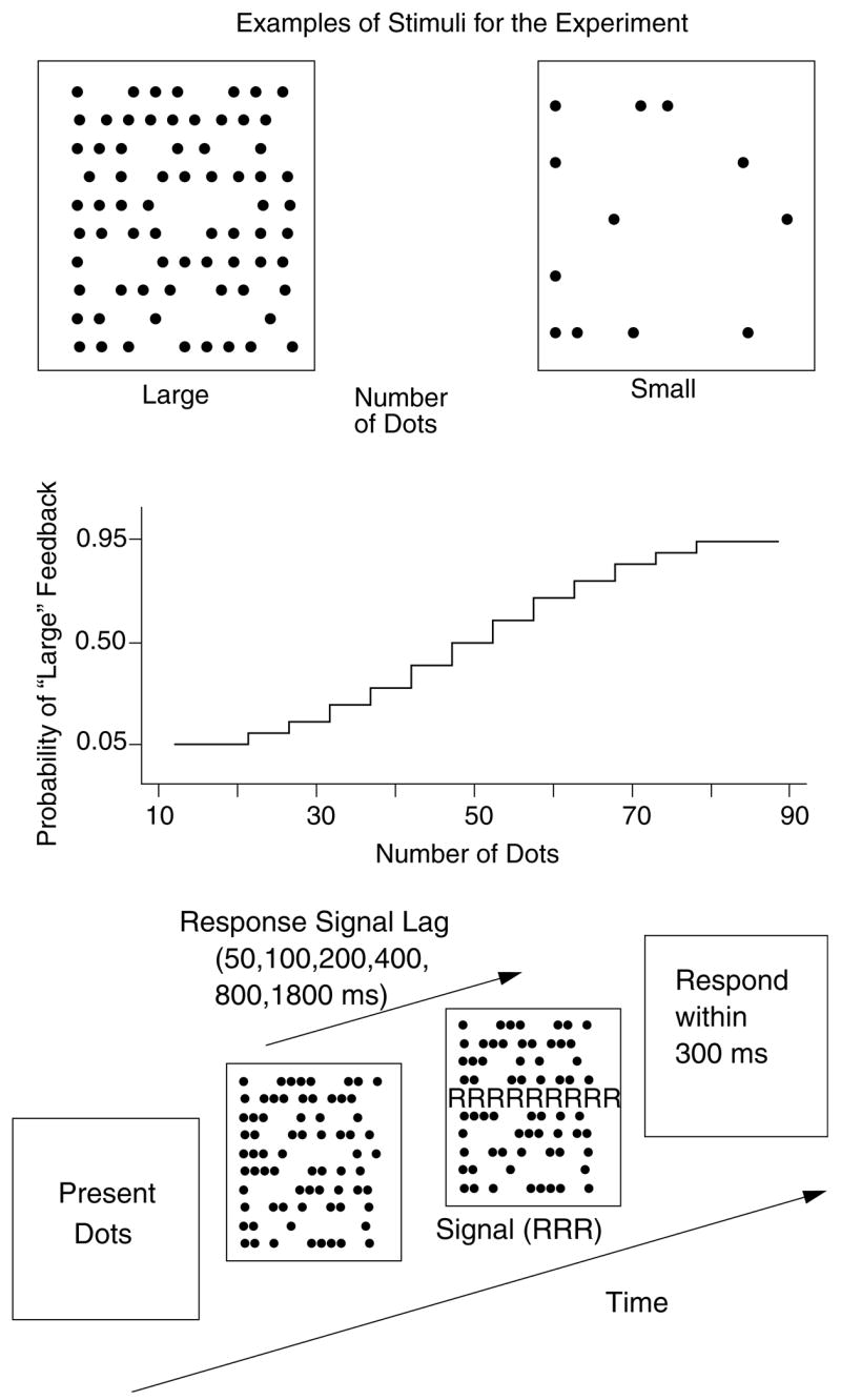
A illustration of the experimental paradigm. The top panel shows two sample stimulus dot arrays, the middle panel shows feedback probabilities, and the bottom panel shows the sequence of events in a response signal trial.

In each block of 75 trials, stimuli containing all possible numbers of dots between 13 and 87 dots were presented in random order with the dots presented in random positions in a 10 by 10 array. Feedback as to which response was correct was provided after each trial and it was variable according to the function shown in Fig. 3. For example, 13–22 dots received “small” feedback 95% of the time, 78–87 dots received “large” feedback 95% of the time, 43–47 dots received “small” feedback 40% of the time, and so on.

This type of signal detection paradigm allows the probabilities of the two responses, “large” and “small,” to be varied in small steps from a high probability of one of the responses being given feedback as correct to a high probability of the other response being given feedback as correct, with the most difficult conditions being in the middle range of the number of dots because the feedback is about as likely to indicate that a “small” response is correct as to indicate that a “large” response is correct. Varying difficulty over this large range of values forces a model to account for the relationships between response probabilities and response speeds at all levels of response probability. It is likely that the range of difficulty is in large part due to uncertainty about the number of dots rather than the variable nature of the feedback because in a recent experiment, providing accurate feedback had a relatively small effect on the patterns of data.

6.1. Method

6.1.1. Subjects

Seven undergraduate students were recruited from the Northwestern undergraduate population by flyers posted around campus and each was paid $8 per session, 14 sessions for three subjects and 18 sessions for four subjects.

6.1.2. Stimuli

The dots were displayed in a 10 × 10 grid in the upper left corner of a VGA monitor, subtending a visual angle of 4.30° horizontally and 7.20° vertically. They were clearly visible, light characters presented against a dark background. The response signal was a row of R’s that replaced the sixth row of dots. The VGA monitors were driven by IBM 486-style microcomputers that controlled stimulus presentation time and recorded responses and RTs.

6.1.3. Design and procedure

Stimuli were presented in blocks of 75 trials, with a subject-timed rest between each block. Stimuli consisted of all possible numbers of dots between 13 and 87 inclusive, displayed in random positions in the array. Subjects were instructed that the number of dots on each trial was selected at random from one of two groups of numbers, a “small” group and a “large” group, and that the small group had fewer dots on average than the large group. A subject’s task was to decide whether the number of dots presented came from the small group, in which case they were to press the “Z” key on the computer keyboard, or the large group, in which case they were to press the “?” key. The subjects understood that they could not be completely accurate, that numbers from the middle of the range (e.g., 50) could have come from either distribution, and that their task was to give their best judgment. Subjects were fully informed about this ambiguity, using X-ray diagnosis as an illustration of the ambiguity in signal detection tasks of this kind.

Feedback was selected from a discrete array. For each range of number of dots, “large” feedback was given with the following probabilities: 13–22 dots, .05; 23–27 dots: .1; 28–32 dots: .15; 33–37 dots: .225; 38–42 dots: .3; 43–47 dots: .4; 48–52 dots: .5; 53–57 dots: .6; 58– 62 dots: .7; 63–67 dots: .775; 68–72 dots: .85; 73–77 dots: .9; 78–87 dots: .95.

For their first four sessions, all subjects were tested with a standard RT procedure. For four subjects, their 15th through 18th sessions also used the standard RT procedure (after testing the first three subjects, I found that the extra sessions provided more stable data for modeling). Blocks of trials for which subjects were instructed to respond as quickly as possible (without guessing or hitting the wrong response key too often) alternated with blocks of trials for which they were instructed to respond as accurately as possible (while still making a global judgment about the number of dots). A test item remained on the screen until a response was made, and response time feedback and feedback as to which response was correct were provided on each trial for 500 ms after the response; then there was a 400 ms delay before the next trial. If a response was shorter than 220 ms, a message saying “too fast” was presented for 500 ms.

The stimuli were divided into 8 groups of 10 numbers of dots each for data analysis (with the two extreme conditions having fewer observations) to reduce the number of conditions and to increase the number of observations per condition relative to analyzing all the 75 possible numbers of dots separately. There were 1200 trials per session. With 8 stimulus conditions, this gives about 75 observations with speed instructions and 75 observations with accuracy instructions. Data from the first session and from the first block of each subsequent session, short and long outlier RTs in all blocks, and the first response in each block were eliminated from data analyses. This produced about 200 observations per condition for the subjects with only the first four sessions on the RT task and about 500 observations per condition for the subjects with eight sessions on the RT task.

After the initial four sessions with the standard RT task, subjects were switched to the response signal task for 10 sessions (with data from the first session eliminated from analyses as practice). The various numbers of dots were presented in random order and response signal lags were randomly assigned to conditions. The six response signal lags were: 50, 100, 200, 400, 800, and 1800 ms. As shown in the bottom panel of Fig. 3, each trial began with presentation of an array of dots. Then after one of the signal lags, the sixth row was replaced with a row of R’s, the signal to respond. Subjects were instructed to respond within 300 ms of the signal. After the response, feedback as to which was the correct response was presented for 250 ms, followed by a blank screen for 400 ms, RT feedback for 500 ms, a blank screen for 300 ms, and then the next array of dots. Fourteen blocks of 75 trials each were presented per session (1050 trials per session), with a subjecttimed rest between each block. With 6 lags and 8 stimulus conditions, this yielded 22.5 observations per condition per session, a little less than 200 total observations per condition per subject after eliminating data as described above.

7. Results

The data are presented in the context of fitting the diffusion and LCA models to them. The models were fit to the data from each subject individually and goodness of fit was evaluated for each model for each subject. For the reaction time task, RTs were eliminated from analyses if they were below 280 ms and above 1500 ms (responses below 280 ms were at chance); this eliminated less than 8% of the data. For the response signal procedure, responses below 100 ms and above 500 ms were eliminated (about 5% of the data).

Two statistics were minimized by adjusting the parameters of the models to produce the best fit, and these along with a third statistic derived from one of them were used to evaluate how well the models fit the data. One statistic was the chi-square described by Ratcliff and Tuerlinckx (2002) and a second was the Wilks likelihood ratio chi-square, G-square, used by Ratcliff and Smith (2004). These two statistics are asymptotically equivalent, i.e., they approach each other as the number of observations becomes very large (Jeffreys, 1961, p. 197). The third statistic, the Bayesian Information Criterion (BIC, Schwarz, 1978), can be derived from the G-square statistic. The BIC takes into account the number of parameters in a model (see Ratcliff & Smith, 2004, for application of BIC to evaluation of sequential sampling models). Best fits according to the G-square statistic are also best fits according to the BIC.

The two types of data, from the standard RT sessions and the response signal sessions, were fit simultaneously for each subject. Chi-square and G-square values were computed for each type of data separately and then added to provide chi-square and G-square values for the fit to the combined data.

The models were fit to data using the SIMPLEX fitting method (Nelder & Mead, 1965). Starting values of the parameters of a model were used to generate predicted values from the model, from the diffusion equations for the diffusion model and from simulations for the LCA model. Predicted values were compared to empirical values, the chi-square or G-square statistic was calculated, and the SIMPLEX minimization routine adjusted the parameter values to find the minimum value of the statistic.

7.1. Fitting data from the standard RT procedure

Ratcliff and Tuerlinckx (2002) evaluated several fitting methods and showed that, among other possible methods, the method of grouping the data that forms the basis of the chi-square statistic provides a good compromise between robustness to outlier data and ability to recover parameter values accurately. In this grouping method, for each response alternative (“large” and “small”) for each experimental condition, RT data are grouped into 6 bins using the .1, .3, .5, .7, and .9 quantiles. Binning in this way has the advantage that a few extreme values do not affect the computed quantiles. The quantile RTs and the model are then used to generate the predicted cumulative distribution of response probabilities. The predicted distribution was generated from simulations for the LCA model, 20,000 simulations per experimental condition, and from explicit expressions for the diffusion model (Ratcliff & Smith, 2004; Ratcliff & Tuerlinckx, 2002; Ratcliff et al., 1999). Subtracting the cumulative probabilities for each successive quantile from the next higher quantile gives the probability mass (the proportion of responses) between each quantile. The expected and observed proportions of responses between the quantiles were used to construct the chi-square and G-square statistics. The observed proportions of responses for each quantile are the proportions of the distribution between successive quantiles, .2 between the .1, .3, .5, .7, and .9 quantiles and .1 above the .9 and below the .1 quantiles, multiplied by the number of observations.

The chi-square statistic used was the Pearson statistic. For N observations grouped into bins, this statistic has the form

$${\chi }^2=\sum N{(p_i-{\pi }_i)}^2/{\pi }_i,$$

where p_i is the proportion of observations in the ith bin and π_i is the proportion in the bin predicted by the model. The probability masses p_i and π_i are joint probabilities that sum to unity across the 6 “large” response and 6 “small” response bins for each experimental condition. The likelihood ratio chi-square statistic, G-square (G²) can be written as: G² = 2ΣNp_i ln (p_i/π_i). This G-square statistic is equal to twice the difference between the maximum possible log likelihood and the log likelihood predicted by the model (because ln (p/π) = ln (p) − ln (π)). The chi-square and G-square statistics approach one another as sample sizes become large (Jeffreys, 1961); both are distributed as a chi-square random variable. The degrees of freedom for both, for a total of k experimental conditions and a model with m parameters, are df = k(12 − 1) − m, i.e., for the 8 experimental conditions, df = 88 − m.

The BIC statistic, for binned data, is

$$\text{BIC}=-2\sum N{p}_{i}ln({\pi }_i)+mln(N),$$

where p_i and π_i are the same as in the previous expressions for the chi and G-square statistics and m is the number of free parameters in the model. The term mln (N) on the right of the equation is a penalty term that penalizes a model in proportion to the number of free parameters and the logarithm of the size of the sample. The BIC is closely related to G² because G² and the BIC differ by a constant (G² − BIC = 2ΣNp_i ln (p_i) − mln (N), which is a constant for a set of data), so the parameters that minimize one also minimize the other.

7.2. Fitting response signal data

For each experimental condition, the probability of a “large” response at the response signal is the sum of the proportion of processes that have terminated at the “large” boundary and the proportion of processes that have not terminated but for which either partial information or a guess yields a “large” response (the black areas in the middle and bottom panels of Fig. 2). To calculate the proportions of terminated versus nonterminated processes and, for nonterminated processes, to calculate the position of the decision process relative to the starting point, I assumed that the amount of time available to the decision process at a particular response signal lag was exactly the lag time. For example, if the response signal lag was 100 ms, I assumed that the time available for the decision process was 100 ms. It is likely that the amount of time is variable, but adding assumptions about variability would not significantly affect the models’ predictions, as is discussed below.

For the diffusion model with partial information available to the decision process, the distribution across position for a particular response signal lag (that is, the position of the decision process between 0 and a) was calculated from Eq. (6). For the LCA model with partial information available, for each response signal lag, the counter with the largest amount of accumulated information was assumed to be the winner. For the guessing versions of both models, the proportion of nonterminated processes for which the “large” response was chosen was set at a guessing parameter, determined by fits of the model to data.

In the experiment, there were 6 response signal lags and 8 experimental conditions, and the dependent measure was the proportion of “large” (or “small”) responses. The 48 observed and predicted proportions were multiplied by the number of observations per condition and used to form chi-square and G-square statistics. With 48 conditions, 48 degrees of freedom were added to the degrees of freedom for the data from the standard RT task.

7.3. Parameter invariance across tasks

Drift rate in the diffusion model and the rate of accumulation of information in the LCA model are both a function of the quality of information from the stimulus. In both the standard RT task and the response signal task, there were 8 conditions representing ranges of numbers of dots. Difficulty varied across the 8 different conditions, with the easiest conditions and therefore the most extreme values of accumulation rate (the highest positive and lowest negative drift rates for the diffusion model and the accumulation rates nearest 1 for the LCA model) for the largest and smallest numbers of dots, respectively, and the most difficult conditions and therefore intermediate values of accumulation rate (drift rates nearest zero in the diffusion model and accumulation rates nearest .5 in the LCA model) for intermediate numbers of dots. I assumed that difficulty of a condition should not vary between the standard RT and response signal tasks and that it should not vary with speed versus accuracy instructions in the standard RT task, so the 8 drift rates for the diffusion model and the 8 accumulation rates for the LCA model were held constant across the fits to all of the data. For the diffusion model, variability in drift rate across trials was also held constant. For the LCA model, decay, inhibition, and within trial variability in the rate of accumulation of information (k, β, and σ, respectively) were also held constant.

I assumed that, across tasks, subjects can change their criteria for the amounts of information necessary to make a decision. Thus, for the diffusion model, the starting point and boundary positions (a and z) and variability in the starting point (s_z) were free to vary among fits of the model to the data from the response signal task and the standard RT task with speed instructions and with accuracy instructions, as were the two criterion values (c₁ and c₂) and the variability in starting point (s_z) for the LCA model.

7.4. Displays of the data

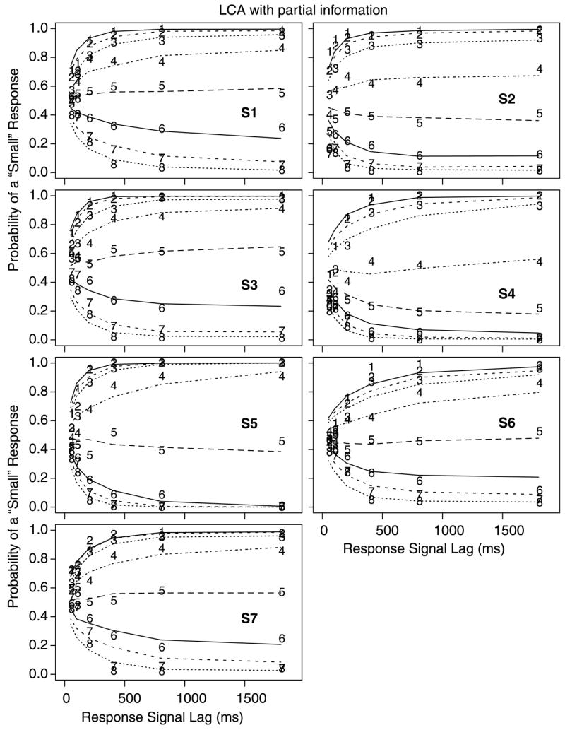
For the response signal task, Figs. 4 and 5 show the data for each of the seven subjects along with the best fits to the data for the partial information diffusion and LCA models, respectively. The numbers 1–8 on the figure show the data points for the eight groups of stimuli (1 for the smallest number of dots and 8 for the largest). The lines represent the fits of the models. The figures display the changes in probability of a “small” response across response signal lags, with the asymptotic probability highest for the conditions with the smallest numbers of dots and lowest for the conditions with the largest numbers of dots.

Fig. 4.

Probability of “small” responses in the response signal procedure as a function of response signal lag for each of the 7 subjects. The digits 1–8 refer to the experimental conditions, namely dot groups for 13–20, 21–30, 31–40, 41–50, 51–60, 61–70, 71–80, and 81–87 dots. The lines represent the fits of the best fitting model, the diffusion model with partial information.

Fig. 5.

Probability of “small” responses in the response signal procedure as a function of response signal lag for the 7 subjects. The digits 1–8 refer to the experimental conditions, namely dot groups for 13–20, 21–30, 31–40, 41– 50, 51–60, 61–70, 71–80, and 81–87 dots. The lines represent the fits of the worst fitting model, the LCA model with partial information.

Fig. 6 shows the data for the standard RT task, with four panels for each subject (“large” and “small” responses for the speed and accuracy conditions). The data are shown in quantile probability plots. For each plot, the .1, .3, .5 (median), .7, and .9 quantiles of the RT distribution for each of the eight experimental conditions are plotted as a function of response probability (except that for a few subjects/conditions, there were too few responses to compute quantiles, in which case only seven conditions are shown). The x’s are the data points and the o’s and the lines are the best fitting functions from the diffusion model with partial information. For each subject, the left-hand figures show the data for “large” responses and the right-hand figures, the data for “small” responses. As the figures show, the probability of a “large” response varies across the eight conditions from near 1 for stimuli with large numbers of dots to near 0 for stimuli with small numbers of dots, and vice versa for the probability of a “small” response. RT becomes longer for the conditions with intermediate numbers of dots, with most of the slowing coming from skewing of the RT distributions (especially from the .9 quantile RTs). Generally, across subjects, “large” responses to “large” stimuli and “small” responses to “small” stimuli are a little slower than “large” responses to “small” stimuli and “small” responses to “large” stimuli (this would correspond to error responses being faster than correct responses if this task had correct versus incorrect alternatives instead of probabilistic feedback). The advantage of quantile probability functions over other ways of displaying the data is that they contain information about all the data from the experiment: the probabilities of correct and error responses and the shapes of the RT distributions for both correct and error responses.

Fig. 6.

Quantile probability functions for “large” and “small” responses for speed and accuracy conditions for the 7 subjects. The vertical columns of x’s for each of the 8 conditions are RTs for the .1, .3, .5, .7, and .9 quantiles from lowest to highest (with only 7 columns when the extreme error condition had too few responses to compute quantile RTs). The x’s are the data and the o’s are the predicted quantile RTs from the best fitting diffusion model with partial information, joined with lines.

7.5. Model fits

Both the partial information and the guessing versions of the diffusion model fit the data better than either version of the LCA model, with the diffusion model with partial information providing a slightly better fit than the diffusion model with guessing. Table 1 shows values for the chi-square statistics for each subject for each of the four models, and G-square and BIC statistics averaged over subjects. As the chi-square and G-square statistics show, the LCA models fit more poorly than the diffusion models by about 33 and 57%, for the guessing and partial information models, respectively (note that for a perfect fit, these statistics would be zero, but BIC would be a nonzero constant). The discrepancy between the diffusion and LCA models would be reduced if the best fitting version, partial information or guessing, for each individual subject was selected for comparison, but my bias is to think that all subjects would use the same process in performing the response signal task, i.e., they would all use either partial information or they would all use guessing.

Table 1.

Chi square values for fits to individual subject data

Model and data	χ2 Values for subjects							Mean χ2 value	Mean G2 value	Mean BIC value	df
	1	2	3	4	5	6	7
Diffusion: partial, fit to joint data	409	494	459	365	424	289	505	421	445	31789	116
Diffusion: guess, fit to joint data	406	557	468	324	424	297	503	425	446	31799	115
LCA: partial, fit to joint data	625	598	679	845	605	513	761	661	663	32022	114
LCA: partial, fit to joint data (different minimum starting points)	580	522	679	667	563	518	721	607	640	32041	112
LCA: guess, fit to joint data	443	1019	560	472	422	414	598	561	537	31909	113
Diffusion: RT data alone	350	428	375	272	374	199	395	341			61
LCA: RT data alone	353	389	423	297	271	202	413	335			59
Diffusion partial; contribution from RT for fit to joint data	355	435	386	293	378	209	406	351
Diffusion guess; contribution from RT for fit to joint data	355	446	394	285	387	239	424	361
LCA partial; contribution from RT for fit to joint data	474	406	482	364	375	248	495	406
LCA partial, contribution from RT for fit to joint data (different minimum starting points)	405	366	467	398	384	251	438	387
LCA guess; contribution from RT for fit to joint data	346	510	447	383	265	272	443	381
Diffusion partial with no boundaries	741	893	968	913	852	502	856	818
LCA partial with no boundaries	710	827	978	903	753	573	807	793

The fits for the joint data from the two tasks can be examined in more detail by looking at the contributions from each task separately. Table 1 shows goodness of fit values from fitting the RT task alone and also the contributions to the chi-square values from the RT data for the joint fits. If the models fit the RT data in the joint fits in the same way as they fit the RT data alone, then the contribution to the chi-square values from the RT portion of the fit to the joint data should be about the same as the chi-square values for the fit to the RT data alone.

Table 1 shows that this is true for the diffusion model but not for the LCA model. Inspection of the chi-square values shows that the values for the RT portion of the data alone increase to the values for the joint RT—response signal data by only about 3% for the diffusion model with partial information and about 6% for the diffusion model with guessing, compared to about 21% for the LCA model with partial information and about 14% for the LCA model with guessing. This shows that for both variants of the diffusion model, the parameters for fits to the RT data alone are highly consistent with those for the joint fits. But for the LCA variants, there is distortion in the parameter values. The relative quality of the fits of the diffusion and LCA models to the RT data alone replicates what has been found before, that the two variants fit data from standard RT tasks about equally well (Ratcliff & Smith, 2004).

7.5.1. The diffusion model

The diffusion model with partial information fit the data only slightly better than the diffusion model with guessing. The goodness of fit values in Table 1 for the two models are not sufficiently different for them to be discriminated.

Fig. 4 shows the fits of the diffusion model with partial information to the response signal data for each subject. There are few deviations between the model’s predictions and the data points. The model captures both the rapid rise in accuracy and the asymptotic values of accuracy.

Fig. 6 shows the fits of the diffusion model with partial information to the data from the standard RT paradigm. Subjects 4, 5, and 6 had only three sessions of data and they show the worst fits (the value of N shown for each subject refers to an approximate number of observations per condition, the number of correct responses plus the number of error responses).

Fits of the model to accuracy data are represented by the alignment of the experimental and predicted values (the x’s and the o’s, respectively) on the x-axis in Fig. 6. In general for Subjects 1, 2, 3, and 7, the predicted and empirical values line up within about 5%. Across the data from the RT task with speed instructions and with accuracy instructions and the response signal data, the relative difficulties of the eight conditions are consistent. Accuracy is a little better (typically 4–8%) with accuracy instructions than with speed instructions.

The predictions for the RT data from the RT task match the data except for the .9 quantile RTs for some of the subjects with accuracy instructions, specifically, Subjects 2 and 5 for both “large” and “small” responses and to a lesser extent, Subjects 1 and 7 for “large” responses. With speed instructions, the data were well fit for all subjects.

Rinkenauer, Osman, Ulrich, Muller-Gethmann, and Mattes (2004) have provided electrophysiological data that suggest that speed versus accuracy instructions may produce differences in processes other than the decision process. In the diffusion and LCA models, this would produce differences in T_er between the two tasks. For Subjects 2 and 5, allowing T_er to take on different values for speed and accuracy instructions (increases of 33 and 23 ms for accuracy relative to speed for the two subjects, respectively) improved the quality of the fits by one third (chi-square values reduced from 499 and 424 to 364 and 260, respectively) and improved the visual fits, especially with accuracy instructions. All the quantiles were well fit except for the .9 quantile RTs which missed by about half as much as shown in Fig. 6. For the other subjects, allowing T_er to vary led to little improvement in fits, with chi-square values improving by less than 3% and the two values of T differing by less than 11 ms.

Tables 2 and 3 show the best fitting parameter values for the two versions of the diffusion model. There were small differences in parameter values between the chi-square and G-square fits, but generally they were only in the 0–5% range (unless the value was near zero). One larger difference was in drift rates, but the absolute differences (around .03) were compensated by an equivalent change in drift criterion so that the differences between pairs of drift rates across conditions were less than .01. Thus, although chi-square and G-square are asymptotically equivalent, the fits did not produce identical parameter values, but they were close and the qualities of the fits were equivalent.

Table 2.

Mean parameters for the diffusion models

Model	Task	a	z	sz	Ter (s)	st (s)	η	Guess prob. (“small” response)
Diffusion with partial information	Signal	0.212	0.099	0.150			0.020
	Speed	0.059	0.031	0.047	0.332	0.100
	Accuracy	0.079	0.040
Diffusion with guessing	Signal	0.118	0.070	0.021			0.049	0.406
	Speed	0.060	0.031	0.051	0.335	0.105
	Accuracy	0.080	0.041

Table 3.

Mean drift rates and accumulation rates for the diffusion models and leaky competing accumulator models

Model	v1	v2	v3	v4	v5	v6	v7	v8	Drift criterion on response signal trials
Diffusion partial	0.481	0.394	0.275	0.118	−0.019	−0.164	−0.287	−0.359	0.020
Diffusion guess	0.504	0.416	0.300	0.146	−0.007	−0.180	−0.315	−0.391	−0.059
LCA partial	0.869	0.803	0.722	0.597	0.462	0.323	0.221	0.149	0.015
LCA guess	0.995	0.948	0.811	0.658	0.494	0.314	0.212	0.147	−0.026

Note that the drift and accumulation rates are estimated for the regular RT conditions and the drift criterion values are added to drift rates to reflect bias differences between the two procedures.

For the parameters held constant across tasks, the values in Tables 2 and 3 show that drift rates differed over experimental conditions and that their absolute values were a little lower for the model with partial information than the model with guessing. Across trial variability in drift rate was smaller for the model with partial information than the model with guessing.

The parameter values that were free to vary across the response signal task and the RT task with speed instructions and with accuracy instructions behaved as expected. The main change across tasks was in boundary separation (the boundary position a, starting point z, and variability in starting point, s_z). There was greater separation in the RT task with accuracy instructions than with speed instructions, and greater separation in the response signal task than the RT task. For the response signal task, the difference in the values of the boundary separation parameters between the model with partial information and the model with guessing occurred because the model with partial information can take advantage of the greater than chance accuracy from nonterminated processes at the earliest lags (see Fig. 2, Ratcliff, 1988). In the guessing model, partial information is not available and the rise in accuracy across the earliest lags must come from terminated processes, which means the boundaries must be closer together.

7.5.2. The LCA model

The worst fitting of the models tested was the LCA model with partial information; its fits to the response signal data are shown in Fig. 5. The LCA model with guessing fit only about 15% better. Neither of the LCA models could capture the rapid rise in accuracy for the response signal data while simultaneously fitting the data from the standard RT task.

The LCA model has somewhat more flexibility than the diffusion model because, whereas in the diffusion model, the effect of moving a response boundary toward the starting point is the same as the effect of moving the starting point toward the boundary, in the LCA model, the effect of moving a response criterion closer to the starting point is not the same as moving the starting point above zero. This is because in the LCA model, the effects of decay and inhibition are greater the further the amount of accumulated information is away from the starting point.

For the partial information LCA model, I tested three variants. In the first, it was assumed that the starting points for the two criteria were constrained to have the same range (s_z) with the start of the range at zero. This model could not produce any bias at the shortest signal lags toward one or the other of the responses (e.g., the bias toward “large” responses shown by Subject 4). The predicted response signal functions were all essentially symmetric, spreading out from a starting point of about .5. This version of the LCA model produced chi-square values about 50% larger than for the best fitting diffusion model.

For the second variant of the partial information LCA model, the range of starting points was still equal for the two criteria but the minimum possible values were allowed to be larger than zero and different from each other. This variant fit better, because it allowed bias at early response lags; it reduced chi-square values to only about 30% worse than the diffusion models.

For the third variant, the decision rule for the partial information model was changed by making the winner the process nearest its criterion rather than the one that had the most accumulated information. This variant fit considerably worse than the others because of difficulty in fitting biases toward one or the other of the responses. With different starting points and different criteria for the two accumulators, and the decision rule for partial information choosing the accumulator with the most information, the starting points can be used to account for biases at short response signal lags (such as that shown by Subject 4) and the criteria can be used to account for biases at longer lags (which are mostly terminated processes). With the decision rule changed to the accumulator closest to its criteria, biases could be attributed only to the criteria, which led to poor fits (which are not shown in Table 1).

Table 4 shows parameters for the best fits of the partial information LCA model with the minima of the ranges of the starting points at zero and the guessing LCA model. The behaviors of most of the parameters were similar to those of the diffusion model. For example, the boundary separation parameters showed much wider separation for the response signal task for the partial information model than the guessing model. However, the accumulation rate parameters differed between the guessing and partial information LCA models, even when the accumulation rate criterion parameter was taken into account. The guessing model required higher accumulation rates than the partial information model.

Table 4.

Mean parameters for the leaky competing accumulator models

Model	Task	Criterion 1	Criterion 2	sz	k	β	σ	Ter (s)	st (s)	Guess prob. for a “small” response
LCA with partial information	Signal	2.053	1.934	0.646	1.002	0.250	0.502
	Speed	0.715	0.645	0.424				0.317	0.089
	Accuracy	0.900	0.827
LCA with guessing	Signal	1.238	1.164	0.566	0.885	0.260	0.477			0.533
	Speed	0.697	0.678	0.495				0.322	0.093
	Accuracy	0.869	0.876

7.6. Response signal fits with no response boundaries

The diffusion model for the response signal procedure presented by Ratcliff (1978) assumed that all decisions are based on partial information, that is, that there are no response boundaries. When a response signal is presented, a decision is based on whether the process is above or below the starting point, according to Eq. (5). A critical feature of this equation is that the growth of accuracy is determined by the ratio of the standard deviation in drift across trials and the standard deviation in drift within trials (s/η). For the standard RT task, errors slower than correct responses come from variability in drift across trials. Thus, in this version of the diffusion model, the growth of accuracy in the response signal paradigm is linked to the relative speed of correct and error responses in the standard RT paradigm. If there is a large amount of variability across trials in drift rate (e.g. Ratcliff & Rouder, 1998), then error RTs will be predicted to be long and from Eq. (5), the growth in the response signal function will be slow. With data from the same subjects for both paradigms, this prediction can be tested by using the diffusion model without boundaries for the response signal data. (For the dots paradigm, “errors” are “large” responses to small numbers of dots and “small” responses to large numbers of dots.) Note that this test is not as straightforward as directly relating the growth of accuracy to slow versus fast errors, because d′ is also determined by η, because d′_asy = (v₁ − v₂)/η.

In all the fits already reported, this version of the diffusion model was implicitly tested because the fits to the response signal data could have been achieved with decision boundaries set so wide that no processes would have terminated even at the longest response signal lag. The fitting programs did not set the boundaries this wide, and in fact, by the longest signal lag, almost all processes had already terminated and most responses were based on a decision already made. Nevertheless, we decided to see how much worse the fit was without decision boundaries.

The model was fit to the response signal and standard RT data simultaneously with response signal decisions based entirely on partial information, i.e., without decision boundaries (the guessing model without boundaries would produce only guesses so d′ would be zero). Because there were no boundaries for the response signal data, it was possible to explicitly integrate over the uniform distribution of starting points. The equation for this involved the difference between two error functions (closely related to the cumulative normal distribution functions) that have no closed form solutions but do have simple numerical solutions (not shown here). The fit was considerably worse than the fits of any of the other models. The chi square values for the fits to individual subjects are shown in Table 1 and the average goodness of fit chi-square value was twice as large as that for the diffusion model with boundaries. Almost all the increase in chi-square was the result of poorer fits to the response signal data.

The fit was so poor because, for the lower accuracy conditions, the rise of accuracy was much slower in the model than the data and the asymptotic values were much larger. This occurred because, to fit the data from the standard RT task, the value of η had to be small (because error RTs were short which requires a small value of variance in drift across trials, see Ratcliff & Rouder, 1998). This predicted too large asymptotes for the lower accuracy conditions (because asymptotic d′ is a difference in drift rates divided by η). As a result of the slower rise in accuracy, the model did not fit accuracy values at the 50 ms response signal lag; the model predictions were more extreme than the data (e.g., for conditions with positive drift rate, the predicted accuracy values at the 50 ms lag were much higher than the observed data).

For completeness, the partial information LCA model without decision boundaries was also fit to the data. The mean chi-square value (shown in Table 1) was about the same as that for the diffusion model without boundaries.

Many studies (Dosher, 1981, 1984; Gronlund & Ratcliff, 1989; McElree & Dosher, 1989; Ratcliff, 1978, 1981, 1987; Ratcliff & McKoon, 1982, 1989) have shown that the diffusion model without decision boundaries provides an acceptable account of the growth of accuracy in the response signal procedure. However, the results presented here show that it does not provide an acceptable account when it is used in simultaneously fitting response signal and standard RT data.

7.7. Relating the models to exponential fits to d′ functions

Exponential functions have often been used as a summary of response signal data, but in the introduction, I argued that they do not provide a theoretical account of processing. Furthermore, it is not possible to map the predictions of either the diffusion model or the LCA model directly onto exponential functions. For example, varying a single parameter of the diffusion or LCA model produces changes in the model’s predicted functions that can be best fit only by changing more than one parameter of the exponential. However, despite the lack of theoretical convergence between the models and the exponential function, fitting the exponential to functions generated from the diffusion and LCA models produces a reasonably good fit, and so the exponential is useful for exploring the models’ parameter spaces and could be useful in providing an empirical summary of the data as long as the parameters of the exponential are not identified with features of processing (at least not without further theoretical development). The effects of variations in model parameter values can be easily summarized by examining their effects on the parameters of the exponential. For all of the results described in this section, diffusion model with partial information was used to generate the theory based predictions.

To construct d′ functions, four conditions of the experiment were used. For fitting an exponential to the experimental data, the probabilities of a “small” response in conditions 2, 3, and 4 (moderately small numbers of dots) were used as the hit rates for these three conditions and the probability of a “small” response for condition 7 was used as the false alarm rate for all three conditions. These conditions had values of probability that were not too extreme and thus were more reliable than conditions 1 and 8. The top right panel of Fig. 7 shows that an exponential function Eq. (1) fits the data well. τ was held constant across the three conditions (the best fitting value was 313 ms) and the time intercept was set at zero (T₀ = 0). The asymptotic d′ values were 4.34, 3.80, and 2.88 for the three conditions, respectively (Table 5).

Fig. 7.

The top right panel shows fits of the exponential growth function to the average data from the experiment with d′ values obtained by scaling conditions 2, 3, and 4 against condition 7. The top left panel shows the fit of the exponential growth function to predictions from the diffusion model with the parameters from Tables 2 and 3. The middle panels show the effects of altering boundary separation for the diffusion model with partial information. The effects on the exponential growth function fit to predictions from the model are shown as a function of boundary separation, with other parameters set at the values in Tables 2 and 3. The bottom panels show the relative amounts of information for terminated processes and nonterminated processes at time T as a function of boundary separation.

Table 5.

Time constants and asymptotic d′ values for fits of exponential function to three sets of predictions for d′ as a function of time for the partial information diffusion model

Parameter and condition	One rate and three asymptotic d′ values				Three rates and three asymptotic d′ values
	τ	$d_1^{\prime }$	$d_2^{\prime }$	$d_3^{\prime }$	$d_1^{\prime }$	${\tau }_1^{\prime }$	$d_2^{\prime }$	τ2	$d_3^{\prime }$	τ3
Baseline (a = 0.212)	313	4.34	3.80	2.88	4.23	281	3.84	327	3.02	378
a = 0.106	119	2.50	2.20	1.68	2.46	109	2.21	124	1.72	138
a = 0.3	248	4.73	4.05	2.83	4.65	230	4.13	269	2.87	265
η = 0.1	278	3.83	3.26	2.39	3.78	262	3.29	289	2.44	304
sz = 0.02	278	5.87	5.05	3.73	5.76	254	5.10	291	3.86	320

Note. Predicted values of probabilities were generated from the diffusion model with partial information using the parameters in Tables 2 and 3. The hit rates from conditions 2, 3, and 4 were scaled against false alarm rates for condition 7 to produce d′ values. Exponential growth to asymptote functions were fit to the d′ functions with one time constant and three asymptotic d′ values and with three time constants and three asymptotic d′ values. The “Baseline condition” row above used the values of parameters in Tables 2 and 3 and the other rows differ only in the parameter shown (and with z = a/2 for the parameter a) from the values in Tables 2 and 3.

For the same three conditions, the top left panel shows the fits of the exponential to d′ functions generated from the diffusion model with the parameters from Tables 2 and 3 (the parameters that best fit the experimental data). Only drift rate in the diffusion model was allowed to vary across the conditions. As for fitting the data, the d′ values were constructed using the predicted probabilities of a “small” response in conditions 2, 3, and 4 as hit rates and the predicted probability of a “small” response in condition 7 as the false alarm rate. With τ held constant across the three conditions and the time intercept set at zero, the best fitting value of τ was 343 ms and the asymptotic d′ values were 4.61, 4.06, and 3.11 for conditions 2, 3, and 4, respectively.

In the fits of the exponential to values generated from the diffusion model shown in Fig. 7, only the asymptotic d′ values were allowed to vary across conditions. When τ was also allowed to vary, the fits improved; the best fitting exponentials have τ values of 281, 327, and 378 ms for conditions 2, 3, and 4 (highest d′ to lowest d′), respectively. Better fits of the exponential to the data were also achieved with τ varying across conditions. Thus, as a single parameter (drift rate) varied across the conditions for the diffusion model, there were changes in two of the exponential function parameters; large changes in the asymptotic d′ value and smaller changes in the value of τ.

Because the exponential function fits the d′ functions generated from the diffusion model well, it is possible to examine the effects of varying diffusion model parameters by looking at how they affect the exponential’s parameters. It is easier to see the effects of the diffusion model parameters on the exponential function than it is to see them by looking at the probabilities of both “large” and “small” responses across all the experimental conditions. Also, because fitting d′ values with exponential functions has been the standard method of presenting response signal data, it is easier to compare the predicted effects from the diffusion model to what is known about empirical effects.

To evaluate the effects of varying the diffusion model parameters, they were shifted from “baseline” values—the values that best fit the experimental data. The same conditions (2, 3, 4, and 7) were used as described above. To fit exponential functions to the model predictions, τ was held constant across the conditions. Although the exponential functions fit better with τ varying, the differences were not large enough to obscure the effects of interest.

The first two diffusion parameters examined were η and s_z. Increasing η, the standard deviation in drift across trials, from the value that best fit the experimental data, 0.02, to 0.1 produced modest decreases in τ, from 343 to 278 ms, and somewhat larger decreases in asymptotic d′ values, from 4.61, 4.06, and 3.11 to 3.83, 3.26, and 2.39 for conditions 2, 3, and 4, respectively. Reducing the range of the starting point, s_z, from the value that best fit the experimental data, 0.150, to 0.02, τ was reduced to 278 ms and the asymptotic d′ values were increased to 5.87, 5.05, and 3.73. In other words, overall, modest changes in variability in drift and starting point across trials have only modest effects on the rate of growth of accuracy and asymptotic accuracy. In comparison, boundary separation had large effects, as shown in the next section.

Parenthetically, note that the modest effect of changes in variability in drift across trials on the rate of growth of accuracy and asymptotic accuracy for the diffusion model with boundaries contrast with much larger effects for the model without boundaries (Ratcliff, 1978). Without boundaries, varying η from 0.02 to 0.1 leads to a decrease in τ by a factor of 10 and a decrease in asymptotic d′ by a factor of 3.

7.8. Effects of decision criteria settings on response signal performance

In the response signal paradigm, subjects must choose how to set parameters representing components of processing that are under their control so as to achieve a reasonable balance between the rate of growth of accuracy and asymptotic accuracy. Most advantageous would be a fast rate of growth to ensure accuracy at short response signal lags and a high value of asymptotic accuracy. However, in the diffusion and LCA models, there is a tradeoff between these two goals.

The parameters that have large effects on τ and asymptotic accuracy are the boundary separation parameters in the diffusion model (a and z) and the two decision criterion parameters in the LCA model (c₁ and c₂). The diffusion model with partial information is discussed first.

The middle three graphs in Fig. 7 show how asymptotic d′ and τ vary as boundary separation varies for conditions 2, 3, and 4 (which have relatively high, medium, and low asymptotic d′ values). The values of asymptotic d′ and τ that are plotted are the values for the best fits of the exponential to d′ values generated from the diffusion model. The drift rates for the three conditions were set at the values in Table 3. z was fixed at a/2 and a was varied as shown on the x-axis; 0.212 was the best fitting value of a for the experimental data and the best fitting value of z was almost a/2. The variation in asymptotic d′ and τ with boundary separation depends on the amount of variability in drift rate across trials. For the left panel, η was 0.02, the best fitting value for the experimental data, and it was increased for the other two panels. All the other parameters of the model were held constant at their best fitting values.

With η at 0.02, increasing boundary separation leads to increasing asymptotic accuracy and increasing τ, both approximately linearly over the range 0.15–0.3. The reason for these increases is illustrated in the bottom panel of Fig. 7. Response times and accuracy are shown for one condition, for which there is a large positive value of drift rate (toward a “large” response, the arrow in the figures). The areas of the distributions to the left of time T represent terminated processes and the areas to the right of T represent nonterminated processes. The black areas represent the portions of the distributions for which “large” is the response and the white areas, the portions for which “small” is the response (for the value of v in the graphs, “small” would almost certainly be an incorrect response). With narrow boundary separation (the leftmost panel), many processes have terminated, and a large proportion of them are “large” responses, so the growth of accuracy is relatively fast but asymptotic accuracy is relatively low. Also, the accuracy of the nonterminated processes is about at chance. With a medium value of boundary separation, fewer processes have terminated so the growth of accuracy is slower and asymptotic d′ is higher. Also, nonterminated processes are more accurate. Finally, with the widest separation between boundaries (the rightmost panel), very few processes have terminated so the growth of accuracy is slow, the accuracy of nonterminated processes is high, and asymptotic accuracy is high.

For the dot signal detection task used in the experiment in this article, across trial variability in drift rate was low, the 0.02 value for the leftmost of the middle panels in Fig. 7. Given this low variability, subjects had to adopt a tradeoff: they had to adopt a value of boundary separation that determined the rate of growth of accuracy and asymptotic accuracy. They chose a value of 0.212, which gives mid-range values for rate of growth and asymptotic accuracy. This produces the following proportions of terminated processes: at the 200 ms response signal lag, for condition 2, about 50% of decision processes have terminated and for condition 4, about 20% have terminated; at the 400 ms lag, about 90% have terminated for condition 2 and about 40% for condition 4.

The other two of the middle row of panels in Fig. 7 show what happens with increasing amounts of across trial variability in drift rate, 0.10 and 0.20. With 0.10, the increases with boundary separation for τ and asymptotic accuracy are slower than with 0.02. 0.20 is a value typical of recognition memory experiments (e.g., Ratcliff et al., 2004). In this case, both τ and asymptotic accuracy grow from a = 0.1 to a = 0.212, but then they start to level o. and growth is modest.

The LCA model with partial information behaves in much the same way as the diffusion model with partial information. With the parameters of the model set to those in Table 4, the best fitting values for the experimental data, varying decision criteria settings results in functions for τ and asymptotic accuracy that are within 20% of those for the diffusion model in the leftmost of the middle row of panels. The rises in the functions are approximately linear as they are for the diffusion model. The only major difference in predictions between the diffusion and LCA models is that with large variability in drift across trials (e.g., 0.20), the τ and asymptotic accuracy functions bend at about 0.212 for the diffusion model whereas the LCA model can only produce increasing functions like those in the leftmost panel of the middle row. For the LCA model, allowing the time constants to vary across experimental conditions produced time constants that differed little across conditions.

The versions of the diffusion and LCA models with guessing instead of partial information show the same general trends, although to achieve equivalent levels of accuracy, the boundaries of the models must be much closer to the starting points.

7.9. RTs in the response signal procedure

Both the diffusion and the LCA models, in both their partial information and guessing variants, can accommodate RTs in the response signal task (the times from signal presentation to response). The main assumption is that RTs for decision processes that have terminated prior to the signal are shorter than RTs for processes that have not terminated, because if a process has terminated, a subject is simply waiting for the signal.

To fit the models to the RTs, the proportion of responses of each type, terminated and nonterminated, for each lag was determined from the best fits of the models to the data. The simplest possibility is that the RTs for the two types of responses are constant across lags; all that changes is their relative proportions. However, under this assumption, the best fits significantly missed the empirical RTs, by up to 30 ms at the intermediate lags.

The assumption that allowed the models to fit the data was that RTs for nonterminated processes, but not terminated processes, vary across signal lags. The motivation for this was that, if a subject is simply waiting for the signal, then the lag between stimulus and signal is irrelevant to RT. If the decision process has not terminated, then at the signal, the process must be terminated and a response initiated, and the suggestion from other literature (cf., Pashler, 1994) is that the time required decreases with signal lag. Assuming a constant value for the RT for terminated processes of 213 ms and variable RTs for nonterminated processes allowed the models to predict the empirical RTs within 2 ms at all lags (Fig. 8). The RTs for the nonterminated processes were 270, 250, 225, 220, 213, 213 ms at the 50, 100, 200, 400, 800, 1800 ms lags, respectively.

Fig. 8.

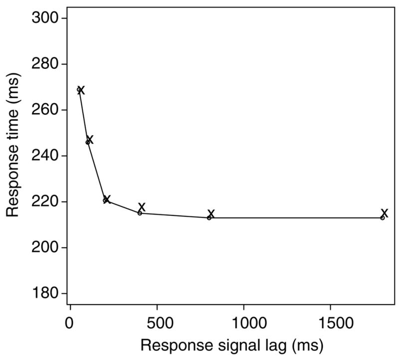
Predicted (o) and experimental (x) values of RT averaged over conditions in the response signal procedure as a function of response signal lag.

Complicating the picture of RTs in response signal paradigms is a micro-tradeoff that occurs as a function of lag: at short lags, faster responses are less accurate, whereas at long lags, faster responses are more accurate (Corbett & Wickelgren, 1978; Hintzman, Caulton, & Curran, 1994). Fig. 9 shows this tradeoff for the data from the experiment presented in this article, for four conditions with accuracy above chance but not at ceiling. At the shortest two lags, the fastest responses are the least accurate whereas at the longest three lags, the fastest responses are the most accurate.

Fig. 9.

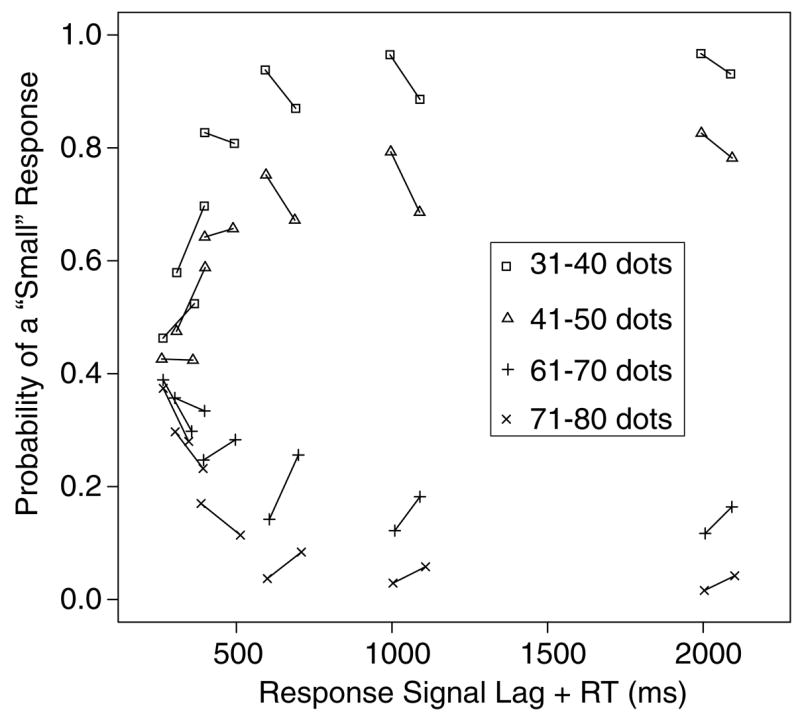
Micro-tradeoff functions for conditions with 31–40, 41–50, 61–70, and 71–80 dots in the experiment. The connected points show the accuracy of the fastest and slowest halves of the data for each condition and these are plotted as a function of response time plus signal lag.

The models can accommodate the micro-tradeoff because there is variability in processing time from stimulus onset to the signal to respond. Given this variability, then some processes will have accumulated evidence for a longer time before the response than others. At short lags, the processes that accumulate information longer will produce more accurate responses. In the partial information variants of the models, more information will be available leading to more accurate responses, and in the guessing variants, more processes will have terminated leading to more accurate responses. At longer lags, responses will be a mixture of mainly accurate terminated processes and a smaller number of less accurate nonterminated processes or guesses (see Ratcliff, 1988). Thus the models predict that at short lags, faster responses will be less accurate than slower responses, and at long lags, faster responses will be more accurate than slower responses, in accord with the data in Fig. 9.

Assuming that the time from signal to response is variable at each signal lag means that the time available to the decision process is variable. In fitting the models to the probabilities of “large” and “small” responses (Figs. 4 and 5), variability was not assumed. Adding variability would require ancillary assumptions about the distributions of times taken up by the decision process, for terminated and for nonterminated processes, perhaps different distributions at each signal lag. However, adding these types of variability to the models would not significantly change their predictions for the probabilities of “large” and “small” responses across signal lags. Also, there are not enough constraints from the data to provide a strong quantitative test of these assumptions. Nevertheless, the models can account for the micro-tradeoffs in the data qualitatively.

8. General discussion

There were two goals for the research described in this article: first, to test whether two current sequential sampling models could simultaneously account for data from the response signal paradigm and the standard RT paradigm; and second, to explore what could be learned from response signal data in the theoretical context of models that account for how information is accumulated over time.

This research is the first in which data from both the response signal and standard RT paradigms were collected from the same subjects and models were fit to both kinds of data simultaneously. The two models tested were the diffusion model (Ratcliff, 1978) and the LCA model (Usher &McClelland, 2001), models that have provided good quantitative fits to both kinds of data separately.

Previously, the models’ accounts of how processing proceeds in the response signal task rested on the assumption that evidence from the stimulus is accumulated over time until the signal to respond. At that point, the generated response was the one for which the most evidence had been accumulated. There were no response criteria, that is, the accumulation of information never terminated no matter how long the response signal lag.

In this article, following Ratcliff (1988), it is argued that it is not reasonable to assume that decision processes in the response signal task proceed without ever terminating. Instead, it is assumed that there are response criteria just as in the standard RT task, and responses come from a mixture of processes, those that have terminated at one or the other of the criteria and those that have not. These assumptions better match the intuition that, at the longest signal lags, a subject’s response has already been chosen and the subject is simply waiting for the signal to respond. In other words, at the longest signal lags, all or almost all decision processes will have terminated. As the time between stimulus and signal decreases, a larger and larger proportion of processes will have failed to terminate. For these nonterminated processes, two possibilities were tested: either partial information (i.e., the position of the process relative to the starting point) is available and can be used to determine the response or it is not available and the response is a guess.

Both versions of the diffusion model, the one with partial information available from nonterminated processes and the one with guessing, fit the data better than either version of the LCA model. For the diffusion model, the partial information and guessing versions fit about equally well, but for the LCA model, the partial information model fit 57% worse than the partial information diffusion model and the guessing model fit about 33% worse than the guessing diffusion model. The diffusion model’s account of the data across the RT and response signal tasks was more consistent than the LCA model’s: the fits of the diffusion model for the standard RT data were about equally good whether the data were fit alone or jointly with the response signal data, whereas the fits of the LCA model were not, indicating distortions between the LCA model’s fits to the two sets of data. Overall, the diffusion model gave a better account of the data than the LCA model. However, the LCA model, especially the guessing version, was not sufficiently worse than the diffusion model that it should be ruled out of consideration in future examination of two-choice decision tasks. It is possible that for other tasks or other two-choice paradigms, it could fare better than the diffusion model.¹

Crucial to any theoretical account of data from multiple, related tasks is the issue of parameter invariance. Models must reasonably map their parameters onto components of processing and the components must behave across tasks in reasonable ways. For the dot signal detection task used in the experiment in this article, it was assumed that there is no reason for a subject’s perception of numerosity to vary between tasks. Whether the task is the standard two-choice RT task, either with speed instructions or with accuracy instructions, or the response signal task, the component of processing that represents numerosity information should behave in the same way, and the variability of the numerosity information within and across trials should behave in the same way. Other assumptions could be advanced, but then it would have to be explained why and how the information available to the decision system changes across tasks. The invariance assumed here was built into the applications of both the diffusion and the LCA models, holding drift rate and variability in drift rate invariant for the diffusion model and holding accumulation rates, decay, inhibition, and within trial variability invariant for the LCA model. The components of processing that did change across tasks were those related to decision criteria, as discussed below.

Equally as important as across-task invariance is across-condition invariance. Across the conditions within an experiment, some components of processing can reasonably vary and some cannot. In the dot signal detection task, the conditions were the various numbers of dots, which varied in the difficulty with which they could be judged “large” or “small.” For the diffusion and LCA models, the parameter that reflects the varying difficulty of information from stimuli (drift rate in the diffusion model and accumulation rate in the LCA model) was the only parameter that varied across conditions. The parameters that reflect decision criteria were not allowed to vary across conditions, under the assumption that the criteria cannot be changed during the time course of processing a stimulus. In other words, for example, the criteria could not be increased after a few ms of processing to accommodate the difficulty of the decision for mid-range numbers of dots.

Given that the components of processing that reflect stimulus difficulty cannot vary across tasks and that the components that reflect decision criteria cannot vary across levels of stimulus difficulty, the models had limited flexibility (Ratcliff, 2002). The challenge was to explain how processing differed between the standard RT task and the response signal task, under the constraints just listed and also accommodating all the features of the data: accuracy values for the response signal task, and accuracy values and RT distributions for correct and error responses for the standard RT task.

The explanation of the task differences given by the models was complex but reasonable in that it depended on decision criteria, a part of processing that can be controlled by subjects. For the standard RT task, criteria settings are well understood. Subjects need more information to make a decision when they are instructed to respond as accurately as possible than when they are instructed to respond as quickly as possible, and this is achieved in sequential sampling models by setting the decision criteria at larger values with accuracy instructions. In the diffusion model, the decision boundaries are further apart, and in the LCA model, the criteria for the accumulators have larger values.

For the response signal task, criteria setting involves a tradeoff. On the one hand, it is advantageous at short response signal lags for accuracy to rise quickly from chance, but on the other hand, asymptotic accuracy (accuracy at the longest response signal lags) should be as high as possible. As was shown in Fig. 7, the settings of the criteria determine this tradeoff, and the effects of criteria settings are, in turn, determined by the amount of variability across trials in the quality of the information available from the stimuli. With the low amount of across trial variability for numerosity information in the experiment in this article, asymptotic accuracy increases as the decision criteria are set at larger values, but the rate of growth of accuracy slows. In this situation, subjects selected moderate values for their criteria settings, according to both the diffusion model and the LCA model.

The understanding of performance in the response signal procedure that is provided by the simultaneous application of the models to standard RT data and response signal data is substantially different from previous views. Older applications of the models assumed that all responses in the response signal task were based on partial information, that is, on processes that never terminated at response criteria. However, once standard RT data must be explained simultaneously with response signal data, the models with this assumption fail to fit the data.

Instead, responses in the response signal task are based on a mixture of processes that have terminated at a response criterion and processes that have not terminated. As the time between stimulus and response signal increases, the proportion of terminated processes grows and therefore accuracy grows. It may be that it is only terminated processes, plus guessing, that contribute to the growth of accuracy over time. Two versions of the models were fit to the data, one for which partial information, i.e. the position of the decision process, is available to determine the response choice, and one in which it is not and the choice is made by guessing. Both versions fit the data reasonably well, although the somewhat better fit of the guessing version of the LCA model over the partial information version might be argued against the availability of partial information to decision processes for the LCA model.

A key feature of this new interpretation of performance in the response signal task is that decision processes can terminate without subjects making an immediate response. At long response signal lags, a large proportion of decisions will already have been made and subjects simply wait for the signal. A similar situation arose in application of the diffusion model to the go–no go task. Gomez, Perea, and Ratcliff (2006) used the model to simultaneously account for lexical decision data from the standard RT paradigm and the go–no go paradigm. In the latter case, subjects were required to generate a response if the test letter string was a word but to withhold responding if it was a nonword (or vice versa). It had been suggested previously (Smith, 2000; Sperling & Dosher, 1986) that subjects set a single criterion for responding in the go–no go task. For example, if they were required to make a response if the letter string was a word, the single criterion would be set for a “word” response, and if the amount of accumulated information reached this criterion, a response would be generated. However, Gomez et al. showed that the diffusion model with only one response boundary could not fit jointly fit both the standard two-choice RT data and go–no go data from their experiments. Instead, the best fitting model was one which assumed two response boundaries, one for words and one for nonwords. In the standard RT task, responses were generated when the amount of accumulated information reached either boundary. In the go–no go task, responses were generated only when the amount of accumulated information reached the boundary assigned to the “go” response. When the amount of accumulated information reached the boundary assigned to the “no-go” response, subjects simply waited for the next trial. The across-task assumptions about parameter invariance were the same for this pair of tasks as for application of the model to the standard RT and response signal tasks, namely that the difficulty of the decision presented by a stimulus should not change across tasks. For the Gomez et al. data, the drift rates for high and low frequency words did not change between their two tasks; instead, just as with the standard RT and response signal data in this article, response criteria changed. Thus there is theoretical convergence between the application of the diffusion model in this article and in Gomez et al.; in both cases it is assumed that processes terminate without an immediate explicit response and it is assumed that some parameters of processing are invariant across tasks.

8.1. Other approaches to the response signal procedure

The traditional approach to fitting data from the response signal procedure has been to convert the probabilities of responses at each response signal lag to d′ values by scaling against one baseline condition and fitting an exponential growth to asymptote function to d′ functions. The parameters of the exponential (the asymptotic d′ level, the rate of growth, and the delay before the function begins to grow above chance) are then used to interpret performance. However, the exponential does not have grounding in a process model and should be viewed only as providing a summary of empirical data and a target for process models to fit.

In another approach, Wagenmakers et al. (2004) proposed that response signal data for lexical decision could be explained by an extension of the REM memory model (Shifirin & Steyvers, 1997). The REM model provides values of how wordlike letter strings are, and along with an assumption of exponentially distributed feature availability overtime, the model was used to fit probabilities of “word” and “nonword” responses as a function of response signal lag. However, only response signal data were fitted; there was no attempt to simultaneously fit response signal data and the standard RT task. Wagenmakers et al. speculated that their REM extension to response signal data could be combined with a random walk model for standard RT data (e.g. Laming, 1968; Link & Heath, 1975; Stone, 1960). However, successfully fitting data with a combination of the REM extension, which has no response boundaries or criteria, and a random walk model that does have response boundaries is likely to be difficult.

9. Conclusions

The first conclusion is that applying models to multiple tasks simultaneously produces powerful constraints on the models that (if the models can successfully account for the data) lead to new understandings of how the tasks are performed. Here, in the context of sequential sampling models, this approach yielded a new view of response signal performance: responses increase in accuracy over time mainly because the proportion of terminated processes increases; the increase in accuracy does not come entirely from the increasing availability of partial information. Moreover, applying the models to the standard RT procedure and the response signal procedure simultaneously showed that there are versions of the models that can fit the data well for the response signal procedure individually but not for both procedures simultaneously.

The second point is that, although exponential functions give good fits to d′ values as a function of signal lag, they do not provide a model of underlying cognitive processes, nor do the parameters of the exponential correspond directly to the components of processing in either the diffusion or the LCA models. For example, differences across experimental conditions in asymptotic d′ values, as determined by fits of the exponential, do not correspond directly to drift rates or accumulation rates. However, exponential functions do provide concise and useful summaries of the data.

Finally, under the new explanation of response signal performance, accuracy is determined in part by the decision criteria settings adopted by subjects, just as accuracy and RT are determined by criteria settings in the standard RT task. However, despite being under the control of subjects’ criteria settings, the procedure is still valid for the research questions to which it is typically applied. As long as subjects can be assumed to hold their response criteria constant across experimental conditions, then differential increases in response accuracy over time between one condition and another reflect differences in the proportions of terminated processes (and possibly the accuracy of nonterminated processes) —in other words, differences in the amount of information available from the stimuli.

References

- Ashby FG. A biased random walk model of two choice reaction times. Journal of Mathematical Psychology. 1983;27:277–297. [Google Scholar]
- Ashby FG, Gott RE. Decision rules in the perception and categorization of multidimensional stimuli. Journal of Experimental Psychology: Learning, Memory, and Cognition. 1988;14:33–53. doi: 10.1037//0278-7393.14.1.33. [DOI] [PubMed] [Google Scholar]
- Busemeyer JR, Townsend JT. Decision field theory: A dynamic-cognitive approach to decision making in an uncertain environment. Psychological Review. 1993;100:432–459. doi: 10.1037/0033-295x.100.3.432. [DOI] [PubMed] [Google Scholar]
- Corbett AT, Wickelgren WA. Semantic memory retrieval: Analysis by speed–accuracy tradeoff functions. Quarterly Journal of Experimental Psychology. 1978;30:1–15. doi: 10.1080/14640747808400648. [DOI] [PubMed] [Google Scholar]
- De Jong R. Partial information or facilitation? Different interpretations of results from speed–accuracy decomposition. Perception & Psychophysics. 1991;50:333–350. doi: 10.3758/bf03212226. [DOI] [PubMed] [Google Scholar]
- Dosher BA. The retrieval of sentences from memory: A speed–accuracy study. Cognitive Psychology. 1976;8:291–310. [Google Scholar]
- Dosher BA. Empirical approaches to information processing: Speed–accuracy tradeoff functions or reaction time. Acta Psychologica. 1979;43:347–359. [Google Scholar]
- Dosher BA. The effects of delay and interference on retrieval dynamics: Implications for retrieval models. Cognitive Psychology. 1981;13:551–582. [Google Scholar]
- Dosher BA. Effect of sentence size and network distance on retrieval speed. Journal of Experimental Psychology: Learning, Memory, and Cognition. 1982;8:173–207. [Google Scholar]
- Dosher BA. Discriminating preexperimental (semantic) from learned (episodic) associations: A speed– accuracy study. Cognitive Psychology. 1984;16:519–555. [Google Scholar]
- Espinoza-Varas B, Watson C. Effects of decision criterion on response latencies of binary decisions. Perception & Psychophysics. 1994;55:190–203. doi: 10.3758/bf03211666. [DOI] [PubMed] [Google Scholar]
- Feller W. An introduction to probability theory and its applications. New York: John Wiley & Sons; 1968. [Google Scholar]
- Gomez P, Perea M, Ratcliff R. A model of the go/no-go lexical decision task. 2006 (submitted) [Google Scholar]
- Gronlund SD, Ratcliff R. The time-course of item and associative information: Implications for global memory models. Journal of Experimental Psychology: Learning, Memory and Cognition. 1989;15:846–858. doi: 10.1037//0278-7393.15.5.846. [DOI] [PubMed] [Google Scholar]
- Heuer H. Visual discrimination and response programming. Psychological Research. 1987;49:91–98. doi: 10.1007/BF00308673. [DOI] [PubMed] [Google Scholar]
- Hintzman DL, Caulton DA, Curran T. Retrieval constraints and the mirror effect. Journal of Experimental Psychology: Learning, Memory, and Cognition. 1994;20:275–289. [Google Scholar]
- Hintzman DL, Curran T. Comparing retrieval dynamics in recognition memory and lexical decision. Journal of Experimental Psychology: General. 1997;126:228–247. [Google Scholar]
- Jeffreys H. Theory of probability. 3. Oxford: Oxford University Press; 1961. [Google Scholar]
- Kounios J, Osman AM, Meyer DE. Structure and process semantic memory: New evidence based on speed–accuracy decomposition. Journal of Experimental Psychology: General. 1987;116:3–25. doi: 10.1037//0096-3445.116.1.3. [DOI] [PubMed] [Google Scholar]
- Laming DRJ. Information theory of choice reaction time. New York: Wiley; 1968. [Google Scholar]
- Lee W, Janke M. Categorizing externally distributed by stimulus samples for three continua. Journal of Experimental Psychology. 1964;68:376–382. doi: 10.1037/h0042770. [DOI] [PubMed] [Google Scholar]
- Link SW. The relative judgement theory of two choice response time. Journal of Mathematical Psychology. 1975;12:114–135. [Google Scholar]
- Link SW, Heath RA. A sequential theory of psychological discrimination. Psychometrika. 1975;40:77–105. [Google Scholar]
- McElree B, Dosher BA. Serial position and set size in short-term memory: Time course of recognition. Journal of Experimental Psychology: General. 1989;18:346–373. [Google Scholar]
- McElree B, Dosher BA. Serial retrieval processes in the recovery of order information. Journal of Experimental Psychology: General. 1993;122:291–315. [Google Scholar]
- Meyer DE, Irwin DE, Osman AM, Kounios J. The dynamics of cognition: mental processes inferred from a speed–accuracy decomposition technique. Psychological Review. 1988;95:183–237. doi: 10.1037/0033-295x.95.2.183. [DOI] [PubMed] [Google Scholar]
- Meyer DE, Yantis S, Osman A, Smith JEK. Temporal properties of human information processing: Tests of discrete versus continuous models. Cognitive Psychology. 1985;17:445–518. doi: 10.1016/0010-0285(85)90016-7. [DOI] [PubMed] [Google Scholar]
- Nelder JA, Mead R. A simplex method for function minimization. Computer Journal. 1965;7:308–313. [Google Scholar]
- Nosofsky RM. Attention and learning processes in the identification and categorization of integral stimuli. Journal of Experimental Psychology: Learning, Memory, and Cognition. 1987;13:87–109. doi: 10.1037//0278-7393.13.1.87. [DOI] [PubMed] [Google Scholar]
- Pashler H. Dual-task interference in simple tasks: Data and theory. Psychological Bulletin. 1994;116:220–244. doi: 10.1037/0033-2909.116.2.220. [DOI] [PubMed] [Google Scholar]
- Ratcliff R. A theory of memory retrieval. Psychological Review. 1978;85:59–108. [Google Scholar]
- Ratcliff R. A note on modeling accumulation of information when the rate of accumulation changes overtime. Journal of Mathematical Psychology. 1980;21:178–184. [Google Scholar]
- Ratcliff R. A theory of order relations in perceptual matching. Psychological Review. 1981;88:552–572. [Google Scholar]
- Ratcliff R. Theoretical interpretations of speed and accuracy of positive and negative responses. Psychological Review. 1985;92:212–225. [PubMed] [Google Scholar]
- Ratcliff R. Proceedings of the ninth annual conference of the Cognitive Science Society. Hillsdale, NJ: Erlbaum; 1987. Order information and distributed memory models. [Google Scholar]
- Ratcliff R. Continuous versus discrete information processing: Modeling the accumulation of partial information. Psychological Review. 1988;95:238–255. doi: 10.1037/0033-295x.95.2.238. [DOI] [PubMed] [Google Scholar]
- Ratcliff R. A diffusion model account of reaction time and accuracy in a brightness discrimination task: Fitting real data and failing to fit fake but plausible data. Psychonomic Bulletin and Review. 2002;9:278–291. doi: 10.3758/bf03196283. [DOI] [PubMed] [Google Scholar]
- Ratcliff R, McKoon G. Speed and accuracy in the processing of false statements about semantic information. Journal of Experimental Psychology: Learning, Memory, and Cognition. 1982;8:16–36. [Google Scholar]
- Ratcliff R, McKoon G. Similarity information versus relational information: Differences in the time course of retrieval. Cognitive Psychology. 1989;21:139–155. doi: 10.1016/0010-0285(89)90005-4. [DOI] [PubMed] [Google Scholar]
- Ratcliff R, Rouder JF. Modeling response times for two-choice decisions. Psychological Science. 1998;9:347–356. [Google Scholar]
- Ratcliff R, Rouder JF. A diffusion model account of masking in two-choice letter identification. Journal of Experimental Psychology: Human Perception and Performance. 2000;26:127–140. doi: 10.1037//0096-1523.26.1.127. [DOI] [PubMed] [Google Scholar]
- Ratcliff R, Smith PL. A comparison of sequential sampling models for two-choice reaction time. Psychological Review. 2004;111:333–367. doi: 10.1037/0033-295X.111.2.333. [DOI] [PMC free article] [PubMed] [Google Scholar]
- Ratcliff R, Tuerlinckx F. Estimating the parameters of the diffusion model: approaches to dealing with contaminant reaction times and parameter variability. Psychonomic Bulletin and Review. 2002;9:438–481. doi: 10.3758/bf03196302. [DOI] [PMC free article] [PubMed] [Google Scholar]
- Ratcliff R, Gomez P, McKoon G. Diffusion model account of lexical decision. Psychological Review. 2004;111:159–182. doi: 10.1037/0033-295X.111.1.159. [DOI] [PMC free article] [PubMed] [Google Scholar]
- Ratcliff R, Thapar A, Gomez P, McKoon G. A diffusion model analysis of the effects of aging on lexical decision. Psychology and Aging. 2004;19:278–289. doi: 10.1037/0882-7974.19.2.278. [DOI] [PMC free article] [PubMed] [Google Scholar]
- Ratcliff R, Thapar A, McKoon G. The effects of aging on reaction time in a signal detection task. Psychology and Aging. 2001;16:323–341. [PubMed] [Google Scholar]
- Ratcliff R, Thapar A, McKoon G. A diffusion model analysis of the effects of aging on brightness discrimination. Perception & Psychophysics. 2003;65:523–535. doi: 10.3758/bf03194580. [DOI] [PMC free article] [PubMed] [Google Scholar]
- Ratcliff R, Thapar A, McKoon G. A diffusion model analysis of the effects of aging on recognition memory. Journal of Memory and Language. 2004;50:408–424. [Google Scholar]
- Ratcliff R, Van Zandt T, McKoon G. Connectionist and diffusion models of reaction time. Psychological Review. 1999;106:261–300. doi: 10.1037/0033-295x.106.2.261. [DOI] [PubMed] [Google Scholar]
- Reed AV. Speed–accuracy trade-off in recognition memory. Science. 1973;181:574–576. doi: 10.1126/science.181.4099.574. [DOI] [PubMed] [Google Scholar]
- Reed AV. List length and the time course of recognition in human memory. Memory and Cognition. 1976;4:16–30. doi: 10.3758/BF03213250. [DOI] [PubMed] [Google Scholar]
- Rinkenauer G, Osman A, Ulrich R, Muller-Gethmann H, Mattes S. On the locus of speed– accuracy tradeoff in reaction time: Inferences from the lateralized readiness potential. Journal of Experimental Psychology: General. 2004;133:261–282. doi: 10.1037/0096-3445.133.2.261. [DOI] [PubMed] [Google Scholar]
- Roe RM, Busemeyer JR, Townsend JT. Multialternative decision field theory: A dynamic connectionist model of decision-making. Psychological Review. 2001;108:370–392. doi: 10.1037/0033-295x.108.2.370. [DOI] [PubMed] [Google Scholar]
- Schouten JF, Bekker JAM. Reaction time and accuracy. Acta Psychologica. 1967;27:143–153. doi: 10.1016/0001-6918(67)90054-6. [DOI] [PubMed] [Google Scholar]
- Schwarz G. Estimating the dimension of a model. Annals of Statistics. 1978;6:461–464. [Google Scholar]
- Shiffrin RM, Steyvers M. A model for recognition memory: REM: Retrieving effectively from memory. Psychonomic Bulletin and Review. 1997;4:145–166. doi: 10.3758/BF03209391. [DOI] [PubMed] [Google Scholar]
- Smith PL. Psychophysically principled models of visual simple reaction time. Psychological Review. 1995;102:567–591. [Google Scholar]
- Smith PL. Stochastic dynamic models of response time and accuracy: A foundational primer. Journal of Mathematical Psychology. 2000;44:408–463. doi: 10.1006/jmps.1999.1260. [DOI] [PubMed] [Google Scholar]
- Smith PL, Vickers D. The accumulator model of two-choice discrimination. Journal of Mathematical Psychology. 1988;32:135–168. [Google Scholar]
- Smith PL, Ratcliff R, Wolfgang BJ. Attention, visual short term memory, and the representation of stimuli in psychophysical decisions. Vision Research. 2004;44:1297–1320. doi: 10.1016/j.visres.2004.01.002. [DOI] [PubMed] [Google Scholar]
- Sperling G, Dosher BA. Strategy and optimization in human information processing. In: Bo K, Kaufman L, Thomas J, editors. Handbook of human perception & performance. Vol. 1. New York: Wiley; 1986. pp. 2-1–2-65. [Google Scholar]
- Stone M. Models for choice reaction time. Psychometrika. 1960;25:251–260. [Google Scholar]
- Thapar A, Ratcliff R, McKoon G. A diffusion model analysis of the effects of aging on letter discrimination. Psychology and Aging. 2003;18:415–429. doi: 10.1037/0882-7974.18.3.415. [DOI] [PMC free article] [PubMed] [Google Scholar]
- Usher M, McClelland JL. The time course of perceptual choice: The leaky, competing accumulator model. Psychological Review. 2001;108:550–592. doi: 10.1037/0033-295x.108.3.550. [DOI] [PubMed] [Google Scholar]
- Van Zandt T, Ratcliff R. Statistical mimicking of reaction time distributions: mixtures and parameter variability. Psychonomic Bulletin and Review. 1995;2:20–54. doi: 10.3758/BF03214411. [DOI] [PubMed] [Google Scholar]
- Vickers D. Evidence for an accumulator model of psychophysical discrimination. Ergonomics. 1970;13:37–58. doi: 10.1080/00140137008931117. [DOI] [PubMed] [Google Scholar]
- Vickers D. Decision processes in visual perception. New York: Academic Press; 1979. [Google Scholar]
- Vickers D, Caudrey D, Willson RJ. Discriminating between the frequency of occurrence of two alternative events. Acta Psychologica. 1971;35:151–172. [Google Scholar]
- Wagenmakers EJ, Ratcliff R, Gomez P, Iverson GJ. Assessing model mimicry using the parametric bootstrap. Journal of Mathematical Psychology. 2004;48:28–50. [Google Scholar]
- Wagenmakers EJ, Steyvers M, Raaijmakers JGW, Shiffrin RM, van Rijn H, Zeelenberg R. A model for evidence accumulation in the lexical decision task. Cognitive Psychology. 2004;48:332–367. doi: 10.1016/j.cogpsych.2003.08.001. [DOI] [PubMed] [Google Scholar]
- Wickelgren WA. Speed–accuracy tradeoff and information processing dynamics. Acta Psvchologica. 1977;41:67–85. [Google Scholar]
- Wickelgren WA, Corbett AT, Dosher BA. Priming and retrieval from short-term memory: A speed accuracy trade-off analysis. Journal of Verbal Learning and Verbal Behavior. 1980;19:387–404. [Google Scholar]