Efficiency of DNA replication in the polymerase chain reaction

Abstract

A detailed quantitative kinetic model for the polymerase chain reaction (PCR) is developed, which allows us to predict the probability of replication of a DNA molecule in terms of the physical parameters involved in the system. The important issue of the determination of the number of PCR cycles during which this probability can be considered to be a constant is solved within the framework of the model. New phenomena of multimodality and scaling behavior in the distribution of the number of molecules after a given number of PCR cycles are presented. The relevance of the model for quantitative PCR is discussed, and a novel quantitative PCR technique is proposed.

The polymerase chain reaction (PCR) is one of the most widely used techniques in modern molecular biology. It was devised (1) as a method for amplifying specific DNA sequences (targets), and the scope of its applications stretches from medicine (2), through in vitro evolution (3), to molecular computers (4, 5). In spite of its ubiquity in biology, theoretical discussions of PCR are rare. Although kinetic models of the enzyme-mediated polymerization of single-stranded DNA have been reported (6–10), none of them were applied to model PCR, and only recently has a treatment of the rate of mutations arising in PCR been considered (11, 12).

The main object of our study is the probability that one molecule will be replicated in one PCR cycle, the so-called efficiency p. In the second section we present a detailed kinetic model of the polymerization and find p as a function of the physical parameters of the system. This allows us to discuss the range of validity of the assumption of constant probability of replication, on which statistical considerations have been based (11, 12). Within that range, we apply the theory of branching processes in the third section, Statistical Analysis, to show the existence of new phenomena: the probability density function (pdf) of the number of molecules after a given number of cycles of PCR displays scaling behavior, and under some conditions, this pdf is multimodal. In the fourth section, a novel method for quantitative PCR is presented, based on the statistical considerations of the previous sections. In the final section we summarize our work.

One cycle of PCR consists of three steps. (For a more detailed account of the PCR technique see, e.g., ref. 13.) In the denaturing step, the two strands of the parent DNA molecule in solution are separated into single-stranded (ss) templates by raising the temperature to about 95°C to disrupt the hydrogen bonds. In the annealing step, the solution is cooled down to approximately 50°C to allow the primers, present in a high concentration, to hybridize with the ssDNA. The primers are two (different) 20- to 30-nucleotide-long molecules which are Watson–Crick complementary to the 3′ flanking extreme of the templates. Once the primer-template heteroduplex is formed, it acts as the initiation complex for the DNA polymerase* to recognize and bind to. This step is crucial for the specificity of the amplification: only those molecules that have sequences complementary to the primers will be amplified. The last step is a polymerization reaction, in which the solution is heated to 72°C, the optimal working temperature for Thermus aquaticus (Taq) DNA polymerase. This enzyme catalyzes the binding of complementary nucleotides to the template, in the direction that goes from the primer to the other extreme.† Notice that if this polymerization proceeded to its end, at the end of the third step we would have twice as many DNA molecules as we had at the beginning of step 1. These three steps constitute one cycle of the PCR, which is usually 30 s to 2 min long. The cycles are repeated a number of times (typically 30) by varying the temperature in the solution, in such a way that the DNA molecules that were synthesized in a given cycle are used as templates in the following one. In this way one gets an extremely efficient amplification mechanism for DNA.

Kinetic Model

We will represent the last two steps of a typical cycle of PCR by means of a kinetic model. Our species will be the primers (pr, of length L_p nucleotides), the single-stranded DNA (ss, consisting of L_p + N nucleotides), the heteroduplexes (h_i, formed by one complete ss and the partially assembled complementary strand consisting of the primer and the next i nucleotides), the nucleotides (n, which will be considered identical), the polymerase (q), and the heteroduplexes h_i with the polymerase attached to them (qh_i). Denoting by κ_2j−1 and κ_2j the forward and backward chemical reaction rates, the chemical equations are

1

Other recognizable species might be present in the chain reaction. This can occur because of substitutions, additions, or deletions of nucleotides by the polymerase, or because of the presence of sequence-dependent structures. These will not be taken into account in our model, for the sake of simplicity. Assuming that the effects of inhomogeneities in density and temperature are irrelevant, it is well known that Eqs. 1 lead to a corresponding system of first-order nonlinear differential equations for the concentrations of the different species as functions of time, which we are not going to write here (see, for example, ref. 15). In the above reactions, one should assign a given duration to step 2 and another to step 3. For the sake of simplicity, however, we shall consider both step 2 and step 3 as running simultaneously in the simulations to be presented below. This is a mild simplification which does not alter the conclusions to be drawn.

The definition of the efficiency (or probability of replication) p implies that it is simply the ratio between the number of ss molecules that were completely replicated at the end of a given cycle and the initial number of ss molecules in that cycle:

2

Fig. 1 shows plots of the probability of replication p as a function of time t (which is to be interpreted as the duration of step 3 in a typical PCR cycle), for different polymerization lengths N. Since to the best of our knowledge the chemical reaction constants κs have not been measured for Taq polymerase, we have assumed some values for these constants to exemplify the principal characteristics of our model. It should be stressed, however, that the equivalent to some of these constants have been measured for other polymerases such as T4 phage DNA polymerase (6), T7 phage DNA polymerase (7), and Escherichia coli DNA polymerase I (Klenow fragment) (8–10). The values of the chemical reaction constants κ and the initial conditions used in the simulation of Eqs. 1 are detailed in the legend to Fig. 1. The main features of the curves in Fig. 1 can be quantitatively understood. It can be observed that the larger N, the flatter the behavior at small times. Indeed it can be shown from the dynamic equations that p ∼ t^(2N+1)/3 for t sufficiently small. The time at which p has reached about half its asymptotic value, as well as the width of the rise-time, can be estimated from a further simplification of our model. Assuming that the time constants associated with the backwards reactions in Eqs. 1 are large enough, and that the concentration of primers, polymerase, and nucleotides are sufficiently large that their relative concentrations can be considered as constants (or more precisely as slowly varying parameters) during the process, we can rewrite the reaction as

3

The time τ needed for this reaction to be completed is simply the sum of the times corresponding to each link of the chain, τ = τ_κ1 + τ_κ3 + τ_κ5,1 + … + τ_κ5,N, where τ_κ1 and τ_κ3 are the times associated with the first two reactions in Eq. 3, and τ_κ5,j is the time associated with the reaction qh_j−1^n↓κ₅→ qh_j. These τs are independent, exponentially distributed random variables, whose mean values are 〈τ_κ1〉 = (κ₁[pr])⁻¹, 〈τ_κ3〉 = (κ₃[q])⁻¹, and 〈τ_κ5,j〉 = (κ₅[n])⁻¹. Therefore, it can be readily seen that the mean and the standard deviation of τ are

4

5

where we used that the variance of an exponentially distributed random variable is the square of its mean. 〈τ〉 and σ_τ can be used as estimates of mean rise-time and the rise-time width about the mean for the complete reaction. These estimates are shown in Fig. 1. The abscissa of the solid square on each curve corresponds to the value predicted by Eq. 4, and the arrowheads indicate the values of 〈τ〉 ± σ_τ. It can be safely concluded that Eqs. 4 and 5, computed from the simplified chain reactions of Eq. 3, are good estimates of the mean rise-time and the rise-time width corresponding to the full set of reactions.

Figure 1.

Probability of replication p(t) as a function of time t, for different template lengths N (in number of nucleotides without including the primers) arising from a numerical simulation of Eqs. 1, with parameters: κ₁ = 10⁹ M⁻¹·s⁻¹, κ₂ = 10⁻² s⁻¹, κ₃ = 10⁷ M⁻¹·s⁻¹, κ₄ = 10⁻³ s⁻¹, κ₅ = 10⁷ M⁻¹·s⁻¹, κ₆ = 15 s⁻¹, κ₇ = 10⁹ M⁻¹·s⁻¹, κ₈ = 10⁻¹ s⁻¹, [pr](0) = 10⁻⁶ M, [n](0) = 10⁻⁵ M, [q](0) = 10⁻⁶ M, [ss](0) = 10⁻¹¹ M. The square and arrowheads indicate, respectively, the mean rise-time and rise-time width as predicted by the simplified model of Eqs. 3.

The last important feature to be extracted from Fig. 1 is the tendency of p(t) towards an asymptote p_∞, which corresponds to the equilibrium of the chemical system. This value is of importance in PCR, and thus it is worth computing it in terms of the parameters of our model. The detailed balance equilibrium conditions for the reactions of Eqs. 1 demand that [ss]_eq/[h₀]_eq = κ₂/(κ₁[pr]_eq) ≡ α₁, [h_i]_eq/[qh_i]_eq = κ₄/(κ₃[q]_eq) ≡ α₃ (for 0 ≤ i ≤ N − 1), [qh_i]_eq/([qh_i+1]_eq) = κ₆/(κ₅[n]_eq) ≡ α₅ (for 0 ≤ i ≤ N − 1) and [h_N]_eq/[qh_N]_eq = κ₈/(κ₇[q]_eq) ≡ α₇. On using Eq. 2 and the conservation relation [ss](t) + Σ_i=0^N {[h_i](t) + [qh_i](t)} = [ss](0), one obtains that

6

For the purpose of computing p_∞ one should know the values of [pr]_eq, [n]_eq, and [q]_eq. As an approximation to these values one can use the initial values of these species at the beginning of the cycle. This approximation will be excellent if these initial concentrations are sufficiently large. The values of p_∞ (computed under this approximation) corresponding to the conditions of the simulations of Fig. 1 are 0.87 for N = 1 and 0.85 for N = 10 and N = 45, in perfect agreement with the complete simulation. It is interesting to notice that from direct measurements of p(t) a wealth of information on the rate constants involved in the polymerization reactions can be inferred using Eqs. 4–6.

Of utmost importance in applications of PCR is the number of cycles of PCR during which the amplifying process is exponential. As will be discussed later on, the mean number of molecules 〈N_k+1〉 at cycle k + 1 is related to the mean number of molecules 〈N_k〉 at cycle k by the relation 〈N_k+1〉 = (1 + p_k)〈N_k〉, where p_k is the efficiency during the kth cycle. Therefore the rate of growth will be exponential only when p_k is independent of k. During how many cycles can the system maintain p_k constant? The answer can be found if we think that during these cycles, both the concentration of primers and nucleotides will also be decreasing exponentially, and therefore their concentration at cycle k will be [pr]_k = [pr]₀ − (1 + p)^k[ss]₀ and [n]_k = [n]₀ − (1 + p)^kN[ss]₀. The mean rise-time and rise-time width for p at cycle k, 〈τ〉_k and σ_τ,k, will be given by Eqs. 4 and 5, with [pr] and [n] replaced by [pr]_k and [n]_k, respectively. If the time for the reaction is t, then the maximum number of cycles ν during which p_k can be considered constant will be given, to a first approximation, by the ν that verifies that 〈τ〉_ν + σ_τ,ν = t. This imposes an equation for ν that can be solved numerically. An approximation to this solution is

7

where log_b indicates logarithm to the base b. Notice that as t becomes larger, the value of ν predicted in Eq. 7 tends to a constant independent of t, given by the number of cycles that it takes to deplete the solution of nucleotides or primers, whichever is exhausted first. Although it might be unrealistic for the conditions used in molecular biology, it is interesting to notice that if the nucleotides are the first species to be exhausted, then most of the heteroduplexes will cease to polymerize before reaching the end, with the outcome that there will hardly be any complete double helix formed: in this case the net amplification factor will be close to zero. Fig. 2 shows the efficiency p_k at cycle k as a function of the number of cycles, for different times of polymerization and N = 45 (the other parameters are as in Fig. 1), obtained by the integration of the reactions of Eq. 1. In this simulation we concatenated cycles, assuming a perfect melting step, which was done by hand by setting [ss]_k+1(0) in the cycle k + 1 equal to [ss]_k(0) + [h_N]_k(t) + [qh_N]_k(t) of the previous cycle and [h_i]_k+1(0) = [qh_i]_k+1(0) = 0 (0 ≤ i ≤ N). The dynamics of pr and n, on the other hand, was followed exactly. It is clear from Fig. 2 that there is a regime for which p_k is roughly constant, and that the extent of this regime tends to decrease with t. The values of ν predicted by the condition 〈τ〉_ν + σ_τ,ν = t are 13 for t = 0.8 s and 15 for t = 2.0 s (slightly overestimated by Eq. 7, whose integer part yields 14 for t = 0.8 s and 15 for t = 2.0 s), in rough agreement with the values of about 12 and 14, respectively, obtained from Fig. 2.

Figure 2.

Efficiency p_k as a function of the cycle number k, for different polymerization times. The length of the template is N = 45; the other parameters are as in Fig. 1.

At this point a few important considerations are in order. The fraction 1 − p of molecules whose replication was incomplete will give rise to incomplete complementary single strands. Only when these incomplete replicas are close to completion will they be able to bind a primer in the next cycle, and thus be replicated. Therefore the efficiency p defined in Eq. 2 is an underestimation, since h_N−1, h_N−2,…, h_N−j as well as qh_N−1, qh_N−2,…, qh_N−j (for some j < L_p, where L_p is the length of the primers) will be part of the pool of templates in subsequent cycles. However, the dominant process will be the replication of the complete strand, which justifies the computation of p as in Eq. 2. There is another issue that needs some discussion. All the complementary strands arising from both complete and incomplete replication of a template can anneal to that template in subsequent cycles, and therefore can act effectively as primers. Strictly speaking, at any given cycle k ≥ 1 there will be a pool of primers of different lengths. An estimate of the concentration of “primers” arising from incomplete replication at cycle k is ((1 − p)/p)(1 + p)^k[ss](0). This amount is always smaller than the concentration (1 + p)^k[ss](0) of completely replicated single strands which act also as potential “primers.” As long as the concentration of incomplete replicas remain much smaller than the concentration of primers [pr], Eqs. 1 will constitute a good approximation to the PCR process. Recall now that ν (see Eq. 7) is equal or smaller than the number of cycles required for the concentration of primers [pr] to match the concentration of completely replicated single-stranded molecules. It follows that the approximation given by Eqs. 1 will break down only after the number of PCR cycles is bigger than ν, and therefore our basic conclusions, contained in Eqs. 4–7, are not altered.

Statistical Analysis

As seen above, the efficiency p can be assumed to be constant for a number of cycles of PCR. The statistics of PCR can be readily computed under this assumption. The basic element in the analysis is the recursive relation that links the number of replicates after cycle number n + 1, N_n+1 in terms of N_n,

8

where B(N_n;p) is a random variable whose distribution is binomial with parameters N_n and p. The basis for this relation is that at the (n + 1)-th cycle there will be not only the N_n molecules that were present at the previous cycle but also the number of successful replication after N_n Bernoulli trials (16), each one with probability p of success. The number of molecules in the initial sample will be denoted by M₀.

The first moments of N_n can be easily computed from Eq. 8:

9

10

Furthermore, using the theory of branching processes (17, 18), a recursive relation between P_n^M₀(k) (the probability that there are k molecules at cycle n, having started with M₀ of them) and P_n−1^M₀(k) can be obtained

11

(where j_max = min {M₀2ⁿ⁻¹, k}, and [k/2] denotes the integer part of k/2), which when supplemented with the initial condition P₀^M₀(k) = δ_k,M0 allows us to compute P_n^M₀(k) for any n. Fig. 3 shows the form of these probability functions for n = 10 with M₀ = 1 in Fig. 3a, and M₀ = 50 in Fig. 3b, and different values of p. A remarkable resonance-like behavior can be observed in the curve corresponding to p = 0.9 and M₀ = 1 (wavy curve in Fig. 3a. This phenomenon originates in the discrete nature of the process: if at the first cycle the system fails in replicating the only original template, then the subsequent growth of the population will be as if there were nine cycles instead of ten. The other peaks correspond to the failure in replication in the first two cycles, three cycles, etc. This trait is characteristic of values of p between, say, 0.8 and 1. For smaller values of p the function looks smoother. A common feature of the curves in Fig. 3a is the existence of a power law regime in the region of small N_n, whose origin will be discussed later on. The behavior of the curves with M₀ = 50 is simpler: they are basically Gaussian curves, with a mean that increases with p and a variance that first increases and then decreases with p (see Eqs. 9 and 10.

Figure 3.

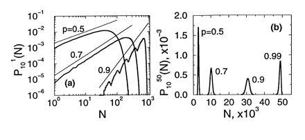
(a) The pdf of the number of molecules after n = 10 cycles and M₀ = 1 of a branching process with constant efficiency p, in log–log scale. Notice the multimodality for p = 0.9, and the power law regimes (straight lines). (b) Same as in a for M₀ = 50 (linear scale). The multimodality has disappeared even for p = 0.99.

To understand the features described above, it is convenient to use the formalism of generating functions (16). The generating function of P_n^M₀(N_n) is simply g_n,M0(s) = 〈s^N_n〉. Using Eq. 8, it is clear that g_1,1 = (1 − p)s + ps². It can be shown (17) that for a branching process

12

where we have denoted by g_1,1⁽ⁿ⁾(s) the nth composition of g_1,1(s) with itself, and used that g_0,M0(s) = s^M0 in the last equality. To proceed, we use the formalism of characteristic functions. The characteristic function φ_n,M0(ω) of the distribution of N_n having started with M₀ molecules, which is by definition the Fourier transform of P_n^M₀(N_n) (ref. 16), is simply φ_n,M0(ω) = g_n,M0(e^iω). In terms of the characteristic functions, Eq. 12 implies that

13

The characteristic function of the sum of M₀independent random variables is simply the product of the characteristic functions of each of them. Therefore, the physical interpretation of the last equation is that the amplification cascades produced by each of the M₀ original molecules proceed independently, without interaction. From this observation and the central limit theorem it follows that as the number of molecules M₀ becomes larger, the distribution of N_n tends to a Gaussian. This explains the observed features of the pdfs of Fig. 3b.

The behavior of the pdfs for finite M₀ in the limit of n → ∞ is a little bit more interesting. In fact, it is clear from Eq. 13 that it suffices to study the case M₀ = 1, which we do next. We should stress that our study of the asymptotically large n regime does not aim at understanding the behavior of PCR when infinitely many cycles are performed. In fact, we have shown in the previous section that the efficiency can be considered as constant only for a finite number of cycles. Rather, the reason for studying this asymptotic regime is that the convergence of the finite n case to the n → ∞ case is fast enough that many of the features arising for finite n are well explained by the study of asymptotically large n, most notably the power law behavior of the low N regime of Fig. 3a. It follows from Eq. 12 that g_n,1(s) = g_1,1[g_n−1,1(s)], which in terms of the characteristic functions and of the explicit expression for g_1,1(s) becomes

14

Given that we are going to consider the limit of n → ∞ and 〈N_n〉 = (1 + p)ⁿ (see Eq. 9) diverges in this limit, it is convenient to use the random variable Ñ_n = N_n/〈N_n〉. Denote by θ_n,1(ω) its characteristic function. It is easy to show that θ_n,1(ω) = φ_n,1(ω/(1 + p)ⁿ), which on using Eq. 14 yields

15

Notice that Eq. 15 can be thought of as a dynamical system, which maps the point z_n to z_n+1 ≡ f(z_n) = (1 − p)z_n + pz_n². The function θ_n,1(ω) (−∞ ≤ ω ≤ ∞) parametrizes a curve in the complex plane. In fact, the initial condition M₀ = 1 determines that θ_0,1(ω) = e^iω, which parametrizes the unit circle ζ₀. Subsequent applications of the map f(z) to ζ₀ produce the new curves ζ₁, ζ₂,…, which are parameterized respectively by θ_1,1(ω), θ_2,1(ω),…. The study of the limiting behavior of the pdf of Ñ_n is thus associated with the study of the invariant curves of the map f. Notice that the map f has only two fixed points, one at z = 0 (stable) and one at z = 1 (unstable). Upon iteration, all the infinitesimally small straight lines with slope λ passing through the repelling point z = 1 will generate a curve C_λ which is invariant under f, that is, f(C_λ) = C_λ. On the other hand, for any z ≠ 1 such that |z| ≤ 1, |f(z)| < |z|. Therefore the dynamics of this map brings all the points of ζ₀ (except for z = 1) to the origin. In the neighborhood of z = 1, ζ₀ is locally a straight line with slope λ = ∞, which upon evolution will become the invariant manifold C_∞. It follows that ζ_∞ coincides with C_∞, and θ_∞,1 parameterizes the invariant manifold of the map f, that crosses z = 1 parallel to the imaginary axis. Fig. 4a shows half the invariant manifold C_∞ corresponding to p = 0.9 (the other half is its complex conjugate), and on the same plot the imaginary part vs. the real part of θ_15,1(ω) (for positive ω). To the level of resolution of the figure no departures between the two curves are observed, meaning that the pdf of the number of molecules at 15 PCR cycles is well approximated by the limiting pdf.

Figure 4.

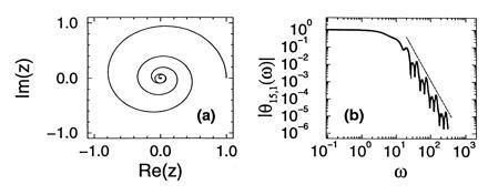
(a) The invariant manifold that crosses z = 1 tangent to the unit disk, of the map z_n+1 = (1 − p)z_n + pz_n² (with z in the complex plane), for p = 0.9. It is parametrized by θ_∞,1(ω). In the same plot the curve parametrized by θ_15,1(ω) is shown; it cannot be resolved from the invariant manifold. (b) Absolute value of θ_15,1(ω) (solid line) and the predicted power law (broken line).

This dynamical-system way of looking at the characteristic function of Ñ_n is very useful to understand the power law behavior of the pdfs of N_n. The argument goes as follows. Close to z = 0 (or equivalently, for large values of ω) the quadratic terms in Eq. 15 can be neglected, and the resulting approximate relation, θ_∞,1(ω) = (1 − p)θ_∞,1(ω/(1 + p)) accepts as a solution the ansatz θ_∞,1(ω) ≈ A(lnω)ω^{ln(1 − p)/ln(1 + p)}, where A(x) is in principle any periodic function with period ln(1 + p). The large ω behavior of the characteristic function θ_∞,1(ω) is then a power law, with logarithmically periodic modulations. That this is so is shown in Fig. 4b, where we have plotted the absolute value of θ_15,1(ω) for p = 0.9. The power law corresponding to the predicted scaling exponent of ln(1 − p)/ln(1 + p) is shown as the straight line close to the curve in the log–log plots of Fig. 4b. The implication of these results for the pdfs can be readily drawn. Recalling that the characteristic function and pdf are related through a Fourier transform, and that the Fourier transform of |ω|^α (with an appropriate infrared cutoff) scales as x^−α−1, we conclude that the pdf of Ñ_n should exhibit a scaling of the form P_∞¹(Ñ_n) ∼ Ñ_n^{[−ln(1 − p)/ln(1 + p) − 1]}. This scaling law is shown as the straight lines close to the curves plotted in log–log scale in Fig. 3a.

In the following section we use some of the results presented so far to analyze quantitative PCR.

Quantitative PCR

Although PCR is used mainly in a qualitative fashion, its potential for becoming an important tool in nucleic acid quantification in general (19), and in medical research in particular (20), has become clear in recent years. By quantitative PCR one means the use of the PCR to measure an unknown initial number of molecules M₀. A few techniques have been developed to that effect in the past, but the most widespread is probably the so-called competitive PCR (see, e.g., ref. 21). In this technique, the target, whose initial concentration is unknown, is amplified simultaneously with a standard, which is flanked by the same primers as the target and whose initial concentration is known. The standard should have a length different from that of the target, so that the two can be resolved in an electrophoretic gel. The basic idea in competitive PCR is that if the efficiencies of replication of the target and the standard are the same then the ratio of the concentration of target to that of the standard is constant in the reaction. Measuring that ratio at cycle n (where presumably we have enough concentration to use densitometric measurements) we can solve for the initial concentration of target. While this technique is very attractive, the basic assumption (the equality of the efficiencies in both species) has some drawbacks (22). Basically, the potential problems arise in the dependence of the efficiency on the length of the DNA molecule. The longer molecule will experience a decrease in efficiency before the shorter one does, as predicted in Eq. 7. In any case, the model presented here can be of use to assess the validity of the assumptions that go into the basics of competitive PCR.

In order for competitive PCR to work, the length of the standards has to be within a narrow window: it has to be sufficiently different from the length of the target molecules (to be resolved in a gel) and sufficiently similar to it in order for the equal efficiency assumption to work. The design of a good standard requires some ingenuity, and it has to be done on a case-by-case basis. In what follows we will present a design for measuring M₀ without the need of a standard. Suppose we measure the concentration of a given DNA molecule after a number of PCR cycles on a sample whose M₀ is unknown. One might think that if we repeated the same measurement for a reasonable number of times (say around 100 times, given that PCR equipment with capacity for 96 vials is not uncommon), so as to measure the mean value and the variance of the concentration across that number of experiments, we would have two equations (Eqs. 9 and 10) that can be solved for the two unknowns p and M₀. However, it can be shown that this procedure always yields two possible solutions for p and M₀, and there is no possible way, a priori, of choosing the right one. The reason for this is that for M₀ bigger than a few hundreds (which is nonetheless a small number of molecules), the distribution of N_n is Gaussian, and therefore determined only by the mean and the variance, which give the above-mentioned ambiguous answer.

Consider instead the following scheme. We prepare two sets of samples S₁ and S₂, each with K identical preparations and whose initial concentration of a given double-stranded DNA molecule is unknown. We run (under conditions for which p can be considered approximately constant from cycle to cycle) n₁ cycles of PCR on set S₁, and n₂ cycles on set S₂, after which we measure the number of molecules in every sample. The averages ν₁ and ν₂ over the K preparations in S₁ and S₂, are estimates of the ensemble averages μ_n1 and μ_n2 corresponding to Eq. 9 for n = n₁ and n = n₂, respectively. We can use that formula to compute m₀ = ν₁^{−n₂/(n₁ − n₂)} ν₂^{n₁/(n₁ − n₂)} as an estimate of the real M₀ and ρ = ν₁^{1/(n₁ − n₂)} ν₂^{−1/(n₁ − n₂)} − 1 as an estimate of the real p. Of course these estimates make sense only if a measure of the error involved in the method is provided. It takes a simple calculation to show that

16

and

17

18

In writing the last two equations we used Eq. 10. We tested these expressions in a set of very simple numerical simulations, whose details we are not going to report here except for saying that the PCR amplification was represented by the cascade given by Eq. 8. Under variations of all the parameters involved, Eqs. 16–18 were in excellent agreement with the numerical results. To get a flavor of the precision of the method proposed, assume a simple example with M₀ = 1000, p = 0.8, n₁ = 10, n₂ = 15, and K = 50. Under these conditions the above equations predict that the estimate of M₀ will be correct within 0.5% (that is, ±5 molecules) and that of p will be correct within 0.1%! These estimates refer to the purely statistical errors, and they will be fairly small under typical conditions. In real experiments they have to be supplemented with the errors involved in the measurement of the concentrations. If M₀ and p fluctuated from sample to sample (due to inevitable differences in their preparations), the fact that we are averaging over K samples will screen these fluctuations. In this latter case, Eqs. 16 will still be in agreement with the average M₀ and p, and Eqs. 17 and 18, which can be easily generalized to include these fluctuations, will give their right order of magnitude.

Summary

We have presented a kinetic model for the PCR, which can be the basis for a more accurate application of quantitative techniques, as it provides a dynamical account of the probability of replication as a function of the physical parameters involved. These include the rate constants of the different reactions. Conversely, the model allows us to extract information on these rates from direct measurements of p. From a theoretical point of view, it can also be used in the description of in vivo and in vitro enzymatic polymerization processes (23). The statistical analysis of PCR under the assumption of constant replication probability shows new interesting phenomena. The scaling behavior of the pdf is an effect of the recursivity of the process, whereas the multimodality is related to failures in replication during the first cycles. Although the latter is a phenomenon present only for a small number of initial molecules, it is not far from actual experimental conditions, and might be of relevance in quantitative applications.

Finally, we have used the statistical considerations of the fourth section to devise a method for measuring the initial number M₀ of molecules in a sample (quantitative PCR).

References

- 1.Mullis K B, Faloona F A. Methods Enzymol. 1987;155:335–350. doi: 10.1016/0076-6879(87)55023-6. [DOI] [PubMed] [Google Scholar]
- 2.Gibbs R A. Anal Chem. 1990;62:1202–1214. doi: 10.1021/ac00212a004. [DOI] [PubMed] [Google Scholar]
- 3.Gestland R, Atkins J, editors. The RNA World. Plainview, NY: Cold Spring Harbor Lab. Press; 1993. [Google Scholar]
- 4.Adleman L M. Science. 1994;266:1021–1024. doi: 10.1126/science.7973651. [DOI] [PubMed] [Google Scholar]
- 5.Kaplan P, Cecchi G, Libchaber A. In: Proceedings of the 2nd Annual Princeton Conference on DNA-Based Computation. Baum E, Boneh D, Kaplan P, Reif J, Seeman A, editors. Providence, RI: Am. Mathematical Soc.; 1996. in press. [Google Scholar]
- 6.Capson T L, Peliska J A, Kaboord B F, Frey M W, Lively C, Dahlberg M, Benkovic S J. Biochemistry. 1992;31:10984–10994. doi: 10.1021/bi00160a007. [DOI] [PubMed] [Google Scholar]
- 7.Patel S S, Wong I, Johnson K A. Biochemistry. 1991;30:511–525. doi: 10.1021/bi00216a029. [DOI] [PubMed] [Google Scholar]
- 8.Kuchta R D, Mizrahi V, Benkovic P A, Johnson K A, Benkovic S J. Biochemistry. 1987;26:8410–8417. doi: 10.1021/bi00399a057. [DOI] [PubMed] [Google Scholar]
- 9.Dahlberg M E, Benkovic J. Biochemistry. 1991;30:4835–4843. doi: 10.1021/bi00234a002. [DOI] [PubMed] [Google Scholar]
- 10.Kuchta R D, Mizrahi V, Benkovic P A, Johnson K A, Benkovic S J. Biochemistry. 1987;26:8410–8417. doi: 10.1021/bi00399a057. [DOI] [PubMed] [Google Scholar]
- 11.Sun F. J Comp Biol. 1995;2:63–86. doi: 10.1089/cmb.1995.2.63. [DOI] [PubMed] [Google Scholar]
- 12.Weiss G, von Haeseler A. J Comp Biol. 1995;2:49–61. doi: 10.1089/cmb.1995.2.49. [DOI] [PubMed] [Google Scholar]
- 13.Sambrook J, Fritsch E F, Maniatis T. Molecular Cloning: A Laboratory Manual. 2nd Ed. Plainview, NY: Cold Spring Harbor Lab. Press; 1989. [Google Scholar]
- 14.Yin H, Wang M D, Svoboda K, Landick R, Block S M, Gelles J. Science. 1995;270:1653–1657. doi: 10.1126/science.270.5242.1653. [DOI] [PubMed] [Google Scholar]
- 15.van Kampen N G. Stochastic Processes in Physics and Chemistry. Amsterdam: North-Holland; 1981. [Google Scholar]
- 16.Feller W. An Introduction to Probability Theory and Its Applications. 3rd Ed. I. New York: Wiley; 1968. [Google Scholar]
- 17.Harris T E. The Theory of Branching Processes. Berlin: Springer; 1963. [Google Scholar]
- 18.Athreya K B, Ney P E. Branching Processes. Berlin: Springer; 1972. [Google Scholar]
- 19.Ferre F. PCR Methods Applic. 1992;2:1–9. doi: 10.1101/gr.2.1.1. [DOI] [PubMed] [Google Scholar]
- 20.Clementi M, Menso S, Bagnarelli P, Manzin A, Valenza A, Varaldo P. PCR Methods Applic. 1993;2:191–196. doi: 10.1101/gr.2.3.191. [DOI] [PubMed] [Google Scholar]
- 21.Guilliland G, Perrin S, Blanchard K, Bumm F. Proc Natl Acad Sci USA. 1990;87:2725–2729. doi: 10.1073/pnas.87.7.2725. [DOI] [PMC free article] [PubMed] [Google Scholar]
- 22.Raeymaekers L. Anal Biochem. 1993;214:582–585. doi: 10.1006/abio.1993.1542. [DOI] [PubMed] [Google Scholar]
- 23.McAdams H H, Shapiro L. Science. 1995;269:650–656. doi: 10.1126/science.7624793. [DOI] [PubMed] [Google Scholar]