Bias and error in estimates of equilibrium free-energy differences from nonequilibrium measurements

Abstract

In 1997, Jarzynski proved a remarkable equality that allows one to compute the equilibrium free-energy difference ΔF between two states from the probability distribution of the nonequilibrium work W done on the system to switch between the states, e^–ΔF/kT = 〈e^–W/kT〉, [Jarzynski, C. (1997) Phys. Rev. Lett. 87, 2690–2693]. The Jarzynski equality provides a powerful free-energy difference estimator from a set of N irreversible experiments and is closely related to free-energy perturbation, a common computational technique for estimating free-energy differences. Despite the many applications of the Jarzynski estimator, its behavior is only poorly understood. In this article we derive the large N limit for the Jarzynski estimator bias, variance, and mean square error that is correct for arbitrary perturbations. We then analyze the properties of the Jarzynski estimator for all N when the probability distribution of work values is Gaussian, as occurs, for example, in the near-equilibrium regime. This allows us to quantitatively compare it to two other free-energy difference estimators: the mean work estimator and the fluctuation–dissipation theorem estimator. We show that, for near-equilibrium switching, the Jarzynski estimator is always superior to the mean work estimator and is even superior to the fluctuation–dissipation estimator for small N. The Jarzynski-estimator bias is shown to be the dominant source of error in many cases. Our expression for the bias is used to develop a bias-corrected Jarzynski free-energy difference estimator in the near-equilibrium regime.

Accurate measurement and calculation of free-energy differences is central to our understanding of biological, chemical, and physical molecular processes. A common method of estimating the free-energy difference ΔF = F_B – F_A between two states, A and B, of a classical system in contact with a heat reservoir is to perturb the system to induce a transition between these states. The average work done in such a perturbation satisfies 〈W〉 ≥ ΔF, where equality holds if and only if the perturbation is infinitely slow. An average of the work values obtained by any finite time experiment or simulation therefore overestimates the true ΔF. Until recently, recovering the equilibrium free energy from trajectories arbitrarily far from equilibrium was therefore thought to be impossible.

In 1997, however, Jarzynski (1, 2) proved an identity that relates the probability distribution of nonequilibrium work values with the equilibrium free-energy difference between the two states:

[1]

where β = (kT)^–1. On the left-hand side of this equation is an exponential of the equilibrium free-energy difference, and the right-hand side is an exponentially weighted average over an infinite number of nonequilibrium work trajectories, all started from the same initial equilibrium state. Although the second law of thermodynamics requires that the average work over all possible trajectories be greater than the free-energy difference, the work for an individual trajectory will occasionally be less (3). The Jarzynski average heavily weights these rare trajectories at the tail of the work distribution in order to recover ΔF. The Jarzynski equality is closely related to other recent advances in the theory of nonequilibrium statistical mechanics (4–7).

A recent single-molecule manipulation experiment verified the Jarzynski equality (8). A single folded RNA molecule was mechanically unfolded both reversibly and irreversibly, and the Jarzynski equality was used to obtain the free-energy change of the system (as estimated by the reversible work values) from the irreversible trajectories. This experiment was done at constant temperature and pressure, and therefore the Jarzynski equality was cast in terms of the Gibb's free energy ΔG rather than the Helmholtz free energy ΔF. A two-state model describing and justifying the outcome of these experiments was proposed recently (9). The Jarzynski equality can be applied at any point along the pulling trajectory, making it possible to reconstruct the entire free-energy profile of the molecule along the pulling coordinate (10).

The free-energy perturbation technique uses an identical averaging procedure to estimate free-energy differences but obtains the work values computationally (11–13). If a system is perturbed infinitely quickly from state A with Hamiltonian H_A to state B with Hamiltonian H_B such that its configuration, , remains unchanged, then the work that must be performed is . The Jarzynski relation is correct for arbitrary perturbation speeds, and thus we can recover the free-energy difference by averaging these work values over the equilibrium ensemble of configurations of state A (1):

This result was known long before the Jarzynski equality was proven, and we can view it as the Jarzynski equality in the limit of infinitely fast switching.

The Jarzynski equality therefore has many applications, but unfortunately the properties of the Jarzynski free-energy estimator

are largely unknown. How good is the Jarzynski estimator? If we sample from a given work distribution P(W) a total of N times (by unfolding an RNA molecule N times, for example), then how close will our final free-energy difference estimate be to the true ΔF? It is well known that the Jarzynski estimator is biased for finite N, meaning that the estimator has a systematic error. This bias can be the dominant source of error in estimating the free-energy difference, but the magnitude of the bias is generally unknown.

The Near-Equilibrium Regime and Free-Energy Difference Estimators

There are three common free-energy difference estimators that can be obtained from a set of N trajectories: the mean work estimator ΔF̂_MW, the fluctuation–dissipation (FD) theorem estimator ΔF̂_FD, and the Jarzynski estimator ΔF̂_J

[2]

〈...〉_N in these equations denotes an experimental average over N trajectories, and ΔF̂ represents an estimator of ΔF. The connection between these three estimators can be elucidated by writing Jarzynski's equality as a sum over the cumulants of the original work distribution (14):

[3]

The first four cumulants are

[4]

Note that the mean work estimator ΔF̂_MW is just an estimate of the first term on the right side of the cumulant expansion in Eq. 3 and is valid when the perturbation is done reversibly. The FD estimator ΔF̂_FD is simply an estimate of the first two terms of the cumulant expansion and is valid when the perturbation is done close to equilibrium.

The near-equilibrium regime is defined in this article as the regime in which the perturbation is sufficiently slow for the probability distribution of work P(W) to be Gaussian. It is important to note that, although being close to equilibrium requires a Gaussian work distribution, the inverse is not true. For example, a bead dragged through water by a Hookean spring has a Gaussian work distribution regardless of how fast the perturbation is done (15). The “near-equilibrium” results derived in this article therefore may be relevant even when the perturbation pulls the system far from equilibrium.

The near-equilibrium regime is important because the results are not model-dependent; any system perturbed slowly will have a Gaussian work distribution. In addition, the behavior of the Jarzynski estimator in this regime is a first-order estimate of the behavior in any regime. A Gaussian distribution has the unique property among probability distributions that only a finite number of its cumulants are nonzero. Specifically, only the first two cumulants are nonzero, and Eq. 3 shows that, in this regime, . The following important equality therefore holds in the near-equilibrium regime (16):

[5]

We have defined the dissipated work as the difference between the work and the equilibrium free-energy difference: W_dis = W – ΔF. Eq. 5 is one manifestation of the FD theorem (17) and suggests the particular expression given for the FD estimator in Eq. 2. In the near-equilibrium regime the variance of the work distribution yields, via the FD relation, an estimate of the dissipated work and hence of the expected overestimate inherent in the mean work estimator.

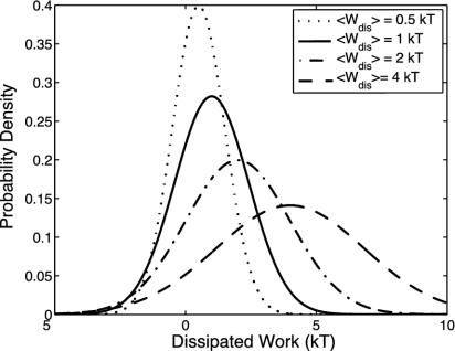
The Jarzynski equality can be expressed in terms of the dissipated work without reference to ΔF:1 = 〈e^–βWdis〉. In the near-equilibrium regime the probability distribution of dissipated work P(W_dis) is a Gaussian with mean W̄_dis and variance (see Eq. 5). Fig. 1 plots this Gaussian P(W_dis) for W̄_dis of 0.5, 1, 2, and 4 kT. As W̄_dis increases, the distribution becomes broader. The rare trajectories with negative dissipated work are those heavily weighted by the Jarzynski average, thus it is important to know how efficiently these trajectories are sampled. The probability of observing a trajectory with negative dissipated work is

This is a sharply decreasing function of W̄_dis, implying that the efficiency of sampling falls rapidly with increasing W̄_dis.

Fig. 1.

Gaussian probability distributions P(W_dis = W – ΔF) of dissipated work in the near-equilibrium regime for W̄_dis ≡ 〈W_dis〉 of 0.5, 1, 2, and 4 kT. As W̄_dis increases, the variance of the work distribution increases (), but P(W_dis < 0) decreases.

The Jarzynski equality states that e^–βΔF = 〈e^–βW〈 = ∫e^–βWP(W)dW, so the contribution to the estimate of a given part of the probability distribution is e^–βWP(W). In the case of Gaussian P(W), e^–βWP(W) is another Gaussian distribution with the same variance , but a mean given by (see Fig. 2). The most important part of the work distribution to sample therefore is the region

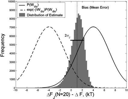
Fig. 2 plots, for the case of W̄_dis = 4 kT, the probability distribution of dissipated work P(W_dis) as well as the weighted probability distribution e^–βWdis P(W_dis).

Fig. 2.

Estimating ΔF from N = 20 near-equilibrium work values in the case of W̄_dis = 4 kT. The histogram plots ΔF̂_J(N = 20) –ΔF for 100,000 different estimates of ΔF, each obtained by a Jarzynski average of 20 work values sampled from a Gaussian work distribution (solid line). The dashed line corresponds to the contribution of the region to the average, e^–βWP(W). The dotted line is the bias (mean error): B_J(N = 20) = 〈ΔF̂_J (N = 20)〉 – ΔF ≈ 1.07 kT.

There are three important properties associated with any estimator of the free-energy difference:

[6]

The bias is simply the difference between the expectation value of the estimator and the true ΔF and therefore represents a systematic error. The expectation value of an estimator can be expressed by averaging over M free-energy estimates (each obtained from a set of N work values), and letting M → ∞:

[7]

The standard measure for the quality of an estimator is the MSE, which is a combination of the statistical error associated with σ²(N) and the systematic error associated with B(N). If the bias is zero, then 〈ΔF̂〉 = ΔF, and Eq. 6 shows that MSE(N) = σ²(N).

The Jarzynski estimator ΔF̂_J(N) = –β^–1 ln〈e^–βW〉_N is biased for all finite N as a result of the nonlinear averaging. By “biased” we mean that the difference 〈ΔF̂_J(N)〉 – ΔF ≡ B_J(N) is nonzero. This difference is caused by the imperfect sampling of the work distribution when only a finite number of trajectories are averaged. The presence of a bias is most obvious in the limiting case of a single trajectory being sampled (N = 1). In this case, the Jarzynski estimator is simply the work value measured because ΔF̂_J(N = 1) = –β^–1 ln e^–βW = W. The expectation value of the Jarzynski estimator in this case is therefore 〈ΔF̂_J(N = 1)〉 = 〈W〉 = ΔF + W̄_dis > ΔF, yielding a bias of B_J(N = 1) = W̄_dis.

Fig. 2 plots a histogram of ΔF̂_J(N = 20) – ΔF for near-equilibrium switching assuming W̄_dis= 4 kT. The dotted line is the bias, or mean error, of the Jarzynski estimator: B_J(N = 20) = 〈ΔF̂_J(N = 20)〉 – ΔF ≈ 1.07 kT. The variance of the estimator is the squared deviation about B_J (N = 20), whereas the MSE_J is the squared deviation about zero error (corresponding to the actual free-energy difference).

The Jarzynski Estimator in the Large N Limit

In this section we consider the behavior of the Jarzynski estimator in the large N limit for perturbations arbitrarily far from equilibrium. These results were derived independently by Zuckerman and Woolf (18). As shown previously, the Jarzynski bias B_J starts at B_J(N = 1) = W̄_dis. It then falls monotonically with increasing N (19) and approaches zero in the limit of infinite N. Assuming that the variance Var(e^–βW) is finite, the central limit theorem guarantees that, for sufficiently large N, the random variable Y = 〈e^–βW〉_N will be normally distributed with mean Ȳ = e^–βΔF and variance . We perform a linear expansion of ln (Y) around Y = Ȳ

[8]

This expression yields the bias for any well behaved [finite Var(e^–βWdis)] work distribution for N ≫ Var(e^–βWdis) or equivalently for B_J(N) ≪ kT.

To obtain the variance of the Jarzynski estimator (as defined in Eq. 6) in the limit of large N, we once again expand ln (Y) about Y = Ȳ and obtain

[9]

We see that, for large N and under very general conditions, there exists a simple relationship between the bias and variance of the Jarzynski estimator.

The MSE is simply a combination of the bias and variance of the estimator: . The large N limit is defined as N ≫ Var(e^–βWdis), so Eq. 9 gives . This implies that , making the variance the dominant source of noise in the large N limit.

Near-Equilibrium Regime

For the remainder of the article we focus on probability distributions of work that is Gaussian. This is always the case for perturbations done close to equilibrium but can also be true for perturbations far from equilibrium. If P(W) is Gaussian, then the mean 〈W〉 = ΔF + W̄_dis and variance have a simple relationship (Eq. 5).

Bias. Knowing the magnitude of the Jarzynski bias in the large N limit is useful, but in this limit, as shown above, the bias is not a significant source of error. In addition, we will show that the large N limit is often inaccessible by any experimental or computational strategy. More important therefore is the behavior of the bias for modest N, where the bias can be the dominant source of error for any technique using the Jarzynski estimator to recover a free-energy difference. Wood et al. (20) performed a linear expansion to prove that for small variance , the bias is . Unfortunately, this estimate is only valid for , excluding almost all situations of interest. For example, if W̄_dis = 5 kT, then at 50 sampled trajectories the above estimate yields a bias of only 0.1 kT, when in fact computational sampling from a Gaussian work distribution shows that the bias is ≈1 kT, i.e., 10 times larger. An improved estimate of the bias for larger W̄_dis and modest N is therefore highly desirable.

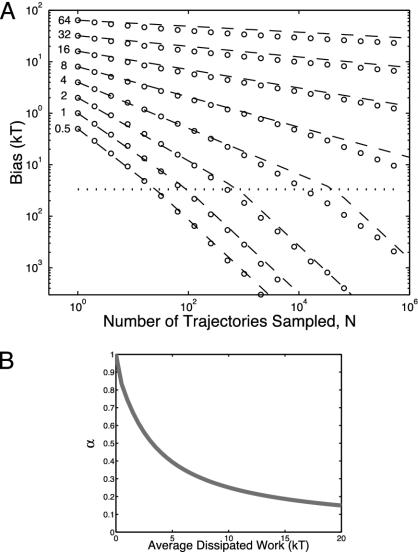
In the near-equilibrium regime, a log–log plot of the numerically calculated small N bias is approximately linear in N (see Fig. 3). This power law behavior of the bias at small N has been noted before and may be true even for systems perturbed far from equilibrium (21). We showed in The Near-Equilibrium Regime and Free-Energy Difference Estimators that B_J(N = 1) = W̄_dis, implying that for small N the bias can be approximated as

[10]

Systems with larger W̄_dis have a bias that falls off more slowly, meaning that α is a decreasing function of W̄_dis. To determine an accurate approximation for α(W̄_dis), we consider the limit of large N.

Fig. 3.

(A) Jarzynski bias as a function of N for average dissipated work of 0.5, 1, 2, 4, 8, 16, 32, and 64 kT. Each circle is the average of 150,000 sets of work values, each of size N (x axis). The dashed lines are the approximation derived in the text, with C = 15 (see Eqs. 10 and 11). The bias initially falls off as a power law B_J(N) = W̄_dis/N^α, with the fall-off rate α being a function of W̄_dis. The horizontal dotted line corresponds to the boundary between the small and large N regimes. (B) α as a function of W̄_dis. The bias falls off more slowly for larger W̄_dis.

In the near-equilibrium regime P(W) is Gaussian and our large N results (see Eq. 8) can be evaluated immediately:

[11]

As a consistency check, it is worth noting that, in the limit of small , our bias estimate reduces to the estimate of Wood et al. . For small , the large N limit occurs immediately, thus making the bias fall off as 1/N for all N. The first order term in our expansion of the bias has the form (e^2βW̄dis – 1)/N, which means that it is expected to be dominant if N ≫ (e^2βW̄dis – 1). We will therefore assume that the small N limit intersects the large N limit at N_C = C(e^2βW̄dis – 1):

[12]

C ≫ 1 is a constant that defines how small the bias must be before the large N limit is reached.

Fig. 3 plots B_J(N) for W̄_dis of 0.5, 1, 2, 4, 8, 16, 32, and 64 kT. The data points (circles) correspond to the numerically calculated bias averaged over 150,000 sets of N trajectories, and the dashed lines were obtained by assuming that the bias follows Eq. 10 in the small N regime and Eq. 11 in the large N regime (we have assumed C = 15). The single free parameter C defines the intersection point for the two regimes and completely specifies all eight curves. The fit is quite good, although for W̄_dis ≫ kT the bias initially falls more quickly than what would be predicted (see Eq. 13), leading to an average error of ≈20%. In addition, the computed bias smoothly interpolates between the two regimes at N ≈ N_C, thus falling below the crossing point of the estimated bias (especially for larger W̄_dis). Note that we used our analytic expression for the bias in the large N regime to determine the behavior of the bias for small N. This seems to work well despite the fact that the large N limit is often impossible to reach. For example, in the case of W̄_dis = 64 kT, the large N limit does not begin until N ≈ 10⁵⁷ work trajectories have been sampled. Most applications therefore fall in the small N regime.

Eq. 12 can be used to solve for α (W̄_dis), the rate at which the bias falls to zero in the small N regime:

[13]

Fig. 3B plots α as a function W̄_dis assuming that C = 15. We see that the bias falls off more slowly as W̄_dis increases, and that 1 ≥ α ≥ 0. The bias for small W̄_dis falls off approximately as 1/N, whereas W̄_dis = 5 kT yields, via Eq. 13, a value of α ≈ 0.4. It is important to be aware of the unexpectedly slow fall of the Jarzynski bias to avoid underestimating the bias and error in many applications (8, 22).

Variance. Once again it is helpful to consider the case of N = 1. The variance of the Jarzynski estimator then is simply the variance of the work distribution, . We therefore see that, in both the large N and N = 1 limits, (see Eq. 9), a relationship that does not hold at intermediate values of N. Nevertheless, for the regime W̄_dis ∼ kT, a procedure similar to that used for the bias yields the small N approximation,

[14]

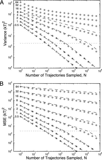
where the best fit is obtained with C_ν ≈ 50 in Eq. 13 determining α. The fact that C_ν > C means that the variance initially decays more quickly than the bias and hence that for small N. Fig. 4A plots for W̄_dis of 0.5, 1, 2, 4, 8, 16, 32, and 64 kT, with the small N approximation of Eq. 14 shown as a dashed line. For W̄_dis ≥ 5 kT, the variance cannot be approximated accurately by a power law and initially falls off faster than predicted by Eq. 13. The behavior of the variance for small N and large W̄_dis is therefore an area for future research, although in this regime the variance is not a significant source of error.

Fig. 4.

Variance (A) and MSE (B) of the Jarzynski estimator in the near-equilibrium regime for W̄_dis of 0.5, 1, 2, 4, 8, 16, 32, and 64 kT. Each point is the average of 150,000 sets of work values, each of size N (x axis). Dashed lines are the approximation derived in the text, with C_v = 50 for the variance curves and C_M = 40 for the MSE curves. The boundary between small and large N is denoted by the horizontal dotted line. The variance approximation in the small N regime is valid only for W̄_dis ∼ kT because, for W̄_dis ≫ kT, the small N variance does not follow power law behavior. In this regime the variance is not a significant source of noise.

MSE. The MSE_J(N) can be calculated by summing the variance of the estimator with the square of the bias. A summary of the properties of the Jarzynski estimator in the different regimes is available in Table 1. In most regimes the error is dominated by either the variance or bias of the Jarzynski estimator. Most applications are in the small N regime, where the bias is a significant (and often dominant) source of noise.

Table 1. Summary of the behavior of the Jarzynski estimator in the different regimes considered in this article.

	Arbitrary perturbation		Perturbations near equilibrium
	Small N	Large N	Small N		Large N
			W̄dis ∼ kT	W̄dis ≫ kT	All W̄dis
Bias, BJ(N)	?
Variance,	?			?
MSE	?

In the case of the bias we have α = In[2βCW̄_dis] /In[C(e^2βW̄_dis — 1) with C = 15, but for the variance α_V ≡ α (C = 50).

The most complicated situation is W̄_dis ∼ kT for small N, where both the variance and bias must be taken into account. In the near-equilibrium regime the MSE_J(N) is given by

[15]

For simplicity, we will assume for now that a single compromise value of C can be used to accurately describe the decay of both the variance and the bias B_J, making α_ν = α. In Fig. 4B we plotted MSE_J (N) for W̄_dis of 0.5, 1, 2, 4, 8, 16, 32, and 64 kT. The dashed line corresponds to Eq. 15 (assuming C_M = 40) in the small N regime and in the large N regime (Eq. 9). The expression for the variance used in Eq. 15 becomes invalid for W̄_dis ≫ kT, but in this regime the variance is not a significant source of error. Most of the overestimate of the error for W̄_dis ≫ kT is caused by the overestimate of the bias in Eq. 10.

We can invert Eq. 15 for the MSE_J (N) to get N (MSE_J), the number of trajectories that must be sampled to reach a given MSE:

[16]

It can be shown that this expression for the number of trajectories necessary to average over to obtain a given level of accuracy increases exponentially with W̄_dis. This means that Jarzynski averaging becomes unwieldy for large molecular systems and is experimentally impossible with macroscopic samples.

A common question in computational studies is whether a given amount of computer time should be used to perform a few slow runs (which therefore are close to equilibrium) or many fast runs (which therefore are further from equilibrium) (18). The expression for MSE_J (N) indicates that, as long as we are in the linear response regime (where W̄_dis is proportional to the perturbation rate and hence inversely proportional to the simulation time), a lower MSE is always obtained by performing fewer runs with smaller W̄_dis.

Comparing Three Free-Energy Difference Estimators

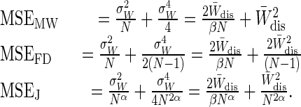
We are now able to compare the quality of the three free-energy estimators in the near-equilibrium regime(23):

[17]

These equations have several characteristics in common. The first term is proportional to W̄_dis and falls off as either 1/N or 1/N^α, whereas the second term is proportional to . The first term in the MSE_MW and MSE_FD equations is the error associated with estimating 〈W〉. The second term in the MSE_MW equation is the contribution of the bias, whereas the second term in the MSE_FD equation is the error inherent in estimating .

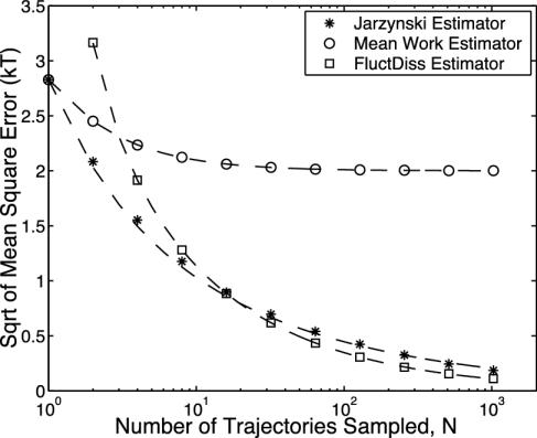
The square root of the three MSE functions is plotted as a function of N in Fig. 5 for the case of W̄_dis = 2 kT. The behavior of the MSE functions in this plot contains many general features. In the near-equilibrium regime, the Jarzynski estimator is always better than or equivalent to the mean work estimator. The errors are equal for N = 1, when the two estimators are identical, but the Jarzynski error then falls more quickly with increasing N. As W̄_dis → 0, the Jarzynski average is essentially a linear average similar to the mean work estimator, and the two estimators become identical. For larger values of W̄_dis, the Jarzynski estimator quickly becomes superior to the mean work estimator. For example, at the relatively small dissipation of W̄_dis = 4 kT, we already have that . This means that, for W̄_dis ≥ 4 kT, it is better to do a Jarzynski average of two work values than to take the mean of an infinite number of work values. A simple conclusion of this analysis is that the Jarzynski estimator is always better than the mean work estimator for near-equilibrium switching.

Fig. 5.

Plot of the square root of the MSE for each of the three different estimators in the case of near-equilibrium switching and W̄_dis = 2 kT. Each point is the result of numerical calculation, and the dotted line is the theoretically predicted error (Eq. 17). Note that the Jarzynski estimator is best for N ≤ 16 despite the fact that we are considering the near-equilibrium regime where the FD estimator is unbiased. The Jarzynski estimator is always superior to the mean work estimator.

The Jarzynski estimator is also superior to the unbiased FD estimator for small N. This is perhaps surprising because we are considering the near-equilibrium regime, where the FD estimator is unbiased. The FD estimator works poorly for small N because of the inherent difficulty of estimating from limited data. For larger N the FD estimator is better than the Jarzynski estimator in the near-equilibrium regime. For arbitrary perturbations the Jarzynski estimator is expected to be superior to the FD estimator for all N, because the FD estimator will become biased.

Bias Correction

In this section we show that understanding the behavior of the bias allows us to construct an improved Jarzynski free-energy difference estimator. The most obvious bias correction is to use as an estimate for the dissipated work, thus yielding as an estimate bias and making of the the final estimator

[18]

This improves the estimator, but is an underestimate of W̄_dis (because of the Jarzynski bias), and thus the bias correction will generally be too small.

A first-order correction is therefore to use , resulting in a final free-energy difference estimator of

[19]

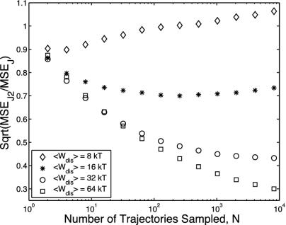
The effect of using the bias-corrected estimator ΔF̂_J1 in the nearequilibrium regime for W̄_dis of 8, 16, 32, and 64 kT is shown in Fig. 6. Bias correction decreases the typical errors (), especially equilibrium regime for W̄_dis. The error improvement deteriorates for small W̄_dis and large N, because the bias becomes overcorrected. In this regime ΔF̂_J1 has a lower error. Bias correction for W̄_dis ∼ kT must be done by using more sophisticated methods such as incorporating a technique called block averaging with the bias correction presented above [typical decreases in error are 20% (unpublished results)].

Fig. 6.

Ratio of to for average dissipated work of 8, 16, 32, and 64 kT (see Eq. 19). This form of bias correction is more effective for large W̄_dis, partly because the bias is overcorrected for small W̄_dis and large N. Correcting for the bias in the case of W̄_dis ∼ kT requires more complicated techniques.

Conclusions

Although Jarzynski averaging is an important and widespread technique for calculating free-energy differences, the behavior of the estimator is poorly understood. In particular, the most common method for estimating error is simply to examine the statistical error among repeated experiments. This technique can fail dramatically in the many situations where the bias is the dominant source of error. In addition, a substantial amount of effort must be invested before it can be determined whether a given strategy is practical. This article provides a quantitative estimate for the number of work trajectories that must be sampled to achieve a given MSE as a function of the average dissipated work.

The comparison between the three free-energy estimators in the near-equilibrium regime also leads to several concrete conclusions. First, the mean work estimator should never be used, even for very large systems with concomitantly large dissipated work. The Jarzynski estimator is expected to be optimal for systems that are perturbed violently. Less expected, however, is that the Jarzynski estimator should also be used in the near-equilibrium regime when insufficient data are available to accurately estimate the variance (which is necessary to use the FD estimator). This is often the case because the near-equilibrium regime is only accessed by perturbing the system slowly, thus requiring a large amount of computation.

A better understanding of the behavior of the Jarzynski estimator will allow researchers to develop improved sampling and averaging algorithms. As a preliminary step in that direction, we have shown that a quantitative understanding of the behavior of the Jarzynski estimator bias in the near-equilibrium regime makes it possible to improve the estimator by correcting for the bias.

An obvious direction for future research is to determine how well the methods presented here can be used to analyze the small N behavior of the Jarzynski bias and variance for perturbations arbitrarily far from equilibrium. Another important area of study is the behavior of the Jarzynski estimator when the work is measured in the presence of noise. The experimental realities of single-molecule techniques imply that measurement noise will often be an appreciable fraction of the desired signal.

References

- 1.Jarzynski, C. (1997) Phys. Rev. Lett. 78 2690–2693. [Google Scholar]
- 2.Jarzynski, C. (1997) Phys. Rev. E Stat. Phys. Plasmas Fluids Relat. Interdiscip. Top. 56 5018–5035. [Google Scholar]
- 3.Wang, G. M., Sevick, E. M., Mittag, E., Searles, D. J. & Evans, D. J. (2002) Phys. Rev. Lett. 89 050601. [DOI] [PubMed] [Google Scholar]
- 4.Crooks, G. E. (2000) Phys. Rev. E Stat. Phys. Plasmas Fluids Relat. Interdiscip. Top. 61 2361–2366. [Google Scholar]
- 5.Yamada, T. & Kawasaki, K. (1967) Prog. Theor. Phys. 38 1031. [Google Scholar]
- 6.Evans, D. J., Cohen, E. G. D. & Morriss, G. P. (1993) Phys. Rev. Lett. 71 2401–2404. [DOI] [PubMed] [Google Scholar]
- 7.Gallavotti, G. & Cohen, E. G. D. (1995) Phys. Rev. Lett. 74 2694–2697. [DOI] [PubMed] [Google Scholar]
- 8.Liphardt, J., Dumont, S., Smith, S., Tinoco, I., Jr., & Bustamante, C. (2002) Science 296 1832–1835. [DOI] [PubMed] [Google Scholar]
- 9.Ritort, F., Bustamante, C. & Tinoco, I., Jr. (2002) Proc. Natl. Acad. Sci. USA 99 13544–13548. [DOI] [PMC free article] [PubMed] [Google Scholar]
- 10.Hummer, G. & Szabo, A. (2001) Proc. Natl. Acad. Sci. USA 98 3658–3661. [DOI] [PMC free article] [PubMed] [Google Scholar]
- 11.Beveridge, D. & DiCapua, F. (1989) Annu. Rev. Biophys. Biophys. Chem. 18 431–492. [DOI] [PubMed] [Google Scholar]
- 12.McCammon, J. A. (1991) Curr. Opin. Struct. Biol. 1 196–200. [Google Scholar]
- 13.Frenkel, D. & B. Smit, (1996) in Understanding Molecular Simulation: From Algorithms to Applications (Academic, San Diego).
- 14.Zwanzig, R. (1954) J. Chem. Phys. 22 1420–1426. [Google Scholar]
- 15.Mazonka, O. & Jarzynski, C. (1999) arXiv:cond-mat/9912121.
- 16.Hermans, J. (1991) J. Phys. Chem. 95 9029–9032. [Google Scholar]
- 17.Callen, H. B. & Welton, T. A. (1951) Phys. Rev. 83 34–40. [Google Scholar]
- 18.Zuckerman, D. & Woolf, T. (2002) Phys. Rev. Lett. 89 180602. [DOI] [PubMed] [Google Scholar]
- 19.Zuckerman, D. & Woolf, T. (2002) arXiv:, cond-mat/0208015.
- 20.Wood, R. H., Muhlbauer, W. C. F. & Thompson, P. T. (1991) J. Phys. Chem. 95 6670–6675. [Google Scholar]
- 21.Zuckerman, D. & Woolf, T. (2002) Chem. Phys. Lett. 351 445–453. [Google Scholar]
- 22.Hendrix, D. & Jarzynski, C. (2001) J. Chem. Phys. 114 5974–5981. [Google Scholar]
- 23.Hummer, G. J. (2001) J. Chem. Phys. 114 7330–7337. [Google Scholar]