Magnetic Field Shift due to Mechanical Vibration in Functional Magnetic Resonance Imaging

Abstract

Mechanical vibrations of the gradient coil system during readout in echo-planar imaging (EPI) can increase the temperature of the gradient system, and alter the magnetic field distribution during functional magnetic resonance imaging (fMRI). This effect is enhanced by resonant modes of vibrations and results in apparent motion along the phase encoding direction in fMRI studies. The magnetic field drift was quantified during EPI, by monitoring the resonance frequency interleaved with the EPI acquisition, and a novel method is proposed to correct the apparent motion. The knowledge on the frequency drift over time was used to correct the phase of the k-space EPI dataset. Since the resonance frequency changes very slowly over time, two measurements of the resonance frequency, immediately before and after the EPI acquisition, are sufficient to remove the field drift effects from fMRI time series. The frequency drift correction method was tested “in vivo” and compared to the standard image realignment method. The proposed method efficiently corrects spurious motion due to magnetic field drifts during fMRI.

INTRODUCTION

Growing demands on MRI systems to speed up image acquisition have led to the use of higher magnetic fields and to the development of ultra fast imaging techniques, e.g., echo planar imaging (EPI). Rapidly switched gradient fields during EPI-readout interact with the static magnetic field producing strong time dependent mechanical forces in the gradient coil system that can stimulate natural modes of vibration in the coil assembly(1), and produce large vibrational amplitudes in on-resonance conditions(2).

Friction between vibrating parts of the MRI scanner transforms mechanical vibration energy into heat thereby increasing their temperature. Ferromagnetic shim elements frequently are attached to the vibrating gradient coil; therefore vibrations can transiently increase their temperature and reduce their magnetization, which ultimately changes the homogeneity and strength of the local magnetic field. Even slight magnetic field shifts during EPI can lead to large apparent movements of the object in the phase encoding direction in fMRI studies(3-6). If not corrected properly, such mismatches of the object's position in subsequent images may result in erroneous activation patterns in fMRI analyses(7,8).

In this work we propose a simple approach to monitor the water resonance frequency during EPI experiments with interleaved one-dimension free-induction-decay (1D-FID) acquisitions, which provide high-resolution spectral information. We show that the frequency drift caused by vibration related thermal effects, as observed in our system, is sufficiently slow in time; therefore the instant frequency can be determined by using two measures of the resonance frequency: immediately before and after the EPI timeseries, and linear interpolation in between. We demonstrate that these measurements can be used to correct the observed frequency drift during EPI experiments by linear phase correction of the EPI k-space data. This approach does not significantly increase the overall scan time, effectively corrects apparent motion artifacts and minimizes spurious activation in fMRI analyses; it can be easily combined with other retrospective methods (9-13) to further correct for real motion in fMRI studies.

METHODS

Data acquisition

All studies were performed on a 4-Tesla MRI scanner driven by a Varian INOVA console. The self-shielded whole-body SONATA-Siemens gradient system is connected to three K2217 Siemens Cascade Gradient Power Amplifiers (peak voltage and current: 2000 V, and 500 A, respectively) that produce gradient pulses up to 44 mT/m peak amplitude with a 0.25 msec minimum rise time. The mechanical vibrations of the gradient coil were measured with piezoelectric transducers (PZT; Radio Shack, 273−073A), using 500 μsec 22 mT/m rectangular gradient pulses, as reported earlier(2).

Two different EPI protocols were used: a) with a readout gradient repetition rate (1/2δt) of 1220 Hz (219 kHz receiver bandwidth), matching the main resonance mode of vibration of the gradient coil assembly, and, b) mismatching this resonance mode using a gradient repetition rate of 1160 Hz (200 kHz receiver bandwidth). The former protocol will be referred to as “Loud”, and the latter as “Quiet”. Figure 1 shows the time course of the first readout cycles for both protocols, and Fig. 2 illustrates the locations of these frequencies and the gradient coil system's vibrational response(2), using a logarithmic scale. Note that only minimal timing changes in the EPI experiment result in a four-fold difference in vibrational amplitude.

Figure 1.

Time course of the first readout z-gradient cycles for “Loud” (solid line) and “Quiet” (dotted line) EPI-protocols. EPI-Readout frequencies: 1220 Hz (“Loud”) and, 1160 Hz (“Quiet”).

Figure 2.

Frequency response curve showing the amplitude of vibrations as a function of the EPI-readout z-gradient frequency. Fine adjustment (< 10%) of the acquisition bandwidth resulted in a four-fold (12 dB) increase of the vibration amplitude from “Quiet” to “Loud” EPI protocols.

Both protocols were used to image a static 15cm-diameter spherical water-phantom (30 coronal slices, 4 mm slice thickness, 1 mm gap, 48×64 matrix size, 4.1×3.1 mm in-plane resolution, TE/TR = 25/3000ms, 2400 time points, 2 hours). The water resonance frequency was measured at each time point by using a simple one-dimension free-induction-decay (1D-FID) experiment immediately after EPI acquisition. Subsequently, the recovery of the system was monitored over a ten-hour period with FID acquisitions only, using TR = 6000 ms. In order to guarantee identical initial conditions the scanner was left inactive for at least twelve hours before experiments.

Data analysis

EPI images were reconstructed in IDL (RSI Research Systems Inc., Boulder CO) using a Hamming filter and a phase correction method that produced minimal ghost artifacts(14). The 1D FID data was eight-fold zero filled to 24k, whereby the original digital resolution of 1/3 Hz (3072 complex data points, 2048 Hz spectral width) was interpolated to 0.04 Hz. The extensive use of interpolation increased the accuracy of the full width half maximum (FWHM) measurements. This approach is more robust and time efficient for the analysis of large numbers of time points compared to Lorentzian fits of automatically phased real-part spectra. The instantaneous resonance frequency and linewidth were determined by the maximum absolute value of the water peak and its FWHM, respectively. The frequency drift over time, Δω_o(t), was fitted to a bi-exponential function:

$$\Delta {\omega }_0\left(\mathit{t}\right)={\mathit{A}}_0+{\mathit{A}}_1{\mathit{e}}^{-(t-t_0)∕{\tau }_1}+{\mathit{A}}_2{\mathit{e}}^{-(t-t_0)∕{\tau }_2},$$ [1]

where A₀, A₁, A₂, τ₁, τ₂ are the fitting parameters, and t₀ is a time offset constant that was set to zero for the exponential growth fits (during EPI acquisitions), and to 120min for the bi-exponential decay fits (during the following recovery without EPI acquisition).

The value of the frequency drift during the EPI acquisition (Eq. 1) was used to correct the apparent motion artifact in each individual image by calculating a linear phase correction:

$${\alpha }_m\left(\mathrm{t}\right)=m\cdot \Delta {\omega }_{\mathrm{o}}\left(\mathrm{t}\right)\cdot \delta \mathrm{t},$$ [2]

where the phase encoding step, m, is an integer that may be positive or negative depending on its position in the acquisition matrix and δt is the interval between two consecutive phase encoding blips, as indicated in figure 1. The corrected k-space data S^corr(t) was obtained from the acquired data S(t) by

$${\mathit{S}}^{corr}\left(\mathit{t}\right)=\mathit{S}\left(\mathit{t}\right){\mathit{e}}^{-i{\alpha }_m\left(t\right)}.$$ [3]

The validity of this correction was demonstrated by realignment of the phase corrected and uncorrected images with the statistical parametric mapping package SPM2 (Welcome Department of Cognitive Neurology, London UK) (16), using a six rigid-body transformation. The images also were spatially smoothed with SPM2, using a 8mm Gaussian kernel.

In vivo acquisition

With the participation of a healthy volunteer (39 year-old female), we demonstrated the feasibility of the proposed method in vivo. Written consent was obtained prior to the study, which was approved by the Institutional Review Board at Brookhaven National Laboratory.

An EPI-timeseries with 160 time points was acquired using the EPI-FID “Loud” protocol as defined above in the absence of any particular stimulation. Apparent motion during image acquisition was determined for corrected and uncorrected datasets. Additionally, a set of T1-weighted anatomical images was obtained with the FLASH (15) technique (TE/TR = 10/700ms, 1.5 × 1.5 × 5.0 mm³ spatial resolution, 28 sagital slices, matrix size = 128 × 128).

Statistical analysis

A voxel-by-voxel statistical analysis was applied to the data, using a general linear model and block designs, to identify spuriously activated and deactivated brain areas. Four different models were tested: an asymmetric activation model with four blocks [20 time points “ON”; 20 time points “OFF”] a) with, and b) without high-pass (HP) temporal filtering [128 seconds cut-off period], c) a symmetric design with additional “OFF” periods (10 time points) at the beginning and end of the block design (four “ON” blocks; three “OFF” blocks) and HP filtering, and, d) a symmetric design with eight blocks (10 time points “ON” ; 10 time points “OFF”) and HP filtering. We employed the four statistical models (asymmetric, HP-asymmetric, HP-symmetric, and HP-high-frequency-symmetric) to derive activation maps for the uncorrected dataset before and after realignment in SPM2, as well as for the frequency drift corrected dataset (non-realigned). Activation patterns were overlaid on subject's T1-structure. Clusters with at least 10 voxels (500 mm³) were considered significant in the statistical analysis of brain activation, using a voxel-level threshold p = 0.005.

RESULTS

The experiments in phantom demonstrated the drift of the resonance frequency (Fig 3) during EPI-acquisition (120 min; 2400 timepoints) and during the subsequent recovery periods (600 min; 6000 timepoints). During EPI, the resonant frequency increased steadily and peaked at the end of the EPI acquisition period (0 − 120 min); for the “Loud” protocol the maximum frequency drift was about five times larger than that for the “Quiet” protocol. After the ten-hour recovery, the frequency offset returned to its initial value as measured before the start of the EPI acquisition period.

Figure 3.

Resonance frequency drift during EPI acquisition [1−120min, gray block] with “Loud” (black solid line) and “Quiet” (dark gray solid line) protocols, and the subsequent recovery time without EPI acquisition [white block].

Figure 4 shows the linewidth of the water resonance peak as a function of time. There was a small but noticeable line broadening (ΔFWHM ≅ 0.008ppm, and 0.020ppm for “Quiet”, and “Loud” scans) during the EPI acquisitions that exponentially returns to its initial value during the recovery period. The increased linewidth (and noise) during the two-hour EPI-acquisition period possibly originates from time-dependent changes associated to dynamic fluctuations of the magnetic field distribution as reported by Wu et al.(16), or remaining eddy current effects. As an example, Fig 4 also shows the 1D-FID spectra for the “Loud” and “Quiet” protocols, at t = 2.5 min, and at the end of the recovery period (for the “Quiet” protocol only), demonstrating the asymmetric line broadening effect.

Figure 4.

Linewidth changes during EPI acquisition [1−120min, gray block] for “Loud” (black solid line) and “Quiet” (dark gray solid line) protocols, and the subsequent 10-hours of recovery without EPI acquisition [white block] (only first 4 hours shown). Sample spectra for both protocols are given during the EPI acquisition period (a, b) and at the end of the recovery period (c) of the “Quiet” acquisition (results for “Loud” are similar at this time point).

The exponential fitting results are summarized in Table1. The duration of the EPI acquisition period proved to be insufficient to assure good fitting stability for the bi-exponential fitting model during this period. To assess a potential bi-exponential field growth the EPI acquisition should be prolonged (∼ ten hours); however, the safety limits of our scanner's hardware restrict continuous acquisitions to less than two hours. Therefore, only mono-exponential fitting was used during the EPI-periods, yielding time constants of 101±1 min, and 77±1 min for the “Loud” and “Quiet” protocols, respectively. In contrast, bi-exponential fitting was used during the long recovery periods and resulted in a short time constant of approximately 40min, for both “Loud” and “Quiet” protocols, and long time constants of 141±1 min, and 171±1 min for the “Loud”, and “Quiet” protocols, respectively. The quality of the linewidth dataset also permitted mono-exponential fitting only; time constants of 18±1 min, and 11±1 min were found for the “Loud” and “Quiet” protocols, respectively.

Table 1.

Fitting Parameters for increasing (0−120min) and decreasing (120−720min) resonance frequency shift Δω (Fig 3), and linewidth (FWHM; Fig.4) for “Loud” and “Quiet” protocols, respectively.

fitting function: f(t) = A0 + A1e−(t−t0)/τ1 + A2e−(t−t0)/τ2
curve	t [min]	t0 [min]	A0	τ1 [min]	A1	τ2 [min]	A2	chi2
Δωloud	0−120	0	179.8±0.1	n/a	n/a	77±1	−172.4±0.1	0.008
Δωloud	120−720	120	−1.72±0.01	40±1	43.7±2	141±1	99.5±0.2	0.053
FWHMloud	120−720	120	7.5±0.1	11±1	2.6±0.1	n/a	n/a	0.01
Δωquiet	0−120	0	52.4±0.04	n/a	n/a	101±1	−52.5±0.04	0.002
Δωquiet	120−720	120	−0.23±0.01	41±1	4.3±0.2	117±1	33.1±0.2	0.014
FWHMquiet	120−720	120	7.5±0.1	18±1	1.2±0.1	n/a	n/a	0.04

The resonance frequency drift (Fig. 3) produced an apparent displacement of the object (phantom) during the EPI experiment that was quantified by image realignment in SPM (Fig. 5 original datasets). Alternatively, we employed the measured frequency to correct the time series for translations along the phase encoding direction; the remaining spurious displacement was quantified by image realignment (Fig 5, corrected datasets). The frequency drift based correction can correct up to 98% (a ten-fold reduction) of the spurious motion, demonstrating the effectiveness of the method. The quality of the correction is similar for the “Loud” and “Quiet” protocols, showing only small translation differences (< ±0.2 mm) that fall within the error-range of the realignment algorithm.

Figure 5.

Apparent translation along the phase encoding direction in EPI images for “Loud” (black, and gray solid lines correspond to the original, and corrected datasets, respectively) and “Quiet” (dashed, and dotted lines correspond to the original, and corrected datasets, respectively) acquisition protocols. The 2400 time points were realigned in SPM2. Maximum translations = 11.6 mm and 3.2 mm, for “Loud” and “Quiet”, respectively.

Figure 6 shows the resonance frequency during an 8 min “in vivo” EPI acquisition demonstrating the approximately linear behavior of the frequency drift during the relatively short experiments under real imaging conditions. As indicated by the dotted line, we subsequently used only the initial and final frequency offsets and a linear interpolation in between for the corrections; small non-linear effects were ignored, for being hardly above the limit of precision for the method. Figure 7 depicts the translation in the phase encoding direction, before and after correction; translations in the other two remaining directions were both below 0.2 mm and the three rotations angles were less than 0.5 degrees for both corrected and uncorrected images (data not shown).

Figure 6.

Resonance frequency drift (solid line) during in vivo EPI (“Quiet” protocol) and linear interpolation (dotted line) between endpoints.

Figure 7.

Apparent translation, quantified by SPM2-image realignment, for in vivo EPI images (“Quiet” protocol): original dataset (solid) and corrected (dotted).

Figure 8 illustrates the findings of the activation analysis for all motion-correction methods (rows: uncorrected, frequency drift corrected, and realigned) and statistical analyses (columns: asymmetric, asymmetric with high-pass filter, symmetric with high-pass filter, and high-frequency symmetric with high-pass filter). Positive correlations (p < 0.005) with statistical models are shown in red; negative correlations (deactivations) are blue. For the unfiltered asymmetric design, the large clusters of spurious activation at the surface of the head are due to uncorrected apparent motion (Fig 8a); twelve large clusters (corrected for multiple comparisons) of spurious activation are significant (p_corrected<0.05), in the whole brain. The use of a HP filter (Fig 8b), and a symmetric statistical model (Fig 8c) reduced spurious activation. The high-frequency symmetric model (Fig 8d) minimizes the spurious activation; only three significant clusters remain significant in the whole brain. Both, the frequency-drift correction method (without motion correction; Figs 8e-h), and the retrospective motion-correction (Figs 8i-m) reduce the spurious activation to levels comparable to the uncorrected high-frequency symmetric model (Fig 8d).

Figure 8.

Residual motion-related spurious activation for uncorrected (top – a, b, c, d), realigned (middle – e, f, g, h), and frequency drift corrected time series (bottom – i, k, l, m), using four different statistical (block design) models: asymmetric without HP (left – a, e, i), and with HP filter (center-left – b, f, k), symmetric with HP filter (center-right – c, g, l), and high-frequency symmetric with HP filter (right – d, h, m). Spurious activation (red), or deactivation (blue) clusters with at least 10 voxels (500 mm³) were considered significant, using a threshold p < 0.005. Experiment was based on the “Quiet” protocol. Cut-off frequency of the HP filter = 1/128 Hz. Activation patterns were overlaid on structural images reconstructed from a sagital FLASH acquisition.

DISCUSSION

During EPI, apparent translation along the phase encoding direction resulted from a drift in resonance frequency (Fig. 3). Image displacement increases during EPI acquisition, and decreases subsequently, both in an exponential manner. The process is slow suggesting a thermal origin. Image sets obtained with two different EPI-readout frequencies were compared: one in resonance with the principal mode of vibration of the gradient coil system, the second off-resonance. The large difference in frequency drift, and the consequent apparent object dislocation can only be explained by a thermal process that involves mechanical vibration, since the two protocols were otherwise almost identical (see figure 1). The small alteration of the gradient amplitude and duty cycle does not engender a sufficient difference in power deposition to account for the observed heating effect. The slight variation in the gradient timing is equally unlikely to produce any significant difference in eddy currents that could explain the observed phenomenon. The actively shielded design of the gradient coil set used in this study also supports the argument that eddy currents do not contribute substantially to the observed phenomenon. Therefore, we suggest a process in which friction, between the ferromagnetic shim elements and the shimming slot insert, transforms the vibration energy into heat, increasing the temperature and reducing the magnetization of the shim elements, thereby changing the scanner's magnetic field.

The analysis of the linewidth (Fig. 4) indicates the presence of dynamic line broadening effects during the EPI acquisition, which might be due to residual eddy currents, but more likely are the result of the vibration of the assembly itself producing an acoustic-magnetic coupling as reported by Wu et al.(16). A second thermal mechanism might be responsible for the faster recovery of the linewidth after EPI acquisition, compared to that of the frequency shift; this effect is small in comparison to the large drift of the static magnetic field and does not produce visible image artifacts. This second order effect is probably related to thermal dilatation of the coil assembly, thereby slightly changing the position of the passive shim elements, and consequently introducing small high-order alterations in the magnetic field.

Two different heat-transfer processes can explain the bi-exponential behavior of the frequency shift during recovery: Specifically, we suggest that the two different time constants result from heat conduction between A) the ferromagnetic shim elements and the whole coil assembly (slow heat-exchange pathway), and, B) the coil system and the water-cooling circuit (fast heat-exchange pathway). In this model, the water-cooling system is a thermal reservoir with (approximately) constant temperature; it is also strongly coupled to the coil assembly, which has a far larger heat capacitance than the small shim elements. During EPI acquisition additional processes have to be considered: The suggested friction-induced heating of C) the shim elements, and, D) other vibrating parts of the coil assembly, and finally, E) the Joule transformation of electric energy to heat in the resistive copper wires. Figure 9 illustrates the complete model.

Figure 9.

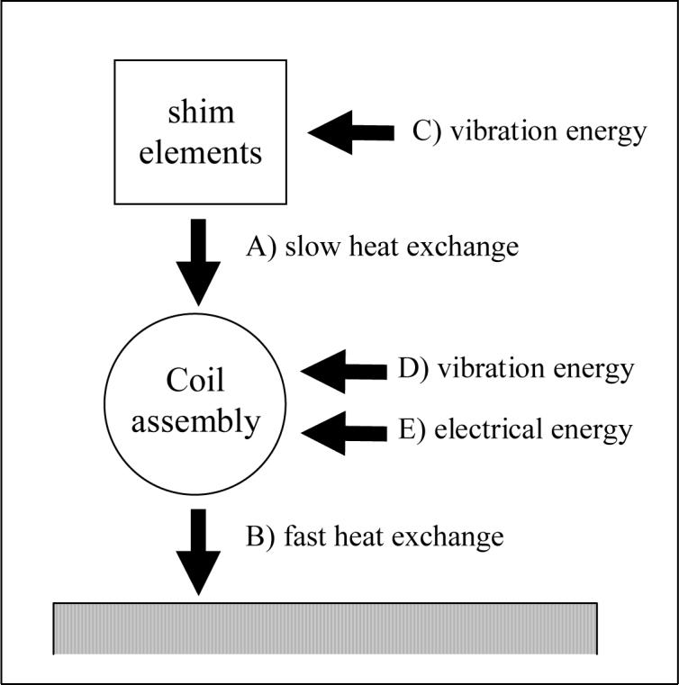
Schematic heat transfer model. Heat exchange pathways A and B between the shim elements, coil assembly, and the water cooling system are responsible for bi-exponential temperature decay during system recovery. Two energy sources contribute during EPI acquisition: C) vibration directly increases the temperature in the shim elements and, D) the coil assembly including vibrating parts other than the shim elements. Finally, E) electrical currents in the coils also increase the temperature of the coil assembly.

For the mono-exponential field-increase during EPI acquisitions, we found that the time constant, which results from both the “slow” and “fast” thermal pathways, is longer for the “Quiet” protocol, compared to the “Loud” protocol. This suggests that for the lower energy deposition during “Quiet” scans, the “slow” thermal pathway has a relatively higher contribution. During “Loud” scans, the high-energy deposition caused by vibration of the whole coil assembly might overload the water-cooling pathway. For the bi-exponential field-recovery without EPI acquisition, we recorded the same short time constant for “Quiet” and “Loud” protocols, demonstrating the same “fast” pathway with time constant, τ₁ ≅ 40 min. The long time constant (τ₂) was smaller for the “Quiet” compared to the “Loud” protocol; however, its relative amplitude (A₂/A₁) was higher for the former. This finding also suggests that the “slow” thermal pathway is slightly dominant when the vibration is less intense (“Quiet” scans). Lastly, the longer mono-exponential recovery of the linewidth (FWHM) during “Quiet” scans also supports the dominance of the “slow” pathway for the “Quiet” scans. To gain more insight about the involved thermal processes it would be desirable to simplify the possible thermal pathways by switching off the water-cooling system; unfortunately, hardware limitations did not allow this in the present study.

The zero-order magnetic field change (frequency drift) introduces large apparent motion artifacts in the time series over a 2 hour EPI acquisition (Fig. 5: 8mm for “Loud”, and 2 mm for “Quiet” scans), in agreement with previous studies(17). We demonstrated that this artifact can be reduced to a small remaining displacement of less than 0.2 mm, by applying a time-domain linear phase correction based on measurements of the frequency drift. The remaining apparent displacement represents the sensitivity limit of the method due to noise in the frequency offset acquisition, curve fitting errors, and statistical noise in the realignment process used to quantify the displacement.

The in vivo study demonstrates that the observed frequency drift varies slowly enough over time to be linearly approximated. Therefore, the frequency drift can be corrected with only two measurements of the resonant frequency: immediately before and after the acquisition of the time series. The activation maps demonstrate that the frequency drift correction successfully suppresses spurious activation due to apparent motion (Fig. 8).

Slowly varying frequency drifts have been reported repeatedly(17-22). The resulting apparent motion artifacts(3-6) can be corrected either by directly removing the frequency drift as demonstrated here or by standard image realignment(9-13). However, realignment algorithms can eventually introduce spurious activation even in the absence of real object motion(23,24). Although this is not generally considered to be a serious problem we would like to alert about the possibility, especially when using low frequency stimulation models. The prior removal of frequency drifts, as described here, can potentially turn the common retrospective for real object motion more robust, thereby avoiding possible spurious activation in fMRI. Compared to corrections derived from phase measurements(19,25), our approach has superior sensitivity (< 10⁻³ ppm/time point) in detecting frequency drifts and other sufficiently slow instabilities.

CONCLUSION

Apparent motion artifacts along the phase encoding direction can emerge in fMRI time series as a result of magnetic field drifts. Intense vibrations of the gradient coil assembly during EPI can lead to friction-induced heating of ferromagnetic shim elements, thereby transiently reducing their magnetization and changing the homogeneity and strength of the local magnetic field. Since stimulation of resonant vibration modes of the gradient coil system can greatly increase vibration amplitudes, correct imaging parameters should be chosen to avoid these resonant modes. In this work, we monitored the magnetic field drift during, and after the acquisition of EPI time series. The field increases exponentially during EPI acquisition, and exponentially returns to baseline afterwards. The shift is slow compared to the length of typical EPI time series. For short time series (∼10 minutes in our system), a phase correction method based on a linear interpolation between two measures of the resonant frequency (immediately before and after the EPI acquisition) efficiently corrects the spurious translation along the phase encoding direction. For longer time series, intermediate frequency measurements might be necessary. This simple method can potentially increase accuracy of image realignment algorithms, and minimize spurious motion artifacts.

REFERENCES

- 1.Hedeen RA, Edelstein WA. Characterization and prediction of gradient acoustic noise in MR imagers. Magn Reson Med. 1997;37:7–10. doi: 10.1002/mrm.1910370103. [DOI] [PubMed] [Google Scholar]
- 2.Tomasi D, Ernst T. Echo Planar Imaging at 4Tesla with Minimum Acoustic Noise. J Magn Reson Imaging. 2003;18:128–130. doi: 10.1002/jmri.10326. [DOI] [PubMed] [Google Scholar]
- 3.Duerk JL, Simonetti OP. Theoretical aspects of motion sensitivity and compensation in echo-planar imaging. J Magn Reson Imaging. 1991;1(6):643–650. doi: 10.1002/jmri.1880010605. [DOI] [PubMed] [Google Scholar]
- 4.Slavin GS, Riederer SJ. Gradient moment smoothing: a new flow compensation technique for multi-shot echo-planar imaging. Magn Reson Med. 1997;38(3):368–377. doi: 10.1002/mrm.1910380304. [DOI] [PubMed] [Google Scholar]
- 5.Jaffer FA, Wen H, Jezzard P, Balaban RS, Wolff SD. Centric ordering is superior to gradient moment nulling for motion artifact reduction in EPI. J Magn Reson Imaging. 1997;7(6):1122–1131. doi: 10.1002/jmri.1880070627. [DOI] [PubMed] [Google Scholar]
- 6.Jezzard P, Clare S. Sources of distortion in functional MRI data. Hum Brain Mapp. 1999;8:80–85. doi: 10.1002/(SICI)1097-0193(1999)8:2/3<80::AID-HBM2>3.0.CO;2-C. [DOI] [PMC free article] [PubMed] [Google Scholar]
- 7.Hajnal JV, Myers R, Oatridge A, Schwieso JE, Young IR, Bydder GM. Artifacts due to stimulus correlated motion in functional imaging of the brain. Magn Reson Med. 1994;31(3):283–291. doi: 10.1002/mrm.1910310307. [DOI] [PubMed] [Google Scholar]
- 8.Friston KJ, Williams S, Howard R, Frackowiak RS, Turner R. Movement-related effects in fMRI time-series. Magn Reson Med. 1996;35(3):346–355. doi: 10.1002/mrm.1910350312. [DOI] [PubMed] [Google Scholar]
- 9.Cox RW. AFNI: Software for analysis and visualization of functional magnetic resonance neuroimages. Comput Biomed Res. 1996;29:162–173. doi: 10.1006/cbmr.1996.0014. [DOI] [PubMed] [Google Scholar]
- 10.Woods R, Grafton S, Holmes C, Cherry S, Mazziotta J. Automated image registration: I. General methods and intrasubject, intramodality validation. J Comput Assist Tomogr. 1998;22(1):139–152. doi: 10.1097/00004728-199801000-00027. [DOI] [PubMed] [Google Scholar]
- 11.Friston KJ, Ashburner J, Frith CD, Poline JB, Heather JD, Frackowiak RSJ. Spatial registration and normalization of images. Hum Brain Mapp. 1995;2:165–189. [Google Scholar]
- 12.Jenkinson M, Smith S. A global optimisation method for robust affine registration of brain images. Med Image Anal. 2001;5(2):143–156. doi: 10.1016/s1361-8415(01)00036-6. [DOI] [PubMed] [Google Scholar]
- 13.Gold S, Christian B, Arndt S, Zeien G, Cizadlo T, Johnson DL, Flaum M, Andreasen NC. Functional MRI statistical software packages: A comparative analysis. Hum Brain Mapp. 1998;6:73–84. doi: 10.1002/(SICI)1097-0193(1998)6:2<73::AID-HBM1>3.0.CO;2-H. [DOI] [PMC free article] [PubMed] [Google Scholar]
- 14.Buonocore MH, Gao L. Ghost artifact reduction for echo plannar imaging using image phase correction. Magn Reson Med. 1997;38:89–100. doi: 10.1002/mrm.1910380114. [DOI] [PubMed] [Google Scholar]
- 15.Haase A, Frahm J, Hanicke W, Merboldt KD. FLASH imaging. Rapid NMR imaging using low flip angle pulses. J Magn Reson. 1986;67:257–266. doi: 10.1016/j.jmr.2011.09.021. [DOI] [PubMed] [Google Scholar]
- 16.Wu Y, Chronik BA, Bowen C, Mechefske CK, Rutt BK. Gradient-induced acoustic and magnetic field fluctuations in a 4T whole-body MR imager. Magn Reson Med. 2000;44:532–536. doi: 10.1002/1522-2594(200010)44:4<532::aid-mrm6>3.0.co;2-q. [DOI] [PubMed] [Google Scholar]
- 17.Kochunov P, Liu H, Andrews T, Gao J, Fox P, Lancaster J. A B0 Shift Correction Method Based on Edge RMS Reduction for EPI fMRI. J Magn Reson Imag. 2000;12:956–959. doi: 10.1002/1522-2586(200012)12:6<956::aid-jmri21>3.0.co;2-5. [DOI] [PubMed] [Google Scholar]
- 18.Sutton B, Noll D, Fessler J. Dynamic Field Map Estimation Using a Spiral-In/Spiral-Out Acquisition. Magn Reson Med. 2004;51:1194–1204. doi: 10.1002/mrm.20079. [DOI] [PubMed] [Google Scholar]
- 19.Durand E, Van de Moortele P, Clouard M, Bihan D. Artifact Due to B0 Fluctuations in fMRI: Correction Using the k-Space Central Line. Magn Reson Med. 2001;46:198–201. doi: 10.1002/mrm.1177. [DOI] [PubMed] [Google Scholar]
- 20.Ward H, Riederer S, Jack C., Jr Real-Time Autoshimming for Echo Planar Timecourse Imaging. Magn Reson Med. 2002;48:771–780. doi: 10.1002/mrm.10259. [DOI] [PubMed] [Google Scholar]
- 21.Van de Moortele P, Pfeuffer J, Glover G, Ugurbil K, Hu X. Respiration-Induced B0 Fluctuations and Their Spatial Distribution in the Human Brain at 7 Tesla. Magn Reson Med. 2002;47:888–895. doi: 10.1002/mrm.10145. [DOI] [PubMed] [Google Scholar]
- 22.Henry P, Van de Moortele P, Giacomini E, Nauerth A, G B. Field-Frequency Locked In Vivo Proton MRS on a Whole-Body Spectrometer. Magn Reson Med. 1999;42:636–642. doi: 10.1002/(sici)1522-2594(199910)42:4<636::aid-mrm4>3.0.co;2-i. [DOI] [PubMed] [Google Scholar]
- 23.Freire L, Mangin J. Motion Correction Algorithms May Create Spurious Brain Activations in the Absence of Subject Motion. Neuroimage. 2001;14:709–722. doi: 10.1006/nimg.2001.0869. [DOI] [PubMed] [Google Scholar]
- 24.Thacker NA, Burton E, Lacey AJ, Jackson A. The effects of motion on parametric fMRI analysis techniques. Physiol Meas. 1999;20(3):251–263. doi: 10.1088/0967-3334/20/3/303. [DOI] [PubMed] [Google Scholar]
- 25.Thesen S, Krüger G, Müller E. Absolute correction of B0 fluctuations in echo-planar imaging. Vol. 11. Proc. Intl. Soc. Mag. Reson. Med.; Toronto, Canada: 2003. p. 1025. [Google Scholar]