Computational Resources for Cryo-Electron Tomography in Bsoft

Abstract

The Bsoft package (Heymann and Belnap JSB 2007, 157, 3) has been enhanced by adding utilities for processing electron tomographic (ET) data; in particular, cryo-ET data characterized by low contrast and high noise. To handle the high computational load efficiently, a workflow was developed, based on the database-like parameter handling in Bsoft, aimed at minimizing user interaction and facilitating automation. To the same end, scripting elements distribute the processing among multiple processors on the same or different computers. The resolution of a tomogram depends on the precision of projection alignment, which is usually based on pinpointing fiducial markers (electron-dense gold particles). Alignment requires accurate specification of the tilt axis, and our protocol includes a procedure for determining it to adequate accuracy. Refinement of projection alignment provides information that allows assessment of its precision, as well as projection quality control. We implemented a reciprocal space algorithm that affords an alternative to back-projection or real space algorithms for calculating tomograms Resources are also included that allow resolution assessment by cross-validation (NLOO2D); denoising and interpretation; and the extraction, mutual alignment, and averaging of tomographic subvolumes.

1. Introduction

Cryo-electron tomography is opening new vistas in molecular and cellular structural biology (Baumeister and Steven, 2000; Subramaniam and Milne, 2004). The requirements for producing optimal tomograms are firstly the quality of the tilt series of micrographs, and secondly the computational processing of these data. In ongoing efforts to enhance our tomographic capabilities, which hitherto have been applied primarily to pleiomorphic and asymmetric virus particles and other protein complexes (Grunewald et al., 2003; Harris et al., 2006; Heymann et al., 2006), we continue to develop relevant computational resources.

Here we describe the implementation of tomography-specific utilities in the software package, Bsoft (Heymann, 2001; Heymann and Belnap, 2007). The primary aim is to provide the user with tools to perform the projection alignment and reconstruction in an efficient manner. A secondary aim is to make processing as easy as possible for the user, without losing control of the important parameters and still allowing detailed manipulation. Underlying both aims is a capability to handle, in the form of a database, the large number of parameters generated in a tomographic analysis. In Bsoft, this is accomplished through the use of parameter files. For some operations, e.g. micrograph alignment and reconstruction, we developed new code; for others, we simply incorporated pre-existing programs into Bsoft, making them readily accessible in a processing framework in which a user may seamlessly access the other image processing operations currently supported. While some of the same functionality is available in other packages, such as IMOD (Kremer et al., 1996), TOM (Nickell et al., 2005) and EM3D (Ress et al., 1999), we attempted to provide a clear workflow associated with a parameter database and adhering to the 3DEM conventions (Heymann et al., 2005).

2. Materials and Methods

2.1 Tilt series acquisition

To illustrate and analyze the various processing steps for tomography, tilt series of vitrified specimens of coated vesicles (Heymann and Belnap, 2007; Heymann et al., 2006) and herpes simplex virus type 1 (HSV-1) A-capsids (Cardone et al., 2007) were used. In brief, a Tecnai-12 electron microscope (FEI, Hillsboro, OR) operating at 120 keV and equipped with an energy filter (Gatan, Inc.) was used to record single-axis tilt series at 1° steps, covering ranges of ~ −70° to +70°, at a defocus of ~4 µm with a cumulative dose of ~ 60 electrons/Ų. Data were recorded under low-dose conditions, using SerialEM (Mastronarde, 2005).

2.2 Aligning the tilt series

We implemented a procedure for aligning tilt series based on the well known method of using gold fiducial markers. The tilt series is first preprocessed by normalizing the images with bnorm and generating the first parameter file with btomo or bshow. To prepare for the alignment, parameters such as the pixel size, the tilt axis angle and the tilt angles are set, and a marker seed is picked in bshow. If the tilt axis angle is not well known for the microscope and the magnification used, it needs to be determined more accurately by running a set of single iterations of btrack with tilt axis angles close to the expected value. This is then followed by a multi-iteration tracking of the markers through the tilt series by building a 3D marker model and determining the origins of the individual micrographs, using the nominal tilt axis angle and tilt angles. The result can be inspected in bshow and errand markers manually corrected. Finally, a full geometric refinement of the micrograph views, origins and scales, and the 3D marker model is done with btrack. (See Supplementary Material for more detail)

2.3 Reconstruction

The tomograms are reconstructed in reciprocal space using oversampling and a nearest neighbor algorithm, using btomrec. The fiducial markers used in the tilt series alignment can be removed (“painted” by replacement with the image average) from the micrographs before reconstruction. (See Supplementary Material for more details).

2.4 Determining resolution

The quality of the tomogram may be assessed by the noise-compensated leave-one-out (NLOO) method of Cardone et al. (Cardone et al., 2005). Because of the inherent anisotropy of the reconstruction, the resolution is assessed in 2D for each micrograph in the series. The NLOO approach involves the calculation of the ratio of two Fourier ring correlation (FRC) curves, the first a comparing each micrograph with an appropriate reprojection of a tomogram without that micrograph, and the second comparing the micrograph with a reprojection of the full tomogram. In the original implementation based on weighted backprojection, in addition to the full tomogram, another tomogram needed to be calculated for every micrograph. Here we make use of the central section theorem, also known as the Fourier slice theorem (Kak and Slaney, 1988), to simplify and accelerate the calculation, requiring only the reconstruction of two 2D central sections for comparison to each micrograph. Because the beam is not perpendicular to all but one of the micrographs, the corresponding voxels between two Fourier transforms is offset perpendicular to the tilt axis as a function of the tilt angles. This is included in calculating the central sections in addition to the basic geometric transformations (see Appendix).

Resolution is assessed with btomres, which calculates the resolution for one micrograph at a time based on the refined alignment of the tilt series. This is then repeated for every micrograph in the series, providing a trivial basis for concurrent computation. Because the Fourier transforms of the micrographs are required for calculating the resolution for each one, they can be initially generated with bmgft. With this approach the computational cost for estimating the resolution for the whole tilt series is comparable to that needed to generate a single reconstruction. The resolution estimation can be accelerated by using only a limited subset of micrographs with tilt angles close to that for the central section being reconstructed. A C-shell script, tomres, is available for calculating the resolution for a complete tilt series and for distributed processing.

2.5 Extraction and analysis of subtomograms

Often features of interest occupy only limited portions of a tomogram. In these cases the reconstructed volume can be visually inspected in bshow, and sub-regions containing these features manually marked, in the same way as already available for 2D particles. Selected sub-volumes are then extracted from bshow or with bpick for further processing. If several copies of a feature are contained in a tomogram, they can be extracted with this approach, then oriented with respect to a reference using the program bfind, which does a brute force angular search with shifts obtained from 3D cross-correlation with the option to compensate for the missing wedge. Once the particle maps are oriented, they can be added with badd to generate an average map with improved signal-to-noise ratio.

As another option for the analysis of a localized feature, the coordinates of the regions marked in the tomogram can be used to extract sub-tilt series from the original series using bsubvol. These series contain only fields of view corresponding to the projection from the selected volumes and exclude other unwanted regions. As shown in the Results, the local resolution analysis is one possible application of interest for the extraction of sub-tilt series. The resolution is estimated in the same way as for the full micrographs, but restricted to a selected feature or subregion. This could form the basis of local alignment to improve the quality of sub-volume reconstructions, as demonstrated within other contexts (Cantele et al., 2007; Iwasaki et al., 2005).

2.6 Denoising by filtering or averaging

Three types of denoising filters have been implemented in Bsoft: (i) bmedian does iterative median filtering (van der Heide et al.), (ii) bbif does bilaterial filtering (Jiang et al., 2003), and (iii) bnad does non-linear anisotropic diffusion filtering (Frangakis and Hegerl, 2001, Fernandez et al. 2003). A particle with symmetry can be rotated to a standard orientation by comparison with a reference map with the program bfind, and symmetrized to average out noise with bsym. Alternatively, the location of symmetry axes can be determined with bsym to establish the orientation, followed by symmetrization.

2.7 Workflow

The workflow for tomographic analyses in Bsoft focuses on the transfer of parametric information between programs. The general layout followed for processing is as given by Heymann and Belnap (Heymann and Belnap, 2007) (Figure 1). The parameter file may be viewed as a database that is modified and grows as the processing progresses. The first parameter file generated may only contain references to the tilt series with the appropriate nominal tilt parameters. Selecting a marker seed in bshow adds the marker records to the zero-degree projection data block. The result of btrack contains the marker records for all the micrographs. When a reconstruction is calculated, a data block is added with the appropriate parameters, such as its file name and voxel size. When particles (subtomograms) are picked from the tomogram, appropriate records are appended to the reconstruction data block. The final parameter file therefore contains all of the parameters accumulated, as well as a history of the commands used. This record allows the user to also go back to an earlier parameter file and run the programs with different processing parameters.

Figure 1.

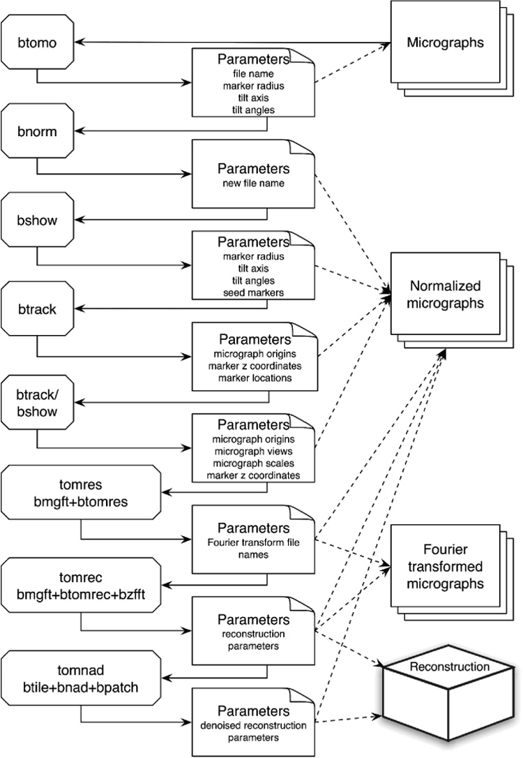
Workflow of tomographic processing in Bsoft, showing the programs on the left, the parameter files in the middle and the actual images on the right. Solid lines indicate direct I/O, while dashed lines indicate references to the image files. In the parameter file boxes, the parameters changed at that stage are listed. The last three boxes on the left refer to scripts that can be run across a distributed processing system.

3. Results and Discussion

3.1 Tilt series alignment

3.1.1 Micrograph normalization

Processing of a tilt series starts with normalizing the micrographs. The biggest variation in the signal recorded with constant exposure per micrograph is its decrease at higher tilt because the path length of the beam through the specimen increases. This is equivalent to an increase in specimen thickness of 1/cos(α) with the tilt angle α. The decrease in beam intensity as a function of the tilt angle is therefore:

$$I(\alpha )=I_o{e}^{-\frac{t_o}{\Lambda \text{cos}(\alpha +\Delta \alpha )}}$$ (1)

where I_o is the incident beam intensity, t_o is the specimen thickness at zero-tilt, and Λ is the mean free path. The addition to the tilt angle, Δα, accounts for the specimen being already tilted with respect to the specimen holder and perpendicular to the tilt axis, e.g., in cases where the microscope grid might be bent or the carbon layer is not completely planar and may sag within a grid square. We examined the micrograph averages of the tilt series taken with the same dose for each image as a measure of the signal strength. Figure 2A shows one such curve and illustrates that the signal intensity may be described, to a reasonable approximation, by equation 1 with a mean free path of 1600 Å at 120 kV (Feja and Aebi, 1999). The thickness, t_o, was estimated a posteriori by inspection of the reconstructed tomogram and compared to the calculated thickness (Figure 2B). The agreement is imperfect because other factors may be involved. For instance, the use of equation 1 in this manner has the inherent assumption that the specimen is homogenous between individual micrographs and even between tilt series. Nevertheless, this experiment illustrates the relationship between signal attenuation and tilt angle. The normalization of the tilt series is therefore based on the micrograph averages. The middle part of the histogram of each micrograph is fitted to a Gaussian curve, and the average and standard deviation adjusted to user-defined values.

Figure 2.

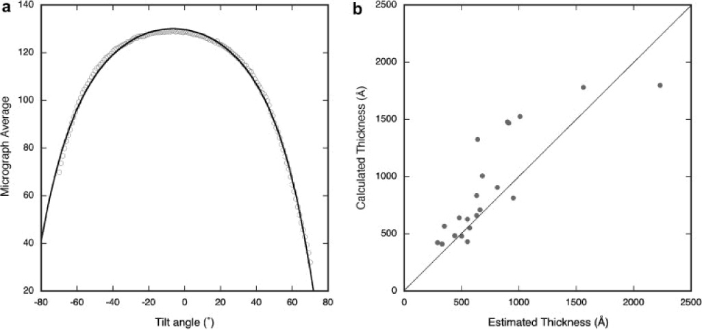
(A) Variation of the micrograph average is a function of the thickness or path length of the electron beam passing through the specimen. The asymmetry of the curve can be partially attributed to the tilt of the specimen volume with respect to the plane perpendicular to the electron beam. The fitted curve corresponds to: $I=203e^{\frac{710\AA }{1600\AA \text{cos}(\alpha +6.5\mathrm{Ϸ})}}$ where the thickness of the center of the tomogram was estimated at ~ 660 Å by inspection of the reconstructed tomogram. (B) The specimen thickness estimated by inspection of the reconstruction compared to that calculated from the micrograph averages.

3.1.2 Determination of the tilt axis angle

Projection alignment is sensitive to the initial choice of the tilt axis angle. The first iteration of alignment gives an average residual (an estimate of the overall marker location error) that is good enough to assess the accuracy of the tilt axis angle. Doing this with a range of angles around the expected tilt axis angle can be used to find it more accurately (Figure 3). While this is a somewhat time-consuming process, it may be expedited by distribution over a cluster of processors. Once the tilt axis angle is known for a particular tilt series, it should remain very similar for other tilt series taken with the same microscope and at the same magnification.

Figure 3.

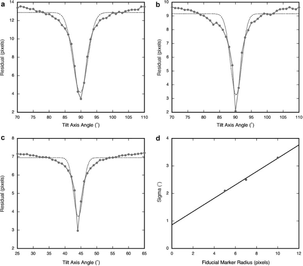
The tilt axis angle is determined by running one iteration of tracking with a range of tilt axis angles, and choosing the angle giving the smallest residual. The fiducial marker radii for tilt series taken at different magnifications were (A) 10 pixels (54500x), (B) 7 pixels (38500x), and (C) 5 pixels (26000x). The width of the inverse peak expressed as the sigma coefficient of a Gaussian curve fitted to the profile (broken lines in A–C), is a function of the marker radius (D), determining how accurately the tilt axis angle must be specified for successful tracking.

Alignment is also sensitive to the size of the fiducial markers. We determined the residual error for tilt axis angle ranges for three tilt series taken at three different magnifications (Figure 3A–C). The effort to find the z-coordinate of each marker during tracking is confined to the vicinity of a line perpendicular to the tilt axis. If there is a sizable error in the tilt axis angle, the resulting determination of the z-coordinates will be poor or completely wrong. In Figure 3D, the relationship between the size of the fiducial marker and the width of the inverted peak of the tilt axis angle search is shown. From these tests it is clear that with a large fiducial marker image (radius of 10 pixels or more), the tilt axis angle must be known to within 2°, while for smaller markers (radius of 5 pixels or less), it must be known to within 1° or better. In general the size of the fiducial marker should be chosen so as to have a radius of at least 7 pixels in the projections.

3.1.3 Tilt series alignment

In the zero degree tilt micrograph, a set of seed markers is picked manually or automatically by cross-correlation with a synthetic marker reference. The tracking is then done from the low to high tilt angles, progressively improving the z-coordinates of the 3D marker model while at the same time determining the translational alignment of each projection. This process is repeated until the changes in marker positions are small enough (less than one pixel on average), or until a user-set limit on the number of iterations is reached. In the majority of tilt series that we have analyzed that had well determined tilt-axis angles, only the minimum of two iterations were needed (2 in 15 required more than 2 iterations).

The trajectories of the markers corrected for the projection shifts may be examined for sudden deviations that would indicate poorly located markers or markers that moved (Figure 4A). Deviation of the trajectories from linearity may also indicate that the tilt axis is not be exactly perpendicular to the beam. A direct estimate of the departure from perpendicularity, called the “level” angle, may be obtained during the course of projection alignment. In our microscope the level angles are very small, indicating that the stage is well aligned.

Figure 4.

Postscript output from tracking fiducial markers. (A) Trajectories of the markers perpendicular to the tilt axis to show individual marker deviations and possible rotation of the tilt axis out of the xy plane. (B) Marker errors enlarged ten-fold to reveal badly positioned markers. The tilt axis is shown as a dashed line.

Differences observed between the indicated marker positions in the projections, and their predicted positions from the 3D marker model, may reflect errors in assigned marker positions, or marker movement. Figure 4B shows an exaggeration of these errors, giving the impression of random movement of the markers within a limited region. Visual inspection of the marker positioning (i.e., whether the circles in bshow correspond well to the evident markers) suggests that their placement is accurate to within a pixel or two, which certainly may contribute significantly to an average error of 1–2 pixels. This does not rule out the possibility of marker movement, but places a limit on it of 1–2 pixels (~5–20 Å, depending on the magnification). We did not observe any trends in marker movement, indicating that any such movement is highly restricted and random.

3.1.4 Scale refinement

Attempts to refine scaling in the x and y directions yielded deviations from one of about 0.001, with a maximum of about 0.004 at the high tilts. In reciprocal space and considering the resolution achieved, this translates into a fraction of a reciprocal space voxel during reconstruction. This is not considered to have a significant effect on the quality of tomograms for vitrified specimens (although distortions in plastic sections may require scaling corrections). Efforts to iteratively refine scaling yielded increased compensation for tilting (i.e., the scaling perpendicular to the tilt axis deviated more and more from one, while the scaling parallel to the tilt axis remained close to one). It is therefore risky to introduce scaling early in the orientation refinement, and it is recommended to only refine scaling once at the end, if needed.

3.1.5 Comparisons with other software packages

One of the key features of the alignment described here, is that it is based on the gradual construction of a 3D marker model during the tracking stage. Finding the markers with btrack is successful in the majority of cases, with problems usually arising with the highest tilt images where the marker contrast falls off severely and interactive correction is required. In IMOD (Kremer et al., 1996), marker tracking is done between successive micrographs and typically leads to many omissions and errors that need to be fixed by hand. In EM3D (Ress et al., 1999), markers are selected in all micrographs and the correspondence of markers between micrographs determined afterwards.

Once the marker locations in the micrograph is known, the refinement of the 3D marker model and the micrograph view geometry is a non-linear problem that can be solved in many ways. We chose to provide options to refine parts of the problem (such as the z-coordinates of the 3D marker model, and the micrograph shifts and orientations) for robustness and speed, and to allow the user to select a refinement strategy. This can be done completely automatically and in our experience yielded excellent solutions. Fewer refinement parameters are exposed compared to IMOD (Kremer et al., 1996), where the user can select to couple various parameters to increase robustness. More complex algorithms have been devised to solve the refinement problem (Brandt and Ziese, 2006; Lawrence et al., 2006), but we do not see the fundamental advantage of having a more elaborate solver.

We did comparisons of the alignment results on the same data sets between the programs described here and those from IMOD (Kremer et al., 1996). We restricted the alignment parameters in IMOD to resemble those used with btrack (excluding distortions, magnification or scale changes, and in-plane rotations), and obtained very similar marker residuals. The main difference was that the marker tracking with btrack was fully automatic with minor manual adjustments afterwards, while the tracking in IMOD required significant interactive remediation. We conclude that our approach of marker model-based tracking provides a more efficient way of finding the marker locations. In addition, with our examples, we did not find it necessary to correct for distortions and scale changes, because the marker residuals covered much smaller length scales than the expected resolution. In addition, our approach allows us to refine an independent geometric view for each micrograph, thus inherently compensating for an issue such as the tilt axis not being perfectly perpendicular to the electron beam (as dealt with in (Diez et al., 2006); we understand that this issue is not resolved in IMOD yet).

3.2 Reciprocal space reconstruction

The most commonly used method used for tomographic reconstruction is weighted back-projection (Radermacher et al., 1986) as for example, in IMOD (Kremer et al., 1996)). There has also been some use of the iterative real-space methods, ART (Marabini et al., 1998) and SIRT (Penczek et al., 1992). Motivated by the desire to have an alternative reconstruction method that would be less subject to the streaking effects that are observed in back-projected tomograms (see (Kremer et al., 1996) and Figure 6A), we developed a program based on use of the central section theorem to pack the 2D Fourier transform of each projection into the 3D Fourier transform of the experimental volume. This approach is similar to that used in EMAN for single particle analysis (Ludtke et al., 1999; Penczek et al., 2004) and the fast Fourier summation method in IMOD for tomography (Sandberg et al., 2003)).

Figure 6.

Comparison of the reconstruction of the same gold fiducial marker using (A) the weighted backprojection in IMOD (Kremer et al., 1996) and (B) the reciprocal space algorithm in Bsoft, and with (C) the gold particle image removed (“painted over”) before reconstruction. In each panel, the top left shows the xy plane, the top right shows the yz plane, and the bottom left shows the xz plane (which is approximately perpendicular to the tilt axis).

This algorithm respects the principle that a minimum number of interpolations should be applied to the original data: in our workflow, interpolation is done only once, when the tomogram is actually calculated. Reconstruction in Fourier space simplifies the weighting, compared to real space methods, because it is the combined contributions of pixels in the 2D Fourier transforms that contribute to each term in the 3D transform. The maps produced by this method may still show streaking artifacts like those produced by weighted backprojection, particularly in the vicinity of the strongly scattering gold markers (Figure 6A), but they are less pronounced (Figure 6B). Visual inspection of the reconstructions done with our programs as compared to those done with IMOD on the same data sets also showed that the tubular clathrin spars of the coated vesicles were easier to identify.

3.3 Resolution measurements

The measurement of resolution is modeled after the approach described by Cardone et al. (Cardone et al., 2005). The typical curves as shown in Figure 5A compare well with the equivalent done using IMOD in association with the software described in (Cardone et al., 2005) (not shown).

Figure 5.

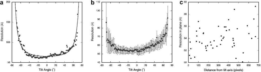
Resolution analysis of a tomogram. (A) Estimation of the resolution of a tilt series with a FRC cutoff of 0.3. The fitted curve gives the relationship to the relative thickness of the specimen at various tilt angles: $r=43.2+9.5e^{\frac{1}{1.18\text{cos}(\alpha )}}$. (B) Average of the resolutions estimated from each of 50 particles extracted from a tomogram as a function of the tilt angle (FRC cutoff of 0.3). The bars indicate the standard deviation error. (C) Resolution of each particle in the 0° tilt micrograph as a function of the distance from the tilt axis (disregarding the depth of the particle in the tomogram volume).

The resolution is strongly dependent on the tilt angle (Figure 5A). This expected behavior is mainly related to the change in thickness with the angle, with the resolution decreasing rapidly at higher tilt angles where the beam passes through more of the specimen. Fitting equation 1 to the data in Figure 5A suggests that the estimated resolution follows the decrease in intensity due to specimen thickness, although the quantitative interpretation of the fitted coefficients may not have meaning. An interesting feature is the slight progressive decrease in resolution between −40° and 40°, giving a distinct asymmetric impression. A possible explanation is that this represents some of the beam damage as the dose accumulates through the tilt series.

In our example the in plane resolution for the whole tomogram is estimated around 65 Å. Since the tomogram contains several particles similar in structure, but sparsely arranged in the volume, questions arise (i) whether a global resolution analysis reflects the quality of the single particles in the tomogram, and (ii) whether the location of such particles with respect to the tilt axis affects their resolution. We then extracted 50 sub-tilt series, each one tailored around a particle. Figure 5B shows that on average the resolution estimated for these regions follow the same pattern as for the whole tomogram. However, their in plane resolution is significantly better (around 53 Å), as a result of restricting the analysis to the structure of interest, thus excluding regions that contain only noise. Regarding the spatial variation of the resolution within the tomogram, apparently there is only a weak relationship between the resolution of the particles and their distance from the tilt axis (Figure 5C), with in plane estimates ranging from 50 to 60 Å. The alignments of the extracted particles were not refined, which may be one way to actually improve the resolution of subvolume reconstructions in the future.

3.4 Filtering and Denoising

Raw cryo-tomograms are inevitably contaminated by noise. Bsoft now embodies utilities that allow noise reduction in several ways.

3.4.1 Filtering out fiducial markers

The strong streaking that emanates from gold markers as well as negative interference effects in their immediate vicinity impacts adversely on the interpretability of density in these portions of a tomogram. This problem may be largely overcome by eliminating the markers after they have served their purpose for alignment, by substituting them in the projections by uniform density matched to the local average (Figure 6C). Only the markers used for alignment are removed, which typically covers all them except those close to the edges of the field and those coming into view only at higher tilt angles. If there is a need to remove markers not selected for alignment, more markers can be picked in bshow in the original tilt series.

3.4.2 Denoising filters

A limited improvement in signal-to-noise ratio may be achieved by various denoising filters. A comparison of the three filters implemented in Bsoft is illustrated in Figure 7 as applied to a tomographic reconstruction of an HSV capsid after symmetrization. The results vary in detail, and the choice of denoising method remains a subjective one.

Figure 7.

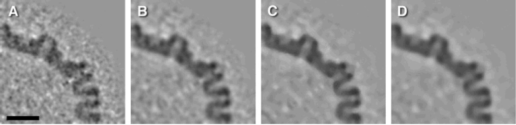
Noise reduction using different denoising methods. One HSV-1 capsid was extracted from a tomogram and 60-fold symmetrized. (A) Central section of capsid after symmetrization. (B–D) Central section of capsid after symmetrization and denoising with different filters: (B) bilateral filter, (C) median filter (three iterations), (D) anisotropic non-linear diffusion (60 iterations). Bar: 50 nm.

3.4.3 Denoising by symmetrization

A particle with symmetry can be oriented to a standard view (Heymann et al., 2005) and symmetrized to decrease noise. A HSV1 capsid with icosahedral symmetry was oriented to a reference map calculated by single particle analysis (Trus et al., 1996) and symmetrized (Figure 7A). If the symmetry is known but a reference map is not available, the symmetry axes can also be found and the particle correctly oriented for symmetrization.

3.4.4 Three-dimensional correlation averaging

Unless the structure is already known, it is not, in general, possible to distinguish between the respective contributions of signal and noise to densities recorded in a tomogram. Thus major improvements in SNR – and consequently, in resolution - are to be accomplished only by averaging features that are supposedly alike. The noise contributions, being random, will thereby be suppressed whereas the signal contributions, being consistent, will be maintained. This procedure is the three-dimensional equivalent of the long-standing practice of two-dimensional correlation averaging in electron microscopy (Frank, 1975). Procedures have been implemented in Bsoft that allow the picking of particles (subvolumes) from tomograms by hand, and their mutual translational and orientational alignment, with due accommodation for potential biasing by the ‘missing wedge’ effect (Frangakis et al., 2002).

4 Conclusion

The introduction of tomographic processing capabilities in Bsoft was motivated by the desire to provide more automated and effective tools to the community. The key elements provided are:

1. A workflow coupled to a flat file database for parameter management.

2. A fiducial-based alignment that is mostly automated and relatively robust.

3. A reconstruction algorithm with fewer artifacts than the commonly used weighted backprojection.

4. Implementation of a resolution-determination algorithm.

5. Methods to decrease noise through filtering and averaging approaches.

The Bsoft package has been tested on many different Unix-based platforms as well as VMS, and is available free of charge from http://Bsoft.ws.

Table 1.

Programs in Bsoft for use in tomography

Program	Use
btomo	General setup for a tomographic tilt series
bshow	Interactive image display with a setup for tomography
bnorm	Tomographic tilt series normalization
btrack	Fiducial marker tracking and refinement
bmgft	Generation of Fourier transforms and associated parameter files
btomrec	Tomogram reconstruction, full or in slabs
bzfft	Concatenation of slabs generated by btomrec and backtransform
btomres	Estimation of the resolution of a tomographic tilt series
bnad	Non-linear anisotropic diffusion filter
bbif	Bilateral filter
bmedian	Iterative median filter
btile	Splitting a big image into overlapping tiles
bpatch	Reassembling overlapping tiles into a single image
bpick	Extraction of particles/sub-volumes
bsubvol	Tracking sub-volumes in a tilt series
bfind	Reference-based orientation of 3D sub-volumes
badd	Weighted averaging of images

Table 2.

C-shell scripts for user convenience and distributed processing

Script	Programs used	Use
tomax	btrack	Determining the tilt axis angle
tomrec	bmgft, btomrec, bzfft	Piece-wise large tomogram reconstruction
tomres	bmgft, btomres	Resolution determination
tomnad	btile, bnad, bpatch	Piece-wise large tomogram denoising

Abbreviations

2D

two-dimensional

3D

three-dimensional

EM

electron microscopy

ET

electron tomography

STAR

self-defining text archiving and retrieval.

Appendix

Error calculations

The general problem to be solved in aligning a tilt series with fiducial markers is:

$${\overline{x}}_{ij}=A_i{\overline{g}}_j+{\overline{t}}_i$$ (1)

where $\overline{x_{ij}}$ is the location of a point or marker j in micrograph i, $\overline{g_j}$ is the location of the corresponding point j in 3D space, A_i is the 2×3 affine transformation matrix and $\overline{t_i}$ is the translation for micrograph i. The error for a point or marker j in a solution of (1) is:

$$\overline{{\epsilon }_{ij}}=\overline{x_{ij}}-A_i\overline{g_j}-\overline{t_i}$$ (2)

and the overall root-mean-square-deviation (RMSD) is then:

$$R=\sqrt{\frac{1}{nm}{\displaystyle \sum _i{\left|\overline{{\epsilon }_{ij}}\right|}^2}}$$ (3)

for n micrographs and m points or markers. Here the points are used in pixel coordinates and thus the RMSD gives a distance in pixels. Modified forms of (3) are used to determine the error for each marker (summing over all n micrographs) and the error per micrograph (summing over all m markers).

Tilt geometry

The common way of describing the tilt series geometry is somewhat different in terms of the Euler angles used than the description for the view as defined in Heymann et al. (Heymann et al., 2005). The tilt angles range from −90° to 90°, while the corresponding Euler angle, θ, ranges from 0° to 180°.

Given the nominal angles for the tilt series, the view is calculated from the tilt angle, α_t, and tilt axis angle, α_a:

$$\begin{array}{c}{v}_x=-\text{sin}{\alpha }_a\text{sin}{\alpha }_t\hfill \\ v_y=\text{cos}{\alpha }_a\text{sin}{\alpha }_t\hfill \\ v_z=\cos {\alpha }_t\hfill \\ v_a=0\hfill \end{array}$$

The corresponding standard Euler angles are:

$$\begin{array}{c}\theta =\{\begin{array}{c}{\alpha }_t\mathit{\text{if}}{\alpha }_t\ge 0\\ 180\mathrm{Ϸ}+{\alpha }_t\mathit{\text{if}}{\alpha }_t<0\end{array}\hfill \\ \varphi =\{\begin{array}{c}{\alpha }_a+\frac{\pi }{2}\mathit{\text{if}}{\alpha }_t\le 0\\ {\alpha }_a+\frac{\pi }{2}\mathit{\text{if}}{\alpha }_t>0\end{array}\hfill \\ \varphi =-\phi \hfill \end{array}$$

Note that there is some ambiguity in defining geometry: If the user chooses to define the tilt axis 180° from the convention used here, or if the user choose to switch the sign on the tilt angles, the resultant tomogram will be mirrored.

After refinement of the views, the tilt axis may not lie in the xy plane any more. The refined rotation matrix for each micrograph is converted into an axis vector, a, and tilt angle, α_t, and the new tilt axis angle and level angle calculated as:

$$\begin{array}{c}{\alpha }_a=\text{arctan}\frac{a_y}{a_x}\hfill \\ {\alpha }_l=\text{arcsin}{\alpha }_z\hfill \end{array}$$

The tilt axis angle, α_a, should be within 90° of the original user-defined tilt axis angle, if not, it must be adjusted by 180° and the tilt angle, α_t, negated. These angles are produced mainly for feedback to the user, and are never used internally in Bsoft.

Central section reconstruction for resolution estimation

In the resolution determination algorithm, we use the central section theorem to do a 2D reconstruction corresponding to a specific micrograph in the tilt series. Each central section is reconstructed including data ±1 reciprocal space voxel normal to the section. The contributions of other micrographs to that section is based on the transformation of the coordinates for a micrograph, $\overline{k_i}$, into the corresponding coordinates for the reconstruction image or central section, $\overline{k_r}$, is given by:

$$\overline{k_r}={\left(\overline{s}{M}_i\right)}^T{M}_r\overline{k_i}+\left(1-\frac{v_{i,z}}{v_{r,z}}\right)\frac{\overline{u_i}•\overline{k_i}}{\left|\overline{u_i}\right|}$$ (4)

The first term represents a rotation to the reference view using the matrix, M_r, a back rotation with the transpose of M_i, scaled by the tomogram size (typically the x and y sizes of the micrographs, and the thickness of the tomogram). The second term adjusts for the electron beam not being perpendicular to the plane of the reconstruction image. The offset is proportional to the micrograph coordinates, $\overline{k_i}$, and perpendicular to the tilt axis, defined by a unit vector that can be derived from normalized x and y coordinates of the view vector, $\overline{u_i}=\left\{v_{i,x},v_{i,y},0\right\}$. The adjustment is also a function of the separation of the two image planes as given by $1-\frac{v_{i,z}}{v_{r,z}}$, where v_i,z and v_r,z are the z-components of the view vectors for the micrograph and the reconstruction image, respectively. Note that the view vector, $\overline{v_i}$, is derived from the rotation matrix, M_i, and is therefore not independent of it. This treatment is approximate in the sense that deviation of the tilt axis from the xy plane is ignored.

References

- Baumeister W, Steven AC. Macromolecular electron microscopy in the era of structural genomics. Trends Biochem Sci. 2000;25:624–631. doi: 10.1016/s0968-0004(00)01720-5. [DOI] [PubMed] [Google Scholar]
- Brandt SS, Ziese U. Automatic TEM image alignment by trifocal geometry. J Microsc. 2006;222:1–14. doi: 10.1111/j.1365-2818.2006.01545.x. [DOI] [PubMed] [Google Scholar]
- Cantele F, Zampighi L, Radermacher M, Zampighi G, Lanzavecchia S. Local refinement: An attempt to correct for shrinkage and distortion in electron tomography. J Struct Biol. 2007;158:59–70. doi: 10.1016/j.jsb.2006.10.015. [DOI] [PMC free article] [PubMed] [Google Scholar]
- Cardone G, Grunewald K, Steven AC. A resolution criterion for electron tomography based on cross-validation. J Struct Biol. 2005;151:117–129. doi: 10.1016/j.jsb.2005.04.006. [DOI] [PubMed] [Google Scholar]
- Cardone G, Winkler DC, Trus BL, Cheng N, Heuser JE, Newcomb WW, Brown JC, Steven AC. Visualization of the herpes simplex virus portal in situ by cryo-electron tomography. Virology. 2007;361:426–434. doi: 10.1016/j.virol.2006.10.047. [DOI] [PMC free article] [PubMed] [Google Scholar]
- Diez DC, Seybert A, Frangakis AS. Tilt-series and electron microscope alignment for the correction of the non-perpendicularity of beam and tilt-axis. J Struct Biol. 2006;154:195–205. doi: 10.1016/j.jsb.2005.12.009. [DOI] [PubMed] [Google Scholar]
- Feja B, Aebi U. Determination of the inelastic mean free path of electrons in vitrified ice layers for on-line thickness measurements by zero-loss imaging. J Microsc. 1999;193:15–19. doi: 10.1046/j.1365-2818.1999.00436.x. [DOI] [PubMed] [Google Scholar]
- Frangakis AS, Hegerl R. Noise reduction in electron tomographic reconstructions using nonlinear anisotropic diffusion. J Struct Biol. 2001;135:239–250. doi: 10.1006/jsbi.2001.4406. [DOI] [PubMed] [Google Scholar]
- Frangakis AS, Bohm J, Forster F, Nickell S, Nicastro D, Typke D, Hegerl R, Baumeister W. Identification of macromolecular complexes in cryoelectron tomograms of phantom cells. Proc Natl Acad Sci U S A. 2002;99:14153–14158. doi: 10.1073/pnas.172520299. [DOI] [PMC free article] [PubMed] [Google Scholar]
- Frank J. Averaging of low exposure electron micrographs of non-periodic objects. Ultramicroscopy. 1975;1:159–162. doi: 10.1016/s0304-3991(75)80020-9. [DOI] [PubMed] [Google Scholar]
- Grunewald K, Desai P, Winkler DC, Heymann JB, Belnap DM, Baumeister W, Steven AC. Three-dimensional structure of herpes simplex virus from cryo-electron tomography. Science. 2003;302:1396–1398. doi: 10.1126/science.1090284. [DOI] [PubMed] [Google Scholar]
- Harris A, Cardone G, Winkler DC, Heymann JB, Brecher M, White JM, Steven AC. Influenza virus pleiomorphy characterized by cryoelectron tomography. Proc Natl Acad Sci U S A. 2006;103:19123–19127. doi: 10.1073/pnas.0607614103. [DOI] [PMC free article] [PubMed] [Google Scholar]
- Heymann JB. Bsoft: image and molecular processing in electron microscopy. J Struct Biol. 2001;133:156–169. doi: 10.1006/jsbi.2001.4339. [DOI] [PubMed] [Google Scholar]
- Heymann JB, Belnap DM. Bsoft: Image processing and molecular modeling for electron microscopy. J Struct Biol. 2007;157:3–18. doi: 10.1016/j.jsb.2006.06.006. [DOI] [PubMed] [Google Scholar]
- Heymann JB, Chagoyen M, Belnap DM. Common conventions for interchange and archiving of three-dimensional electron microscopy information in structural biology. J Struct Biol. 2005;151:196–207. doi: 10.1016/j.jsb.2005.06.001. (Corrigendum, J Struct Biol 153, 312) [DOI] [PubMed] [Google Scholar]
- Heymann JB, Winkler DC, Yim Y-I, Eisenberg E, Greene LE, Steven AC. CD Microscopy & Microanalysis 2006 Meeting. Navy Pier, Chicago: Cambridge University Press; 2006. Visualizing the Clathrin and Assembly-Regulating Proteins of Coated Vesicles by Cryo-Electron Tomography; p. 374. [Google Scholar]
- Iwasaki K, Mitsuoka K, Fujiyoshi Y, Fujisawa Y, Kikuchi M, Sekiguchi K, Yamada T. Electron tomography reveals diverse conformations of integrin alphaIIbbeta3 in the active state. J Struct Biol. 2005;150:259–267. doi: 10.1016/j.jsb.2005.03.005. [DOI] [PubMed] [Google Scholar]
- Jiang W, Baker ML, Wu Q, Bajaj C, Chiu W. Applications of a bilateral denoising filter in biological electron microscopy. J Struct Biol. 2003;144:114–122. doi: 10.1016/j.jsb.2003.09.028. [DOI] [PubMed] [Google Scholar]
- Kak AC, Slaney M. Principles of Computerized Tomographic Imaging. New York: IEEE Press; 1988. [Google Scholar]
- Kremer JR, Mastronarde DN, McIntosh JR. Computer visualization of three-dimensional image data using IMOD. J Struct Biol. 1996;116:71–76. doi: 10.1006/jsbi.1996.0013. [DOI] [PubMed] [Google Scholar]
- Lawrence A, Bouwer JC, Perkins G, Ellisman MH. Transform-based backprojection for volume reconstruction of large format electron microscope tilt series. J Struct Biol. 2006;154:144–167. doi: 10.1016/j.jsb.2005.12.012. [DOI] [PubMed] [Google Scholar]
- Ludtke SJ, Baldwin PR, Chiu W. EMAN: semiautomated software for high-resolution single-particle reconstructions. J Struct Biol. 1999;128:82–97. doi: 10.1006/jsbi.1999.4174. [DOI] [PubMed] [Google Scholar]
- Marabini R, Herman GT, Carazo JM. 3D reconstruction in electron microscopy using ART with smooth spherically symmetric volume elements (blobs) Ultramicroscopy. 1998;72:53–65. doi: 10.1016/s0304-3991(97)00127-7. [DOI] [PubMed] [Google Scholar]
- Mastronarde DN. Automated electron microscope tomography using robust prediction of specimen movements. J Struct Biol. 2005;152:36–51. doi: 10.1016/j.jsb.2005.07.007. [DOI] [PubMed] [Google Scholar]
- Nickell S, Forster F, Linaroudis A, Net WD, Beck F, Hegerl R, Baumeister W, Plitzko JM. TOM software toolbox: acquisition and analysis for electron tomography. J Struct Biol. 2005;149:227–234. doi: 10.1016/j.jsb.2004.10.006. [DOI] [PubMed] [Google Scholar]
- Penczek P, Radermacher M, Frank J. Three-dimensional reconstruction of single particles embedded in ice. Ultramicroscopy. 1992;40:33–53. [PubMed] [Google Scholar]
- Penczek PA, Renka R, Schomberg H. Gridding-based direct Fourier inversion of the three-dimensional ray transform. J Opt Soc Am A Opt Image Sci Vis. 2004;21:499–509. doi: 10.1364/josaa.21.000499. [DOI] [PubMed] [Google Scholar]
- Radermacher M, Wagenknecht T, Verschoor A, Frank J. A new 3-D reconstruction scheme applied to the 50S ribosomal subunit of E. coli. J Microsc. 1986;141:RP1–RP2. doi: 10.1111/j.1365-2818.1986.tb02693.x. [DOI] [PubMed] [Google Scholar]
- Ress D, Harlow ML, Schwarz M, Marshall RM, McMahan UJ. Automatic acquisition of fiducial markers and alignment of images in tilt series for electron tomography. J Electron Microsc (Tokyo) 1999;48:277–287. doi: 10.1093/oxfordjournals.jmicro.a023679. [DOI] [PubMed] [Google Scholar]
- Sandberg K, Mastronarde DN, Beylkin G. A fast reconstruction algorithm for electron microscope tomography. J Struct Biol. 2003;144:61–72. doi: 10.1016/j.jsb.2003.09.013. [DOI] [PubMed] [Google Scholar]
- Subramaniam S, Milne JL. Three-dimensional electron microscopy at molecular resolution. Annu Rev Biophys Biomol Struct. 2004;33:141–155. doi: 10.1146/annurev.biophys.33.110502.140339. [DOI] [PubMed] [Google Scholar]
- Trus BL, Booy FP, Newcomb WW, Brown JC, Homa FL, Thomsen DR, Steven AC. The herpes simplex virus procapsid: structure, conformational changes upon maturation, and roles of the triplex proteins VP19c and VP23 in assembly. J Mol Biol. 1996;263:447–462. doi: 10.1016/s0022-2836(96)80018-0. [DOI] [PubMed] [Google Scholar]
- van der Heide P, Xu XP, Marsh BJ, Hanein D, Volkmann N. Efficient automatic noise reduction of electron tomographic reconstructions based on iterative median filtering. J Struct Biol. 2006 doi: 10.1016/j.jsb.2006.10.030. in press. [DOI] [PubMed] [Google Scholar]
Associated Data
This section collects any data citations, data availability statements, or supplementary materials included in this article.