Game theory and reciprocity in some extensive form experimental games

Abstract

We examine decision making in two-person extensive form game trees using nine treatments that vary matching protocol, payoffs, and payoff information. Our objective is to establish replicable principles of cooperative versus noncooperative behavior that involve the use of signaling, reciprocity, and backward induction strategies, depending on the availability of dominated direct punishing strategies and the probability of repeated interaction with the same partner. Contrary to the predictions of game theory, we find substantial support for cooperation under complete information even in various single-play treatments.

We use variations on a relatively transparent, two-person extensive form bargaining game to examine principles of self-evident play (1) using experimental analysis. Our game is transparent if players can be expected to understand the relationship between the possible sequences of plays with their counterpart and the resulting payoffs which can be achieved. However, developing strategy for a relatively transparent game may not be self-evident, since it requires players to be confident about their counterparts actions and reactions. So, when are players likely to be mutually confident?

Evolutionary psychology provides one approach to answering this question. Hoffman et al. (2) and the references therein give a more extended discussion of the role of evolutionary psychology in explaining many economics experiments that exhibit anomalous behavior relative to standard theory. While economic theory assumes that individuals employ general purpose consciously cognitive algorithms to optimize gains in any situation, evolutionary psychology assumes that individuals deploy domain-specific cognitive algorithms, with different algorithms being used for different situations, often in nonconscious ways. Economic theory disciplines our thinking by requiring behaviors that maximize individual utility, whereas evolutionary psychology disciplines our thinking by requiring blueprints for behavioral activity which adapt under natural selection. Of course the relative value of these blueprints from nature depends on their subsequent development by cultural interaction (nurture) and a continuing evaluation of behavioral success through experience.

In this paper we address the following question: Can we use principles from game theory, experimental economics, and evolutionary psychology to better understand what is self-evident to players playing our extensive form games?

Data and experiment instructions reported in this paper are available by request (http://www.econlab.arizona.edu).

Principles of Behavior

The fundamental principles that underpin the propositions we examine experimentally can be stated as follows:

(i) Nonsatiation: Players prefer more money to less.

(ii) Dominance: Given a choice between two strategies, one of which yields potential payoffs to a player that strongly dominate those of the other, the dominating strategy will be chosen.

(iii) Backwards induction: In a sequential-move game tree (as in Fig. 1), each player will analyze the game by applying the dominance principle to the last potential subgame, then the penultimate subgame, and so on back through the full game. (Note, in games played with perfect information, such as Fig. 1, every decision node begins a subgame.) This principle allows subjects to interpret the credibility of implied threats and promises.

Figure 1.

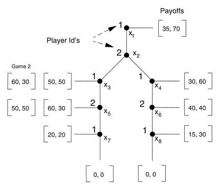
Game 1 in extensive form with initial vertex x₁. Players 1 and 2 take turns moving until a payoff box is reached. Player 1 receives the first amount, player 2 the second. Game 2 is identical to game 1 except the payoff boxes [60, 30] and [50, 50] are reversed.

Single-play game theory is about anonymous strangers, who meet once, interact strategically by applying the principles of dominance and backward induction, and never meet again (3, 4). These strong conditions are necessary to control for the effect of a history and a future external to the game in question but relevant to the current outcome. Without these controls on information, it would be extremely difficult to analyze a game with any confidence that the analysis can be restricted to that game.

(iv) The Folk theorem (reputations): Repeated play makes endogenous a history and a future that can be used to enforce threats, keep promises, and maintain credibility. Currently, game theory cannot predict repeated play outcomes, since a multiplicity of outcomes can be supported by some particular admissible trigger threat or punishment strategy. Neither can it predict which reputational equilibrium will occur. We will illustrate this below using game 1 in Fig. 1.

Repeated play, where players have incomplete information about the characteristics of their counterpart, enables players to build reputations as individuals with particular sets of characteristics (or types) who will punish or reward to achieve cooperation.

(v) Reciprocity: Contrary to the above principles, we can hypothesize that subjects exhibit a “habit of reciprocity”: a specialized mental algorithm (5, 6) in which long-term self-interest is best served by promoting an image both to others and yourself that cheating on cooperative social exchanges (either explicit or implicit) is punished (negative reciprocity), and initiation of cooperative social exchanges is rewarded (positive reciprocity). While some players may be sensitive to the difference between single and repeated game incentives in applying the reciprocity principle, other players will expect trust (cooperation without the option of punishing defection) to be rewarded by trustworthy responses even in single-play games. Still more players will initiate cooperation when defection can be punished, provided their own cost of punishment is not too high. Evolutionary psychology cannot currently predict the initial relative strength of the reciprocity algorithm within a player population, or the short-run stability of this behavior within a particular set of repeated interactions.

Experimental Design

In our experiments, we control for certain factors that either theory or empirical research suggests are likely to affect game-playing behavior. These factors are the presence or absence of the direct ability to punish noncooperative behavior and the protocol used to match players during repeat interactions. By varying these factors, we expect to learn under what conditions dominance or reciprocity is the mutually self-evident principle of play. There are many experiments where players fail to play dominating strategies; instead they seem to be using the principle of reciprocity. But these experiments typically do not offer players the choice between subgames where dominance alone is the principle of choice or subgames where reciprocity competes with dominance as the principle of choice. For example, in standard ultimatum (3) and investment (7) games, dominance clearly competes with reciprocity as the principle of choice, since there is no alternative for first movers except to make decisions that must be conditioned by the reciprocity of second movers. In our design, the second mover, who must make the decision whether or not to trust his counterpart (in some treatments) or to punish his counterpart (in other treatments), now has the option to choose instead a subgame where the dominance principle is self-evident.

The Constituent Games: Analysis and Payoff Issues.

The constituent games studied in this paper are shown in Fig. 1. A play of the game begins with player 1 moving at decision node x₁. Players alternate making moves down the game tree until a payoff box is reached. The player identification at the upper left of each decision node indicates which player moves at that node. The left number in each payoff box is player 1’s payoff, while the right number is player 2’s payoff. In the text we denote payoffs as ordered pairs with player 1’s payoff first and player 2’s payoff second. For example, if player 1 moves right at x₁ the game ends at the outcome with the maximum joint payoff, giving 35 to player 1 and 70 to player 2, denoted [35, 70].

In game 1 cooperation can lead to the largest symmetric outcome resulting in the payoffs [50, 50]. To reach [50, 50], player 2 must move left at x₂. But if player 2 moves left, player 1 can defect by moving down at x₃, making [60, 30] player 2’s best choice. Alternatively, player 2 could incur a costly choice and directly punish player 1 by choosing to move down in the subgame at x₅. But this direct punishment strategy is subgame dominated by the strategy of choosing left at x₅. This allows us to ask if subjects play subgame-dominated strategies. When the constituent game is repeated, players 2 can avoid playing dominated punishing strategies and follow an indirect, individually rational, trigger strategy: if player 1 defects in repetition t, then player 2 moves left at x₅, but right at x₂ in repetition t + 1, punishing player 1 with at least the subgame perfect outcome [40, 40], then, in repetition t + 2, returns to playing left at x₂. By using this strategy every time player 1 defects, player 2 avoids the more costly direct punishment outcome [20, 20]. But for player 1 to be made strictly worse off, player 2 must punish, or credibly threaten to punish, right at x₂ more than once for each defection, since a single punishment gives player 1 (60 + 40)/2 = 50.

Game 2 is identical to game 1, except that we have interchanged the payoffs [60, 30] and [50, 50], thus removing the threat of direct punishment. This allows us to ask if trust, unsupported by a direct punishment option, affects the frequency of cooperation. In either game 1 or 2, the anticipated failure of cooperation may result in player 2 moving right at x₂. Once player 2 moves right, player 1 should reason that it is in both their interests to reach [40, 40]. We will call this outcome SP, since it is the subgame perfect outcome (8). In both games, the cooperative outcome [50, 50] and SP outcome (40, 40) are symmetric, thus controlling for any payoff equity motivations in subject choice.

The above discussion and the questions we pose for experimental investigation make it clear why we selected the particular three payoffs on the left and the three on the right in constituent games 1 and 2. But why do we choose the play-stopping outcome [35, 70] at the top?

First, it provides an outside option that minimizes the multiple-move cost of transacting. Second, for player 1, it provides an outcome only five units inferior to the SP outcome. Therefore it may be a subjectively rational outcome. If players 1 in the population want to avoid tedious multiple moves, risk, and puzzling about what their player 2 counterparts will do and incur a “sure thing” opportunity cost of only five units, then we will observe lots of right moves at x₁. The relative payoffs available at top right allow one to examine the background conditions under which game theoretic analysis becomes relevant. Third, when any of the constituent games are repeated, top right is a Nash equilibrium under a strategy in which player 2 always moves right at x₂ and down at x₆. This gives player 1 the individually rational payoff 15, and the self-interested option to subsequently move right at x₁.

This leaves the outcomes [0, 0] at nodes x₇ and x₈ to be explained under repeated play. Since [20, 20] at x₇ and [15, 30] at x₈ constitute punishing payoffs, why do we add the vindictive outcome [0, 0] at both nodes? We interpret choosing down at x₇ or x₈ by player 1 as a form of escalation: “if you are going to choose a punishing strategy, I will simply counterpunish.” On the left, this is irrational escalation. If by moving down at x₇, player 1 is telling 2 not to punish, player 2 is not rationally going to learn to move left at x₂, then accept defection at x₃. Rather, player 2 seems more likely to conclude that player 1 is not educable; the rational lesson is to simply move right at x₂ on subsequent plays and avoid such escalation on the left side of the tree. At x₈, moving down may be a form of rational escalation in which player 1, seeing that player 2 is attempting to force a right move at x₁, signals that she is prepared to use deterrence tactics to neutralize player 2’s use of this strategy. Such counterpunishment is unlikely, since we think it unlikely that players 2 will use strategies designed to achieve [35, 70] in the first place.

Matching Protocols.

When Selten and Stoecker (9) randomly paired anonymous players in ten repeated plays of a prisoner’s dilemma game, they found that cooperation begins to unravel. This suggests that in the dominant strategy prisoner’s dilemma, experience causes players to update their beliefs by giving less weight to the existence of types who would cooperate. If they believe that it is more likely that their opponent is only pretending to be a cooperative type, then subjects defect sooner in anticipation of a defection by their counterparts. A similar slow convergence to the Nash equilibrium was found by McCabe (10) in a six-period fiat money game, and by Smith et al. (11) in a 15-period laboratory stock market. Thus, for finitely repeated games, there is a body of experimental literature that shows that the backward induction Nash equilibrium predicted by game theory does occur when players gain sufficient experience, and cooperation is strategically difficult or costly to attain. In this paper, we investigate players’ ability to cooperate in two-person extensive form games, under single play or repeated play where the length of the supergame is unknown.

We examine four matching protocols for pairing players when play is repeated. (Refer to Table 1). The protocol itself is always common information to all players. In single protocol, subjects play a randomly chosen counterpart once and then the experiment is over. The single play design allows us to ask if cooperation is possible without repeat interaction. Game theory predicts no: players should end at SP. But reciprocity theory implies that some players may be programmed by culture (or the biology of their minds) to attempt cooperation in single play as a habitual long-term strategy that increases the individual’s long-term payoff. In repeat single protocol, subjects play each counterpart in the population exactly once, with their own role alternating between player 1 and player 2. This protocol allows some learning about the sample while controlling, in theory, for repeated game effects. Again game theory predicts SP. In single 1 exp, experienced subjects from repeat single 1 return to the laboratory on a different day for a single-play session. Do increased experience and single-play conditions increase support for the game theoretic SP outcome?

Table 1.

Experimental design: Treatments and number of pairs

Designation	Constituent game	Matching protocol	No. pairs (observations)
Single 1	1	Single-play	26 (26)
Single 2	2	Single-play	26 (26)
Repeat single 1	1	Repeat single play*	24 (360)†
Single 1 exp	1	Single-play	17 (17)
Same 1	1	Repeat same pairs	22 (440)
Same 2	2	Repeat same pairs	23 (460)
Random 1	1	Repeat random pairs and roles	24 (480)†
Random 2	2	Repeat random pairs and roles	24 (480)†

^*Each player plays each counterpart exactly once, with role alternating between player 1 and 2. 

^†Sessions consist of 12 players, 6 pairs matched repeatedly. Others consisted of at least 8 players. 

In random matching, each time the constituent game is played, subjects are randomly assigned a role, player 1 or player 2, and are randomly paired. This protocol maximizes the number of possible role pairings for any fixed sample and makes it difficult to implement repeat game strategies, since such responses are diffused through the entire sample. In both repeat single and random matching, subjects remain anonymous and are not given their counterpart’s history.

In same pairings, subjects keep the same counterpart and role throughout play. This design maximizes the opportunity for coupling: learning about one’s counterpart and implementing repeated game strategies.

By considering behavior across the four protocols (single, repeat single, random, and same) using a between-players design, we can ask if cooperation improves as you increase the probability of playing the same counterpart as conjectured by the Folk theorem.

Treatments and Procedure.

Our treatments are summarized in Table 1. For convenience, we adopt the convention of naming a cell by the matching treatment and the number of the game. Thus, same 1 designates experiments where players keep the same counterpart and play game 1 repeatedly.

Players in repeated-play experiments are recruited for 2 hr, even though the experiment lasts only slightly over 1 hr. Players are not told how long the experiment will last; this makes credible the expectation of a long series of repeated plays. Players are paid $5.00 as a nonsalient show-up fee, and, at the end of the experiment, their accumulated earnings. The payoffs shown in the boxes are in cents for the constituent games that are repeated 20 times. In the single-play games, the payoffs are all multiplied by 20 to maintain payoff comparability with the repeated game experiments.

In the instructions we are careful to avoid using terms like “game,” “play,” “opponent,” “partner,” or other potentially suggestive, value-laden terminology. In particular, players are informed that they will participate in a two-person decision-making problem involving themselves and a counterpart who will be designated DM1 or DM2. Subjects are given computer-programmed practice in making moves and are able to observe the recording of moves and payoffs in a game unrelated to the game they are to play in the experiment. They are allowed to ask questions privately at any time during the instructions.

Subject’s decisions are executed via touch- or “mouse”-sensitive arrows, appearing in sequence in the game tree on their screen displays. This procedure is intended to help concentrate their attention on their screens.

Extending Bayesian Bernoulli Trials Theory

The data evaluations to follow will be based on conditional probabilities applied to a Bernoulli process—e.g., in Fig. 1, each player 2 in the sample can move right or left at node x₂, with prior uncertainty—to the experimenter—as to the probability p (right) and (1 − p) (left). This requires us to first extend the parameter space of standard Bernoulli trials theory to allow probability assessment of an extreme research hypothesis. Thus the strict game theoretic prediction is p = 1 for right play at node x₂ (also x₆). But the standard Bernoulli process generates the occurrence of r right outcomes in n independent trials, given p defined on the open interval 0 < p < 1. The situation is analogous to the possibility that a coin can be biased toward “heads” to any degree, including being two-headed (or two-tailed). If someone observes five heads in five trials, the coin cannot be two-tailed, but can be two-headed, biased, or even fair, since five straight heads rules out only the state of being two-tailed. With standard Bernoulli trials theory, we cannot conclude that this coin is two-headed: only that it is more or less biased toward heads. In the data below, we observe many cases in which n = r > 0 and n > r = 0 and will want to assess the probability that p = 1 or 0.

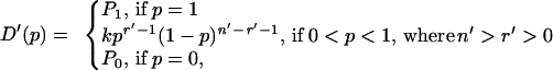
We denote by D′(p) anyone’s (the experimenter’s or the reader’s) uncertainty about p before experimentation. We let D′(p) be a beta density on (0 < p < 1), with parameters (r′,n′), P₀ > 0 be the prior probability that p = 0, and P₁ > 0 be the prior probability that p = 1. Clearly, in Fig. 1, a game theorist would associate some prior probability mass, P₁, with p = 1, the conditional probability that all players 2 will play right at x₂ in single 1. Likewise in the repeated game, same 1, the theorist would find it credible with some positive probability P₀ > 0 that all players 2 will move left at x₂. The prior mixed density/mass function is then:

1

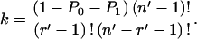
where P₀ + P₁ < 1. Since D′(p) must have unit measure over the set, we must have:

2

Note that if n′ = 2 and r′ = 1, then the beta density is rectangular, and k = 1 − P₀ − P₁, the constant density on (0 < p < 1).

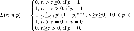
The likelihood of observing that r of n subjects move right, conditional on p, is then:

3

Eq. 3 states that if p = 1 (all players 2 would elect right at x₂ or x₆), then there is zero likelihood of observing r < n moves right, a certainty of observing n = r moves right, the binomial probabilities (r,n) for 0 < p < 1, and so on.

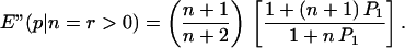
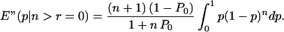
We next state the posterior distribution of p, D"(p|r,n), given the sample observation (r,n), which is proportional to the product of the kernels (the parts that are functions of p) of Eqs. 1 and 3. The factor of proportionality, which depends on (r,n), gives D" the property of the unit measure over (0 ≤ p ≤ 1). Using node x₂ for illustration, there are three cases, depending upon whether we observe both right and left moves, all right moves, or all left moves. In each case we will compute D", assuming that D"(p) = 1 − P₀ − P₁, or n′ = 2 and r′ = 1 in Eq. 1.

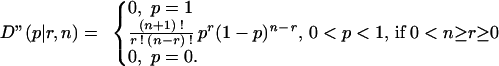4

Since both right and left are observed, none of the prior mass, P₀ or P₁, on the end points can affect the posterior. The result devolves to the standard Bernoulli process defined on 0 < p < 1.

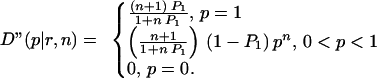5

Hence, as n = r gets large, we become increasingly sure that p = 1.

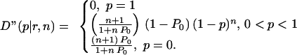6

Results: Posterior Expected Probabilities

Using the posterior probability functions Eqs. 4–6, we calculate the expected probabilities of observing (r,n) if the prior probability function Eq. 3 is rectangular, giving:

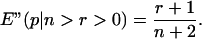7

8

9

The results applied to the outcome (r,n) in each game treatment are shown in Tables 2 and 3 for four hypotheses: (i) right versus left move at node x₂; (ii) right move at node x₆ (SP) versus all other outcomes in the right branch of game 1; (iii) down move in game 1, or left move in game 2, at node x₃ (defection from signal to cooperate) versus no defection; and (iv) down move in game 1 at node x₅ (punish defection) versus no punishment. In each case, we assume that P₀ = P₁ = 1/4, so that half the prior mass is divided equally between p = 0 and p = 1, while the other half is smeared over the interval 0 < p < 1. The reader is free to express his/her own prior beliefs, before examining Tables 2 and 3, then make the calculations from Eqs. 1–3.

Table 2.

Frequency of outcomes and conditional expected posterior probabilities: Single experiments

Treatment	Node x2, right (noncooperation)			Node x6, right (SP)			Node x3, down game 1 or left game 2 (defection)			Node x5, down game 1 (punish)
	n	r	E"(p|r,n)	n	r	E"(p|r,n)	n	r	E"(p|r,n)	n	r	E"(p|r,n)
Single 1	26	13	0.50	13	12	0.867	13	3	0.267	3	1	0.40
Single 2*	26	14	0.536	14	14	0.990	12	6	0.50	NA	NA	NA
Repeat single 1†	24	10	0.423	10	10	0.982	14	5	0.375	5	3	0.571
Single 1 exp‡	17	4	0.263	4	4	0.938	13	5	0.40	5	2	0.429

NA, not applicable. 

^*Note that in game 2, the move order of the outcomes [60, 30] and [50, 50] are reversed relative to game 1. 

^†Data for last trial only for comparability with other single experiments. 

^‡Seventeen of the 24 pairs from repeat single 1 returned for a single play of game 1 with a 20-fold increase in payoffs. 

Table 3.

Frequency of outcomes and conditional expected posterior probabilities: Repeated-play experiments

Treatment	Node x2, right (noncooperation)			Node x6, right (SP)			Node x3, down game 1 or left game 2 (defection)			Node x5, down game 1 (punish)
	n	r	E"(p|r,n)	n	r	E"(p|r,n)	n	r	E"(p|r,n)	n	r	E"(p|r,n)
Same 1	433	80	0.186	80	68	0.841	353	41	0.118	41	27	0.651
Same 2*	423	162	0.384	162	114	0.701	261	41	0.160	NA	NA	NA
Random 1	471	154	0.328	154	149	0.962	317	102	0.223	102	69	0.673
Random 2*	453	293	0.646	293	278	0.946	160	70	0.438	NA	NA	NA
Repeat single 1	352	148	0.421	148	138	0.927	204	71	0.375	71	36	0.507

NA, not applicable. 

^*Note that in game 2, the move order of the outcomes [60, 30] and [50, 50] are reversed relative to game 1. 

Single-Play Experiments.

Table 2 lists E"(p|r,n) for each of the nodal choice hypotheses i–iv corresponding to each single treatment.

Result 1. Right moves at x₂ (noncooperation) in game 1 are far less prevalent than implied by standard game theoretic analysis. The expected posterior probability of a right move at x₂ is 0.5 in game 1.

Result 2. Repetition of game 1 with distinct counterparts (repeat single 1) lowers the final trial probability of right moves at x₂ to 0.423. Experience and learning slightly favor cooperation. When 17 of the latter 24 subjects return for a single-play session (single 1 exp), right move probability declines further to 0.263. Essentially, they return for a single trial with a 20-fold increase in stakes and play it more like another round in the repeated game than a situation calling for noncooperative play.

Result 3. Trust accounts for almost all of the offers to cooperate by players 2, since removing the option to punish defection increases the frequency of right moves at x₂ only slightly. This is indicated by the observation that the posterior probability of right moves at x₂ in game 2 is 0.536 compared with 0.50 in game 1.

Result 4. Consistent with the prediction of game theory, there is a high probability of achieving the SP outcome, contingent on play being on the right branch of the tree in both games 1 and 2. Thus, the probability of SP varies from 0.867 (single 1) to 0.990 (single 2). (See Table 3 showing that this result is also supported in the repeated-play treatments).

Result 5. Contrary to the game theoretic prediction based on dominance, in all treatments the conditional probabilities of defection (player 1 moves down at x₃) from offers to cooperate (player 2 moves left at x₂) in game 1 are 0.4 or less.

The observation that dominance characterizes moves in the right tree (Result 4) but not in the left tree is clear evidence in favor of the reciprocity hypothesis, since only moves within the left tree can reflect reciprocity responses.

Result 6. In game 2, where defection (player 1 moves left at x₃) can occur without punishment, the defection probability rises from that in game 1, but only to 0.5 and is thus surprisingly low. This result together with Result 3 implies that trust and trustworthiness occur with about equal probability: the probability that a player 2 will offer to cooperate is 0.464 (Result 3), while the probability of a positive reciprocal response by a player 1 is 0.5. (See Table 3 showing that the higher defection rate in game 2 relative to game 1 applies also to the repeated-play treatments: same 2 versus same 1; random 2 versus random 1.)

Result 7. In game 1, the expected probability of punishment (player 2 moves down at x₅) is at least 0.4 across the three treatment conditions. This is contrary to the game theoretic prediction based on dominance but is consistent with the reciprocity hypothesis. Players 2, having offered to cooperate by left play at x₂, appear to feel some obligation in spite of the cost to themselves, to punish players 1 who defect. (See Table 3 showing that the conditional probability of punishment is at least 0.5 across all trials in the repeated-play treatments: same 1, random 1, and repeat single 1).

Repeated-Play Experiments.

Table 3 lists E"(p|n,r) for choice hypotheses i–iv corresponding to each repeated-play treatment.

Result 8. The Folk theorem that repeated play favors cooperation is supported; when the same pairs interact repeatedly (same 1), the probability of a right move at x₂ is 0.186, the lowest across all treatments. Similarly, comparing single 2 in Table 2 with same 2 in Table 3, repeated play increases cooperation in game 2 where the direct punishment option is not available.

Result 9. In game 1, as the probability of being matched with the same counterpart decreases from 1 to 0 across the three treatments, same 1, random 1, and repeat single 1, the probability of noncooperation (a right move at x₂) increases (0.186, 0.328, and 0.421, respectively). Similarly, in game 2, comparing same 2 with random 2, the probability of noncooperation increases from 0.384 to 0.646. This is qualitatively consistent with Folk theorem expectations.

Optimality and Efficiency of Player Choices

In Table 4, for all treatments we report calculations of the expected payoff to a player 2 of a left move at x₂, denoted E(π₂|Left). The calculations are based on the subsequent conditional likelihood probabilities of actual game play. Since the SP return to a player 2 from moving right at x₂ is 40, values of E(π₂|Left) >40 imply that left at x₂ increases the expected payoff to player 2. Conditional on a left move at x₂, we also calculate the expected payoff to a player 1, E(π₁|Down), of defecting (moving down at x₃) in Game 1. If (π₁|Down) is >50 (the return if player 1 does not defect), then defection is a best choice. Efficiency, appearing in the last column for each treatment, is the expected payoff, to a pair of subjects based upon observed conditional likelihoods from game play (beyond node x₂) divided by the cooperative joint payoff (50 + 50 = 100). Thus, an efficiency of 80% implies that the individual pairs receive an average return equal to the SP joint payoff (40 + 40 = 80).

Table 4.

Expected profits from a left move at x₂ and from defection

Treatment	E(π2|Left)*	E(π1|Down)†	Efficiency‡, %
Single 1	44.6	46.7	85.5
Single 2§	40.0	NA	86.9
Single 1 exp*	40.7	44.0	86.4
Same 1	46.6	31.3	90.6
Same 2§	46.9	na	90.3
Random 1	40.7	30.8	82.6
Repeat single 1	41.5	42.0	85.1
Random 2§	41.2	NA	84.7

NA, not applicable. 

^*Expected payoff to player 2 from moving left at x₂, given the relative frequencies of subsequent play by player 1s and 2s. 

^†Expected payoff to player 1 from defecting at node x₃, game 1. 

^‡Efficiency is the percentage of the cooperative [50, 50] total payoff that is realized by all pairs. 

^§Note that in game 2, the move order of the outcomes [60, 30] and [50, 50] are reversed relative to game 1. 

Result 10. From the first column of data in Table 4, it is clear that players 2 who move left at x₂ earn a higher return than those moving right for the SP outcome. This is the case for all the treatments whether single or repeated play. Even Single 2 achieves an expected payoff of 40 on the left, equal to the SP payoff. The message is that those players who move left at x₂ are, on average, reading their counterparts correctly. It pays to initiate acts that invite positive reciprocity (trust), because such acts tend to be rewarded by positive reciprocation (trustworthiness), particularly when the invitation is reinforced by the option of punishing defection.

Result 11. Referring to the second column of entries in Table 4 for E(π₁|Down), it is seen that defection never pays. The defector, player 1, in all treatments receives a return <50. The claim by Cosmides (5) that people’s mental modules are programmed to punish cheaters is alive and well in our experiments. Defection is not always punished, but it is often enough to keep defection from being profitable.

Result 12. In all treatments, players jointly achieve more efficient outcomes—they collect more money from the experimenter—than is predicted by noncooperative game theory.

Evolution of Game Play over Repetitions

Tables 5–9 report conditional likelihood probabilities, aggregated over blocks of five repetitions each, for each payoff outcome corresponding to the repeated-play experiments.

Table 5.

Conditional outcome probabilities by repetition block repeat single 1

Repetitions	Conditional outcome probabilities*
	Left branch†	50 50	60 30	20‡ 20	Right branch†	30 60	40 40	15‡ 30	E(πx|Left)	E(π1|Down)
1–5	68/116	43/68	12/25	13/13	48/116	7/48	41/41	0	40.7	39.2
	= 0.586	= 0.632	= 0.48	= 1	= 0.414	= 0.146	=1
6–10	71/117	46/71	15/25	10/10	46/117	2/46	43/44	0/1	41.6	44.0
	= 0.607	= 0.648	= 0.60	=1	= 0.393	= 0.043	= 0.977	= 0
11–15	65/119	44/65	8/21	13/13	54/119	0/54	54/54	0	41.4	35.2
	= 0.546	= 0.677	= 0.381	= 1	= 0.454	= 0	= 1

^*The conditional probabilities are likelihoods, based on (r/n) = (realizations/no. of observations). 

^†Moves right at x₁ ending with payoff [35, 70] can be inferred from the left and right branch denominators shown in these entries—e.g., 116 of 120 moved right or left in repetition blocks 1–5, implying that four pairs ended at [35, 70]. 

^‡Moves ending with payoffs [0, 0] at these nodes can be inferred from these entries—e.g., if 0 of 1 end at [15, 30], then 1 of 1 ended at [0, 0]. 

Result 13. In repeat single 1 (Table 5), there is no obvious and important trend in any of the outcomes, although in the last repetition block, the probability of punishment increases and the return from defection declines. It is not possible to say that players are “learning to play SP” over time. Neither are they learning to cooperate, although in every block the average return to a left move at x₂ is >40.

Result 14. In same 1 (Table 6), left moves at x₂ followed by cooperation starts high and trends upward across repetitions, while support for right moves to SP declines. Defection declines only slightly across repetitions blocks. More interesting is that punishment begins at a modest 57% (8 in 14) in the first five repetitions, then increases to over 91% (11 in 12) in the next five repetitions, and goes through a similar cycle in the last two blocks. It appears that defection is at first tolerated—players 2 are forgiving—then punishment is strongly invoked, and the effect is to reduce total defection from 14 to only 8 in the last block as defectors find that it does not pay.

Table 6.

Conditional outcome probabilities by repetition block same 1

Repetitions	Conditional outcome probabilities*
	Left branch†	50 50	60 30	30‡ 20	Right branch†	30 60	40 40	15‡ 30	E(π2|Left)	E(π1|Down)
1–5	78/109	64/78	6/14	8/8	31/109	2/31	28/29	0/1	45.4	37.2
	= 0.716	= 0.821	= 0.429	= 1	= 0.284	= 0.065	= 0.966	= 0
6–10	88/108	76/88	1/12	7/11	20/108	0/20	19/20	0/1	45.1	16.6
	= 0.815	= 0.864	= 0.083	= 0.636	= 0.185	= 0	= 0.95	= 0
11–15	94/106	87/94	4/7	3/3	12/106	0/12	12/12	0	48.2	42.8
	= 0.887	= 0.926	= 0.571	= 1	= 0.113	= 0	= 1
16–20	93/110	85/93	3/8	4/5	17/110	1/17	9/16	4/7	47.5	32.5
	= 0.845	= 0.914	= 0.375	= 0.8	= 0.155	= 0.059	= 0.563	= 0.571

^*The conditional probabilities are likelihoods, based on (r/n) = (realizations/no. of observations). 

^†Moves right at x₁ ending with payoff [35, 70] can be inferred from the left and right branch denominators shown in these entries—e.g., 116 of 120 moved right or left in repetition blocks 1–5, implying that four pairs ended at [35, 70]. 

^‡Moves ending with payoffs [0, 0] at these nodes can be inferred from these entries—e.g., if 0 of 1 end at [15, 30], then 1 of 1 ended at [0, 0]. 

Result 15. In same 2 (Table 7), the proportion of left moves at x₂ starts at only 0.45, much lower than in same 1 (0.716), and rises steadily to 0.743 in the last five repetitions; defection declines correspondingly. Hence, the substantial role of trust in achieving cooperation through reciprocity when the same pairs meet repeatedly. The expected profit from moving left at x₂ rises steadily from 42.9 to 48.2 across all blocks.

Table 7.

Conditional outcome probabilities by repetition block same 2

Repetitions	Conditional outcome probabilities*
	Left branch†	60 30	50 50	20‡ 20	Right branch†	30 60	40 40	15‡ 30	E(π2|Left)
1–5	45/100	16/45	29/29	0	55/100	7/55	42/48	6/6	42.9
	= 0.450	= 0.356	= 1		= 0.550	= 0.127	= 0.875	= 1
6–10	65/110	10/65	55/55	0	45/110	11/45	26/34	8/8	46.9
	= 0.591	= 0.154	= 1		= 0.409	= 0.244	= 0.765	= 1
11–15	73/108	8/73	65/65	0	35/108	6/35	23/29	6/6	47.8
	= 0.676	= 0.110	= 1		= 0.324	= 0.171	= 0.793	= 1
16–20	78/105	7/78	71/71	0	27/105	3/27	23/24	1/1	48.2
	=0 .743	= 0.090	= 1		= 0.257	= 0.111	= 0.952	= 1

^*The conditional probabilities are likelihoods, based on (r/n) = (realizations/no. of observations). 

^†Moves right at x₁ ending with payoff [35, 70] can be inferred from the left and right branch denominators shown in these entries—e.g., 116 of 120 moved right or left in repetition blocks 1–5, implying that four pairs ended at [35, 70]. 

^‡Moves ending with payoffs [0, 0] at these nodes can be inferred from these entries—e.g., if 0 of 1 end at [15, 30], then 1 of 1 ended at [0, 0]. 

Result 16. The proportion of left moves at x₂ in random 1 (Table 8) begins at 0.624 and rises to 0.746, uniformly below the corresponding results in same 1 (Table 6), and demonstrating the game-theoretic Folk principle that the same counterparts can better coordinate cooperation. Defections are higher in random 1 than in same 1, but, in random 1, players 2 tend to persist in left moves at x₂ but increase their punishment rates: without the same role and pairs, players 2 encounter many more defecting counterparts but proceed to incur the personal cost of punishing them. This strengthens the results in Cosmides (5), where cheaters are punished, but at no cost to the punisher.

Table 8.

Conditional outcome probabilities by repetition block random 1

Repetitions	Conditional outcome probabilities*
	Left branch†	50 30	60 30	20‡ 20	Right branch†	30 60	40 40	15‡ 30	E(π2|Left)	E(π1|Down)
1–5	73/117	47/73	15/26	10/11	44/117	0/44	44/44	0	41.1	42.3
	= 0.624	= 0.644	= 0.577	= 0.909	= 0.376	= 0	= 1
6–10	78/117	50/78	8/28	17/20	39/117	0/39	37/39	1/2	39.5	29.3
	= 0.667	= 0.641	= 0.286	= 0.85	= 0.333	= 0	= 0.949	= 0.5
11–15	78/119	51/78	6/27	17/21	41/119	1/41	38/40	2/2	39.4	25.9
	= 0.655	= 0.654	= 0.222	= 0.810	= 0.345	= 0.024	= 0.95	= 1
16–20	88/118	67/88	4/21	14/17	30/118	0/30	30/30	0	42.6	24.7
	= 0.746	= 0.761	= 0.190	= 0.824	= 0.254	= 0	= 1

^*The conditional probabilities are likelihoods, based on (r/n) = (realizations/no. of observations). 

^†Moves right at x₁ ending with payoff [35, 70] can be inferred from the left and right branch denominators shown in these entries—e.g., 116 of 120 moved right or left in repetition blocks 1–5, implying that four pairs ended at [35, 70]. 

^‡Moves ending with payoffs [0, 0] at these nodes can be inferred from these entries—e.g., if 0 of 1 end at [15, 30], then 1 of 1 ended at [0, 0]. 

Result 17. Random 2 yields lower likelihoods of left play (Table 9) than same 2 (Table 7) in every repetition block, and the modest growth in left play to 0.405 drops to 0.330 in the final block. Initially, the expected profit from left play is high then declines. This correlates with a modest increase in left game play in repetitions 6–10 and 11–15, but defections increase in these blocks, and the expected return from left play falls, leading to a decline in left game play in repetitions 16–20.

Table 9.

Conditional outcome probabilities by repetition block random 2

Repetitions	Conditional outcome probabilities*
	Left branch†	60 30	50 50	20‡ 20	Right branch†	30 60	40 40	15‡ 30	E(π2|Left)
1–5	32/110	9/32	23/23	0	78/110	4/78	73/74	0/1	44.4
	= 0.291	= 0.281	= 1		= 0.709	= 0.051	= 0.986	= 0
6–10	43/112	17/34	26/26	0	62/112	0/69	66/69	2/3	42.1
	= 0.384	= 0.395	= 1		= 0.616	= 0	= 0.957	= 0.667
11–15	47/116	26/47	21/21	0	69/116	1/69	66/68	2/2	38.9
	= 0.405	= 0.553	= 1		= 0.595	= 0.014	= 0.971	= 1
16–20	38/115	18/38	20/20	0	77/115	2/77	73/75	0/2	40.5
	= 0.330	= 0.474	= 1		= 0.670	= 0.026	= 0.973	= 0

^*The conditional probabilities are likelihoods, based on (r/n) = (realizations/no. of observations). 

^†Moves right at x₁ ending with payoff [35, 70] can be inferred from the left and right branch denominators shown in these entries—e.g., 116 of 120 moved right or left in repetition blocks 1–5, implying that four pairs ended at [35, 70]. 

^‡Moves ending with payoffs [0, 0] at these nodes can be inferred from these entries—e.g., if 0 of 1 end at [15, 30], then 1 of 1 ended at [0, 0]. 

Other Results

Generally, players 1 move down at x₁. Thus in repeat single 1, of 360 constituent game plays (See Table 1), 352 show right or left moves at x₂ (See Table 3), implying that only 8 moves by players 1 were right at x₁.

We also observe that moving down at x₆ is quite rare; it is most frequent in same 2 where 21 (not shown) out of a total of 460 plays of game 2 involve moving down at x₆. These appear to have been intended to induce a right move at x₁ on the subsequent play, since total moves right at x₁ were 37.

Do Trusting People Tend to Be Trustworthy?

In repeat single 1, subjects alternate between the roles of player 1 and player 2. Consequently, we have data on each subject in both positions, matched repeatedly against distinct persons. It is natural to hypothesize that, since subjects are matched anonymously from a particular population of like individuals (undergraduates), then each can consider themselves as a sample of size 1 from the characteristics of that population. If a person is a cooperative type and assumes that he/she is matched with a cooperative type, then offers to cooperate are expected to be reciprocated by cooperative responses. This assumes that trusting persons are also trustworthy (see discussion in Result 6). Do our data confirm this? That is, if a person in the player 2 role moves left, is that person, when in the player 1 role, less likely to be a defector in the left tree? Similarly, is a person who moves right as a Player 2, likely to be a defector as player 1 in the left tree?

The results from repeat single 1 are compiled in Table 10. There were 48 subjects (24 pairs). One subject never recorded an outcome in the left tree branch as player 1. The remaining 47 recorded left branch outcomes in each role at least once, and the joint relative frequencies for the choices (cooperate as player 2, reciprocate as player 1) corresponding to moves left at x₂, and left at x₃, are shown in Table 10 aggregated by one-thirds. Thus, 21.2% of the subjects exhibit the lowest frequency, 0–0.33, of cooperation and reciprocation. In the upper right corner, the modal outcome 29.8%, falls into the highest frequency range of cooperation/reciprocation. As expected, if trust goes with trustworthiness and vice versa, most of the probability mass is on the diagonal (63.8%).

Table 10.

Joint relative frequency of cooperation (trust) and reciprocation (trustworthy): Repeat single 1

Relative frequency, reciprocation (1 − PD)	Relative frequency, cooperation (1 − PN)
	0–0.33	0.34–0.66	0.67–1.0	Total
0.67–1.0	6/47 = 0.128	5/47 = 0.106	14/47 = 0.298	25/47 = 0.532
0.34–0.66	1/47 = 0.021	6/47 = 0.128	4/47 = 0.085	11/47 = 0.234
0–0.33	10/47 = 0.212	0/47 = 0	1/47 = 0.021	11/47 = 0.234
Total	17/47 = 0.362	11/47 = 0.234	19/47 = 0.404	47/47 = 1

P_N, frequency of noncooperation (right move) at x₂; P_D, frequency of defection (down move) at x₃. 

Discussion and Conclusions

This paper explores conditions that reinforce subjects’ propensity to reciprocate or not. In our design, we allow subjects to choose between a subgame where backward induction is self-evident and a subgame where reciprocity can be used as a means of achieving a cooperative outcome. We find substantial support for cooperation under complete information even in various single-play treatments. This support increases when play of the constituent game is repeated whether or not there is an opportunity to directly punish defection. This is consistent with the Folk theorem argument that repetition promotes cooperation. Game principles also explain the qualitative result that in repeat interaction as the probability of being matched with the same person increases from 0 to 1, cooperation increases. Also strongly consistent with the predictions of game theory is the observation that under all treatments, conditional upon right game play, almost all players end up at the subgame perfect equilibrium. The considerable cooperation we observe in single-play and repeat single play games is consistent with reciprocity being an innate characteristic of many people who are prone to cooperative behavior, because they treat single play games as part of a repeated series of different games across which they seek to establish “lifetime” reputations. To the extent that is the case, then the standard game theoretic distinction between single and repeated play games may not be as strongly meaningful as customarily assumed.

It is important, however, in interpreting these results that subjects, although matched anonymously, are matched with like individuals. An important characteristic of the human mind may be a friend-or-foe detector, with a cooperative posture reserved for those who are at least not perceived as foes. There should be no presumption that our results would carry over when individuals are matched with those in an outgroup, who are seen as opponents ready to exploit any opportunity for gain.

References

- 1.Kreps D. Game Theory and Economic Modelling. Oxford: Clarendon; 1990. [Google Scholar]
- 2.Hoffman E, McCabe K, Smith V. In: Understanding Strategic Interaction: Essays in Honor of Reinhard Selten. Albers W, Guth W, editors. Berlin: Springer; 1996. in press. [Google Scholar]
- 3.Hoffman E, McCabe K, Smith V. Games Econ Behav. 1994;7:346–380. [Google Scholar]
- 4.Hoffman E, McCabe K, Smith V. Am Econ Rev. 1996;86:653–660. [Google Scholar]
- 5.Cosmides L. Cognition. 1985;31:187–276. doi: 10.1016/0010-0277(89)90023-1. [DOI] [PubMed] [Google Scholar]
- 6.Cosmides L, Tooby J. The Adapted Mind. New York: Oxford Univ. Press; 1992. [Google Scholar]
- 7.Berg J, Dickhaut J, McCabe K. Games Econ Behav. 1995;10:122–142. [Google Scholar]
- 8.Selten R. Int J Game Theory. 1975;4:25–55. [Google Scholar]
- 9.Selten R, Stoecker R. J Econ Behav Organ. 1986;7:47–70. [Google Scholar]
- 10.McCabe K. J Econ Behav Organ. 1989;12:215–231. [Google Scholar]
- 11.Smith V L, Suchanek G L, Williams A W. Econometrica. 1988;56:1119–1151. [Google Scholar]