Bootstrap confidence levels for phylogenetic trees

Abstract

Evolutionary trees are often estimated from DNA or RNA sequence data. How much confidence should we have in the estimated trees? In 1985, Felsenstein [Felsenstein, J. (1985) Evolution 39, 783–791] suggested the use of the bootstrap to answer this question. Felsenstein’s method, which in concept is a straightforward application of the bootstrap, is widely used, but has been criticized as biased in the genetics literature. This paper concerns the use of the bootstrap in the tree problem. We show that Felsenstein’s method is not biased, but that it can be corrected to better agree with standard ideas of confidence levels and hypothesis testing. These corrections can be made by using the more elaborate bootstrap method presented here, at the expense of considerably more computation.

The bootstrap, as described in ref. 1, is a computer-based technique for assessing the accuracy of almost any statistical estimate. It is particularly useful in complicated nonparametric estimation problems, where analytic methods are impractical. Felsenstein (2) introduced the use of the bootstrap in the estimation of phylogenetic trees. His technique, which has been widely used, provides assessments of “confidence” for each clade of an observed tree, based on the proportion of bootstrap trees showing that same clade. However Felsenstein’s method has been criticized as biased. Hillis and Bull’s paper (3), for example, says that the bootstrap confidence values are consistently too conservative (i.e., biased downward) as an assessment of the tree’s accuracy.

Is the bootstrap biased for the assessment of phylogenetic trees? We will show that the answer is no, at least to a first order of statistical accuracy. Felsenstein’s method provides a reasonable first approximation to the actual confidence levels of the observed clades. More ambitious bootstrap methods can be fashioned to give still better assessments of confidence. We will describe one such method and apply it to the estimation of a phylogenetic tree for the malaria parasite Plasmodium.

Bootstrapping Trees

Fig. 1 shows part of a data set used to construct phylogenetic trees for malaria. The data are the aligned sequences of small subunit RNA genes from 11 malaria species of the genus Plasmodium. The 11 × 221 data matrix we will first consider is composed of the 221 polytypic sites. Fig. 1 shows the first 20 columns of x. There are another 1399 monotypic sites, where the 11 species are identical.

Figure 1.

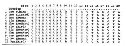
Part of the data matrix of aligned nucleotide sequences for the malaria parasite Plasmodium. Shown are the first 20 columns of the 11 × 221 matrix x of polytypic sites used in most of the analyses below. The final analysis of the last section also uses the data from 1399 monotypic sites.

Fig. 2 shows a phylogenetic tree constructed from x. The tree-building algorithm proceeds in two main steps: (i) an 11 × 11 distance matrix D̂ is constructed for the 11 species, measuring differences between the row vectors of x; and (ii) D̂ is converted into a tree by a connection algorithm that connects the closest two entries (species 9 and 10 here), reduces D̂ to a 10 × 10 matrix according to some merging rule, connects the two closest entries of the new D matrix, etc.

Figure 2.

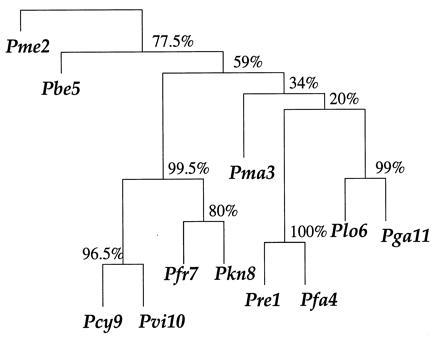
Phylogenetic tree based on the malaria data matrix; species are numbered as in Fig. 1. The numbers at the branches are confidence values based on Felsenstein’s bootstrap method. B = 200 bootstrap replications.

We can indicate the tree-building process schematically as

the hats indicating that we are dealing with estimated quantities. A deliberately simple choice of algorithms was made in constructing Fig. 2: D̂ was the matrix of the Euclidean distances between the rows of x, with (A, G, C, T) interpreted numerically as (1, 2, 5, 6), while the connection algorithm merged nodes by maximization. Other, better, tree-building algorithms are available, as mentioned later in the paper. Some of these, such as the maximum parsimony method, do not involve a distance matrix, and some use all of the sites, including the monotypical ones. The discussion here applies just as well to all such tree-building algorithms.

Felsenstein’s method proceeds as follows. A bootstrap data matrix x* is formed by randomly selecting 221 columns from the original matrix x with replacement. For example the first column of x* might be the 17th column of x, the second might be the 209th column of x, the third the 17th column of x, etc. Then the original tree-building algorithm is applied to x*, giving a bootstrap tree *,

This whole process is independently repeated some large number B times, B = 200 in Fig. 2, and the proportions of bootstrap trees agreeing with the original tree are calculated. “Agreeing” here refers to the topology of the tree and not to the length of its arms.

These proportions are the bootstrap confidence values. For example the 9-10 clade seen in Fig. 2 appeared in 193 of the 200 bootstrap trees, for an estimated confidence value of 0.965. Species 7-8-9-10 occurred as a clade in 199 of the 200 bootstrap trees, giving 0.995 confidence. (Not all of these 199 trees had the configuration shown in Fig. 2; some instead first having 8 joined to 9-10 and then 7 joined to 8-9-10, as well as other variations.)

Felsenstein’s method is, nearly, a standard application of the nonparametric bootstrap. The basic assumption, further discussed in the next section, is that the columns of the data matrix x are independent of each other and drawn from the same probability distribution. Of course, if this assumption is a bad one, then Felsenstein’s method goes wrong, but that is not the point of concern here nor in the references, and we will take the independence assumption as a given truth.

The bootstrap is more typically applied to statistics ^θ that estimate a parameter of interest θ, both ^θ and θ being single numbers. For example, ^θ could be the sample correlation coefficient between the first two malaria species, Pre and Pme, at the 221 sites, with (A, G, C, T) interpreted as (1, 2, 5, 6): ^θ = 0.616. How accurate is ^θ as an estimate of the true correlation θ? The nonparametric bootstrap answers such questions without making distributional assumptions.

Each bootstrap data set x* gives a bootstrap estimate ^θ*, in this case the sample correlation between the first two rows of x*. The central idea of the bootstrap is to use the observed distribution of the differences ^θ* − ^θ  to infer the unobservable distribution of ^θ − θ; in other words to learn about the accuracy of ^θ. In our example, the 200 bootstrap replications of ^θ* − ^θ were observed to have expectation 0.622 and standard deviation 0.052. The inference is that ^θ is nearly unbiased for estimating θ, with a standard error of about 0.052. We can also calculate bootstrap confidence intervals for θ. A well-developed theory supports the validity of these inferences [see Efron and Tibshirani (1)].

Felsenstein’s application of the bootstrap is nonstandard in one important way: the statistic , unlike the correlation coefficient, does not change smoothly as a function of the data set x. Rather, is constant within large regions of the x-space, and then changes discontinuously as certain boundaries are crossed. This behavior raises questions about the bootstrap inferences, questions that are investigated in the sections that follow.

A Model For The Bootstrap

The rationale underlying the bootstrap confidence values depends on a simple multinomial probability model. There are K = 4¹¹ − 4 possible column vectors for x, the number of vectors of length 11 based on a 4-letter alphabet, not counting the 4 monotypic ones. Call these vectors X₁, X₂, . . ., X_K, and suppose that each observed column of x is an independent selection from X₁, X₂, . . ., X_K, equaling X_k with probability π_k. This is the multinomial model for the generation of x.

Denote ˜π = (π₁, π₂,. . ., π_K), so the sum of ˜π’s coordinates is 1. The data matrix x can be characterized by the proportion of its n = 221 columns equalling each possible X_k, say

with ˜π̂ = (π̂₁, π̂₂, . . ., π̂_K). This is a very inefficient way to represent the data, since 4¹¹ − 4 is so much bigger than 221, but it is useful for understanding the bootstrap. Later we will see that only the vectors X_k that actually occur in x need be considered, at most n of them.

Almost always the distance matrix D̂ is a function of the observed proportions ˜π̂, so we can write the tree-building algorithm as

In a similar way the vector of true probabilities ˜π gives a true distance matrix and a true tree,

D would be the matrix with ijth element {∑_kπ_k(X_ki − X_kj)²}½ in our example, and TREE the tree obtained by applying the maximizing connection algorithm to D.

Fig. 3 is a schematic picture of the space of possible ˜π vectors, divided into regions ℛ₁, ℛ₂, . . .. The regions correspond to different possible trees, so if ∈ ℛ_j the jth possible tree results. We hope that = TREE, which is to say that ˜π and ˜π̂ lie in the same region, or at least that and TREE agree in their most important aspects.

Figure 3.

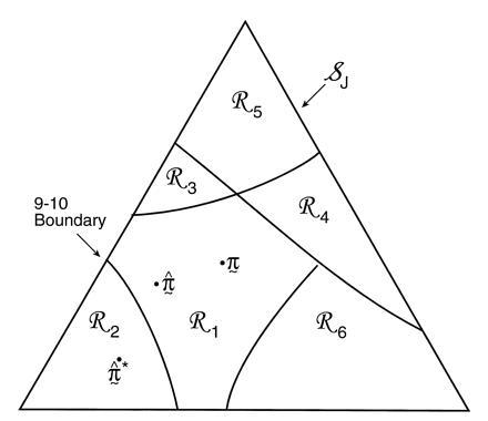
Schematic diagram of tree estimation; triangle represents the space of all possible ˜π vectors in the multinomial probability model; regions ℛ₁, ℛ₂. . . correspond to the different possible trees. In the case shown ˜π and ˜π̂ lie in the same region so TREE = , but ˜π̂* lies in a region where * does not have the 9-10 clade.

The bootstrap data matrix x* has proportions of columns say

* = (π̂₁^*, π̂₂^*, … . , π̂_K^*). We can indicate the bootstrap tree-building

The hypothetical example of Fig. 3 puts ˜π and ˜π̂ in the same region, so that the estimate exactly equals the true TREE. However ˜π̂* lies in a different region, with * not having the 9-10 clade. This actually happened in 7 out of the 200 bootstrap replications for Fig. 2.

What the critics of Felsenstein’s method call its bias is the fact that the probability * = TREE is usually less than the probability = TREE. In terms of Fig. 3, this means that ˜π̂* has less probability than ˜π̂ of lying in the same region as ˜π. Hillis and Bull (3) give specific simulation examples. The discussion below is intended to show that this property is not a bias, and that to a first order of approximation the bootstrap confidence values provide a correct assessment of ’s accuracy. A more valid criticism of Felsenstein’s method, discussed later, involves its relationship with the standard theory of statistical confidence levels based on hypothesis tests.

Returning to the correlation example of the previous section, it is not true that ^θ* − θ (as opposed to ^θ* − ^θ) has the same distribution as ^θ − θ, even approximately. In fact ^θ* − θ will have nearly twice the variance of ^θ − θ, the sum of the variances of ^θ around θ and of ^θ* around ^θ. Similarly in Fig. 3 the average distance from ˜π̂* to ˜π will be greater than the average distance from ˜π̂ to ˜π. This is the underlying reason for results like those of Hillis and Bull, that ˜π̂* has less probability than ˜π̂ of lying in the same region as ˜π. However, to make valid bootstrap inferences we need to use the observed differences between * and (not between * and TREE) to infer the differences between and TREE. Just how this can be done is discussed using a simplified model in the next two sections.

A Simpler Model

The meaning of the bootstrap confidence values can be more easily explained using a simple normal model rather than the multinomial model. This same tactic is used in Felsenstein and Kishino (4). Now we assume that the data x = (x₁, x₂) is a two dimensional normal vector with expectation vector μ = (μ₁, μ₂) and identity covariance matrix, written

In other words x₁ and x₂ are independent normal variates with expectations μ₁ and μ₂, and variances 1. The obvious estimate of μ is μ̂ = x, and we will use this notation in what follows. The μ-plane is partitioned into regions ℛ₁, ℛ₂, ℛ₃, . . . similarly to Fig. 3. We observe that μ̂ lies in one of these regions, say ℛ₁, and we wish to assign a confidence value to the event that μ itself lies in ℛ₁.

Two examples are illustrated in Fig. 4. In both of them x = μ̂ = (4.5,0) lies in ℛ₁, one of two possible regions. Case I has ℛ₂ = {μ : μ₁ ≤ 3}, a half-plane, while case II has ℛ₂ = {μ : ∥μ∥ ≤3}, a disk of radius 3.

Figure 4.

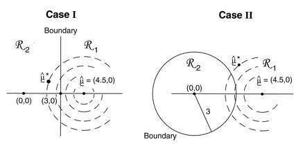
Two cases of the simple normal model; in both we observe μ̂ = (4.5, 0) ∈ ℛ₁, and wish to assign a confidence value to μ ∈ ℛ₁. Case I, ℛ₂ is the region {μ₁ ≤ 3}. Case II, ℛ₂ is the region {∥μ∥ < 3}. The dashed circles indicate bootstrap sampling μ̂* ∼ N₂(μ̂, I).

Bootstrap sampling in our simplified problem can be taken to be

This is a parametric version of the bootstrap, as in section 6.5 of Efron and Tibshirani (1), rather than the more familiar nonparametric bootstrap considered previously, but it provides the proper analogy with the multinomial model. The dashed circles in Fig. 4 indicate the bootstrap density of μ̂* = x*, centered at μ̂. Felsenstein’s confidence value is the bootstrap probability that μ̂* lies in ℛ₁, say

The notation Prob_μ̂ emphasizes that the bootstrap probability is computed with μ̂ fixed and only μ̂* random. The bivariate normal model of this section is simple enough to allow the α̃ values to be calculated theoretically, without doing simulations,

Notice that α̃_II is bigger than α̃_I because ℛ₁ is bigger in case II.

In our normal model, μ̂* − μ̂ has the same distribution as μ̂ − μ, both distributions being the standard bivariate normal N₂(0, I). The general idea of the bootstrap is to use the observable bootstrap distribution of μ̂* − μ̂ to say something about the unobservable distribution of the error μ̂ − μ. Notice, however, that the marginal distribution of μ̂* − μ has twice as much variance,

This generates the “bias” discussed previously, that μ̂* has less probability than μ̂ of being in the same region as μ. But this kind of interpretation of bootstrap results cannot give correct inferences. Newton (5) makes a similar point, as do Zharkikh and Li (6) and Felsenstein and Kishino (4).

We can use a Bayesian model to show that α̃ is a reasonable assessment of the probability that ℛ₁ contains μ. Suppose we believe apriori that μ could lie anywhere in the plane with equal probability. Then having observed μ̂, the aposteriori distribution of μ given μ̂ is N₂(μ̂, I), exactly the same as the bootstrap distribution of μ̂*. In other words, α̃ is the aposteriori probability of the event μ ∈ ℛ₁, if we begin with an “uninformative” prior density for μ.

Almost the same thing happens in the multinomial model. The bootstrap probability that * = is almost the same as the aposteriori probability that TREE = starting from an uninformative prior density on ˜π [see section 10.6 of Efron (7)]. The same statement holds for any part of the tree, for example the existence of the 9-10 clade in Fig. 2. There are reasons for being skeptical about the Bayesian argument, as discussed in the next section. However, the argument shows that Felsenstein’s bootstrap confidence values are at least reasonable and certainly cannot be universally biased downward.

Hypothesis-Testing Confidence Levels

Fig. 5 illustrates another more customary way of assigning a confidence level to the event μ ∈ ℛ₁. In both case I and case II, μ̂₀ = (3, 0) is the closest point to μ̂ on the boundary separating ℛ₁ from ℛ₂. We now bootstrap from μ̂₀ rather than from μ̂, obtaining bootstrap data vectors

[The double star notation is intended to avoid confusion with the previous bootstrap vectors x* ∼ N₂(μ̂, I).] The confidence level α̂ for the event μ ∈ ℛ₁ is the probability that the bootstrap vector μ̂** = x** lies closer than μ̂ to the boundary. This has a familiar interpretation: 1 − α̂ is the rejection level, one-sided, of the usual likelihood ratio test of the null hypothesis that μ does not lie in ℛ₁. Here we are computing α̂ numerically, rather than relying on an asymptotic χ² approximation. In a one-dimensional testing problem, 1 − α̂ would exactly equal the usual p value obtained from the test of the null hypothesis that the true parameter value lies in ℛ₂.

Figure 5.

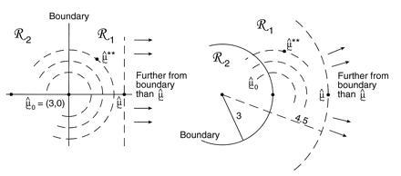
Confidence levels of the two cases in Fig. 4; μ̂₀ = (3, 0) is the closest point to μ̂ = (4.5, 0) on the boundary separating ℛ₁ from ℛ₂; bootstrap vector μ̂** ∼ N₂(μ̂₀, I). The confidence level α̂ is the probability that μ̂** is closer than μ̂ to the boundary.

Once again it is simple to compute the confidence level for our two cases, at least numerically,

In the first case α̂_I equals α̃_I, the Felsenstein bootstrap confidence value. However α̂_II = 0.914 is less than α̃_II = 0.949.

Why do the answers differ? Comparing Figs. 4 and 5, we see that, roughly speaking, the confidence value α̃ is a probabilistic measure of the distance from μ̂ to the boundary, while the confidence level α̂ measures distance from the boundary to μ̂. The two ways of measuring distance agree for the straight boundary, but not for the curved boundary of case II. Because the boundary curves away from μ̂, the confidence value α̃ is increased from the straight-line case. However the set of vectors further than μ̂ from the boundary curves toward μ̂₀, which decreases α̂. We would get the opposite results if the boundary between ℛ₁ and ℛ₂ curved in the other direction.

The confidence level α̂, rather than α̃, provides the more usual assessment of statistical belief. For example in case II let θ = ∥μ∥ be the length of the expectation vector μ. Then α̂ = 0.914 is the usual confidence level attained for the event {θ ≥ 3}, based on observing θ̂ = ∥μ̂∥ = 4.5. And {θ ≥ 3} is the same as the event {μ ∈ ℛ₁}.

Using the confidence value α̃ is equivalent to assuming a flat Bayesian prior for μ. It can be shown that using α̂ amounts, approximately, to assuming a different prior density for μ, one that depends on the shape of the boundary. In case II this prior is uniform on polar coordinates for μ, rather than uniform on the original rectangular coordinates [see Tibshirani (8)].

The Relationship Between the Two Measures of Confidence

There is a simple approximation formula for converting a Felsenstein confidence value α̃ to a hypothesis-testing confidence level α̂. This formula is conveniently expressed in terms of the cumulative distribution function Φ(z) of a standard one-dimensional normal variate, and its inverse function Φ⁻¹: Φ(1.645) = 0.95, Φ⁻¹(0.95) = 1.645, etc. We define the “z values” corresponding to α̃ and α̂,

In case II, z̃ = Φ⁻¹(0.949) = 1.64 and ẑ = Φ⁻¹(0.914) = 1.37.

Now let μ̂** ∼ N₂(μ̂₀,I) as in Fig. 5, and define

For case I it is easy to see that z₀ = Φ⁻¹(0.50) = 0. For case II, standard calculations show that z₀ = Φ⁻¹(0.567) = 0.17.

In normal problems of the sort shown in Figs. 4 and 5 we can approximate ẑ in terms of z̃ and z₀:

1

Formula 1 is developed in Efron (9), where it is shown to have “second order accuracy.” This means that in repeated sampling situations [where we observe independent data vectors x₁, x₂, . . . , x_n ∼ N₂(μ, I) and estimate μ by μ̂ = ∑_iⁿ= x_i/n] z₀ is of order 1/, and formula 1 estimates ẑ with an error of order only 1/n.

Second-order accuracy is a large sample property, but it usually indicates good performance in actual problems. For case I, Eq. 1 correctly predicts ẑ = z̃, both equalling Φ⁻¹(0.933) = 1.50. For case II the prediction is ẑ = 1.64 − 0.34 = 1.30, compared with the actual value ẑ = 1.37.

Formula 1 allows us to compute the confidence level α̂ for the event {μ ∈ ℛ₁} solely in terms of bootstrap calculations, no matter how complicated the boundary may be. A first level of bootstrap replications with μ̂* ∼ N₂(μ̂, I) gives bootstrap data vectors μ̂*(1), μ̂*(2), . . ., μ̂*(B), from which we calculate

A second level of bootstrap replications with μ̂** ∼ N₂(μ̂₀,I), giving say μ̂**(1), μ̂**(2), . . ., μ̂**(B₂), allows us to calculate

Then formula 1 gives ẑ = z̃ − 2z₀.

As few as B = 100, or even 50, replications μ̂* are enough to provide a rough but useful estimate of the confidence value α̃. However, because the difference between z̃ = Φ⁻¹(α̃) and ẑ = Φ⁻¹(α̂) is relatively small, considerably larger bootstrap samples are necessary to make formula 1 worthwhile. The calculations in section 9 of Efron (9) suggest both B and B₂ must be on the order of at least 1000. This point did not arise in cases I and II where we were able to do the calculations by direct numerical integration, but it is important in the kind of complicated tree-construction problems we are actually considering.

We now return to the problem of trees, as seen in Fig. 2. The version of formula 1 that applies to the multinomial model of Fig. 3 is

2

Here “a” is the acceleration constant introduced in ref. 9. It is quite a bit easier to calculate than z₀, as shown in the next section. Formula 2 is based on the bootstrap confidence intervals called “BC_a” in ref. 9.

If we tried to draw Fig. 3 accurately we would find that the multi-dimensional boundaries were hopelessly complicated. Nevertheless, formula 2 allows us to obtain a good approximation to the hypothesis-testing confidence level α̂ = Φ(ẑ) solely in terms of bootstrap computations. How to do so is illustrated in the next section.

An Example Concerning the Malaria Data

Fig. 2 shows an estimated confidence value of

for the existence of the 9-10 clade on the malaria evolutionary tree. This value was based on B = 200 bootstrap replications, but (with some luck) it agrees very closely with the value α̃ = 0.962 obtained from B = 2000 replications. How does α̃ compare with α̂, the hypothesis-testing confidence level for the 9-10 clade? We will show that

(or α̂ = 0.938 if we begin with α̃ = 0.962 instead of 0.965). To put it another way, our nonconfidence in the 9-10 clade goes from 1 − α̃ = 0.035 to 1 − α̂ = 0.058, a substantial change.

We will describe, briefly, the computational steps necessary to compute α̂. To do so we need notation for multinomial sampling. Let P = (P₁, P₂, . . ., P_n) indicate a probability vector on n = 221 components, so the entries of the vector P are nonnegative numbers summing to 1. The notation

will indicate that P* = (P₁^*, P₂^*, … , P_n^*) is the vector of proportions obtained in a multinomial sample of size n from P. In other words we independently draw integers I₁^*, I₂^*, . . , I_n^* from {1, 2, . . , n} with probability P_k on k, and record the proportions P_k^* = #{I_i^* = k}/n. This is the kind of multinomial sampling pictured in Fig. 3, expressed more efficiently in terms of n = 221 coordinates instead of K = 4¹¹ − 4.

Each vector P* is associated with a data matrix x* that has proportion P_k^* of its columns equal to the kth column of the original data matrix x. Then P* determines a distance matrix and a tree according to the original tree-building algorithm,

The “central” vector

corresponds to the original data matrix x and the original tree . Notice that taking P* ∼Mult(P^(cent)) amounts to doing ordinary bootstrap sampling, since then x* has its columns chosen independently and with equal probability from the columns of x.

Resampling from P^(cent) means that each of the 221 columns is equally likely, but this is not the same as all possible 11 vectors being equally likely. There were only 149 distinct 11 vectors among the columns of x, and these are the only ones that can appear in x*. The vector TTTTCTTTTTT appeared seven times among the columns of x, so it shows up seven times as frequently in the columns of x*, compared with ATAAAAAAAAA which appeared only once in x.

Here are the steps in the computation of α̂.

Step 1. B = 2000 first-level bootstrap vectors P*(1), P*(2), . . ., P*(B) were obtained as independent multinomials P* ∼ Mult(P^(cent)). Some 1923 of the corresponding bootstrap trees had the 9-10 clade, giving the estimate α̃ = 0.962 = 1923/2000.

Step 2. The first 200 of these included seven cases without the 9-10 clade. Call the seven P* vectors P⁽¹⁾, P⁽²⁾, . . ., P⁽⁷⁾. For each of them, a value of w between 0 and 1 was found such that the vector

was right on the 9-10 boundary. The vectors p^(j) play the role of μ̂₀ in Fig. 5.

Finding w is easy using a one-dimensional binary search program, as on page 90 of ref. 10. At each step of the search it is only necessary to check whether or not the current value of wP^(j) + (1 − w)P^(cent) gives a tree having the 9-10 clade. Twelve steps of the binary search, the number used here, locates the boundary value of w within 1/2¹². The vectors p^(j) play the role of μ̂₀ in Fig. 5.

Step 3. For each of the boundary vectors p^(j) we generated B₂ = 400 second-level bootstrap vectors

computed the corresponding tree, and counted the number of trees having the 9-10 clade. The numbers were as follows for the seven cases:

From the total we calculated an estimate of the correction term z₀ in formula 2,

Binomial calculations indicate that z₀ = 0.0995 has a standard error of about 0.02 due to the bootstrap sampling (that is, due to taking 2800 instead of all possible bootstrap replications), so 2800 is not lavishly excessive. Notice that we could have started with the 77 out of the 2000 P* vectors not having the 9-10 clade, rather than the 7 out of the first 200, and taken B₂ = 40 for each p^(j), giving about the same total second-level sample.

Step 4. The acceleration constant “a” appearing in formula 2 depends on the direction from P^(cent) to the boundary, as explained in section 8 of ref. 9. For a given direction vector U,

Taking U = p^(j) − P^(cent) for each of the seven cases gave

Step 5. Finally we applied formula 2 with z̃ = Φ⁻¹(0.962) = 1.77, z₀ = 0.0995, and a = 0.0129, to get ẑ = 1.54, or α̂ = Φ(ẑ) = 0.938. If we begin with z̃ = Φ⁻¹(0.965) then α̂ = 0.942.

Notice that in this example we could say that Felsenstein’s bootstrap confidence value α̃ was biased upward, not downward, at least compared with the hypothesis-testing level α̂. This happened because z₀ was positive, indicating that the 9-10 boundary was curving away from P^(cent), just as in case 2 of Fig. 5. The opposite can also occur, and in fact did for other clades. For example the clade at the top of Fig. 2 that includes all of the species except lizard (species 2) had α̃ = 0.775 compared with α̂ = 0.875.

We carried out these same calculations using the more efficient tree-building algorithm employed in Escalante and Ayala (11); that is we used Felsenstein’s phylip package (12) on the complete RNA sequences, neighbor-joining trees based on Kimura’s (13) two-parameter distances.

In order to vary our problem slightly, we looked at the clade 7-8 (Pfr-Pkn), which is more questionable than the 9-10 clade. The tree produced from the original set is:

Step 1. B = 2000 first-level bootstrap vectors. Some 1218 of the corresponding bootstrap trees had the 7-8 clade, giving the estimate α̃ = 0.609 = 1218/2000.

Step 2. We took, as before, seven cases without the 7-8 clade, and for each one found a multinomial vector near the 7-8 boundary.

Step 3. For each of the boundary vectors p^(j) we generated B₂ = 400 second-level bootstrap vectors

computed the corresponding tree, and counted the number of trees having the 7-8 clade. The numbers were as follows for the seven cases:

From the total we calculated an estimate of the correction term z₀ in formula 2,

Step 4. The acceleration constant “a” appearing in formula 2 was computed as before giving:

Step 5. Finally we applied formula 2 with z̃ = Φ⁻¹(0.609) = 0.277 to get ẑ = 0.417, or α̂ = Φ(ẑ) = 0.662. In this case α̂ is bigger than α̃, reflecting the fact that the 7-8 boundary curves toward the central point, at least in a global sense.

Computing α̂ is about 20 times as much work as α̃, but it is work for the computer and not for the investigator. Once the tree-building algorithm is available, all of the computations require no more than applying this algorithm to resampled versions of the original data set.

Discussion and Summary

The discussion in this paper, which has gone lightly over many technical details of statistical inference, makes the following main points about the bootstrapping of phylogenetic trees.

(i) The confidence values α̃ obtained by Felsenstein’s bootstrap method are not biased systematically downward.

(ii) In a Bayesian sense, the α̃ can be thought of as reasonable assessments of error for the estimated tree.

(iii) More familiar non-Bayesian confidence levels α̂ can also be defined. Typically α̂ and α̃ will converge as the number n of independent sites grows large, at rate 1/.

(iv) The α̂ can be estimated by a two-level bootstrap algorithm.

(v) As few as 100 or even 50 bootstrap replications can give useful estimates of α̃, while α̂ estimates require at least 2000 total replications. None of the computations requires more than applying the original tree-building algorithm to resampled data sets.

References

- 1.Efron B, Tibshirani R. An Introduction to the Bootstrap. London: Chapman & Hall; 1993. [Google Scholar]
- 2.Felsenstein J. Evolution. 1985;39:783–791. doi: 10.1111/j.1558-5646.1985.tb00420.x. [DOI] [PubMed] [Google Scholar]
- 3.Hillis D, Bull J. Syst Biol. 1993;42:182–192. [Google Scholar]
- 4.Felsenstein J, Kishino H. Syst Biol. 1993;42:193–200. [Google Scholar]
- 5.Newton M A. Biometrika. 1996;83:315–328. [Google Scholar]
- 6.Zharkikh A, Li W H. Mol Biol Evol. 1992;9:1119–1147. doi: 10.1093/oxfordjournals.molbev.a040782. [DOI] [PubMed] [Google Scholar]
- 7.Efron, B. (1982) SIAM CBMS-NSF Monogr. 38.
- 8.Tibshirani R J. Biometrika. 1989;76:604–608. [Google Scholar]
- 9.Efron B. J Am Stat Assoc. 1987;82:171–185. [Google Scholar]
- 10.Press W, Flannery B, Teukolsky S, Vetterling W. Numerical Recipes. New York: Cambridge Univ. Press; 1987. [Google Scholar]
- 11.Escalante A, Ayala F. Proc Natl Acad Sci USA. 1995;92:5793–5797. doi: 10.1073/pnas.92.13.5793. [DOI] [PMC free article] [PubMed] [Google Scholar]
- 12.Felsenstein, J. (1993) phylip (Univ. of Washington, Seattle).
- 13.Kimura M. J Mol Evol. 1980;16:111–120. doi: 10.1007/BF01731581. [DOI] [PubMed] [Google Scholar]
- 14.Escalante A, Ayala F. Proc Natl Acad Sci USA. 1994;91:11371–11377. [Google Scholar]