Spatial Frequency Maps in Cat Visual Cortex

Abstract

Neurons in the primary visual cortex (V1) respond preferentially to stimuli with distinct orientations and spatial frequencies. Although the organization of orientation selectivity has been thoroughly described, the arrangement of spatial frequency (SF) preference in V1 is controversial. Several layouts have been suggested, including laminar, columnar, clustered, pinwheel, and binary (high and low SF domains). We have reexamined the cortical organization of SF preference by imaging intrinsic cortical signals induced by stimuli of various orientations and SFs. SF preference maps, produced from optimally oriented stimuli, were verified using targeted microelectrode recordings. We found that a wide range of SFs is represented independently and mostly continuously within V1. Domains with SF preferences at the extremes of the SF continuum were separated by no more than ¾ mm (conforming to the hypercolumn description of cortical organization) and were often found at pinwheel center singularities in the cortical map of orientation preference. The organization of cortical maps permits nearly all combinations of orientation and SF preference to be represented in V1, and the overall arrangement of SF preference in V1 suggests that SF-specific adaptation effects, found in psychophysical experiments, may be explained by local interactions within a given SF domain. By reanalyzing our data using a different definition of SF preference than is used in electrophysiological and psychophysical studies, we can reproduce the different SF organizations suggested by earlier studies.

The columnar arrangement of striate cortex is arguably its hallmark and, as a result, much of the work aimed at understanding the mechanisms of vision has focused on characterizing visual cortical columns (for review, see LeVay and Nelson, 1991). Although the maps of both ocular dominance (LeVay et al., 1978; Anderson et al., 1988; Bonhoeffer et al., 1995) and orientation preference (Hubel and Wiesel, 1962; Thompson et al., 1983;Bonhoeffer and Grinvald, 1991) of the cat have been well characterized in the primary visual cortex (V1), the cortical organization of spatial frequency (SF) preference is less clear. Past experiments have described the organization of SF preference in cats as laminar (Maffei and Fiorentini, 1977), clustered (Tolhurst and Thompson, 1982), or columnar (Tootell et al., 1981; Silverman, 1984; Bonhoeffer et al., 1995). Together, these and other studies (Movshon et al., 1978a;Tolhurst and Thompson, 1981) suggest that, like ocular dominance, the SF preference of cortical cells varies both tangentially across the cortical surface and radially through the cortical laminae. The techniques classically used to assess cortical organization (single-unit recording and metabolic staining) are inherently limited, however, and have not provided a definitive characterization of the structure of the cortical SF map. In addition, SF preference is less similar among neighboring cortical neurons than are other receptive field properties, such as orientation preference (De Angelis et al., 1999), making a characterization of the cortical SF map based on single-unit responses difficult.

Optical imaging of intrinsic signals permits the measurement of cortical responses over a large area of cortex (for review, seeBonhoeffer and Grinvald, 1996). Two recent sets of experiments have used intrinsic signal imaging to characterize the tangential organization of SF preference in cat primary visual cortex. These experiments, however, support opposing models. The first set of experiments (Bonhoeffer et al., 1995; Hubener et al., 1997; Shoham et al., 1997) supports a model of cortical SF representation based on the segregation of the X and Y pathways into cortical domains (for review, see Sherman, 1985). Compared with Y cells, X cells have smaller receptive fields and respond preferentially to higher spatial, and lower temporal, frequencies. These features and others have led researchers to conclude that, whereas Y cells mediate the analysis of basic visual forms, X cells refine this process through the addition of higher spatial resolution (for review, see Stone et al., 1979; Sherman, 1985). Intrinsic signal images of primary visual cortex obtained while stimulating the visual system with a variety of spatial frequencies were interpreted as showing only regions of “high” and “low” SF preference (Bonhoeffer et al., 1995; Hubener et al., 1997; Shoham et al., 1997). The presence of high and low SF preferences in separate cortical domains is consistent with the proposed cortical segregation of X and Y inputs from the thalamus (Shoham et al., 1997).

A second set of imaging experiments (Everson et al., 1998) supports a model in which the primary visual cortex contains multiple domains representing many different spatial frequencies. Maps of SF preference made using principal component analysis of intrinsic signals appeared to be organized in “pinwheels” (analogous to orientation pinwheels) (Bonhoeffer and Grinvald, 1991), around which all SFs are represented. Human psychophysical experiments also suggest that there is a continuous distribution of SF preference in the visual cortex, although they do not provide evidence for a particular organization. Studies of SF-specific adaptation (Blakemore and Campbell, 1969), as well as observations made during SF discrimination tasks (Watson and Robson, 1981), provide compelling evidence that the visual cortex has multiple processing channels, each tuned to one of many different SF ranges (Graham and Nachmias, 1971; Sachs et al., 1971; Watson, 1982). In accord with this, single-unit recordings in cat V1 demonstrate a wide range of SF preferences and tuning bandwidths at single retinotopic loci (Movshon et al., 1978b; Tolhurst and Thompson, 1981;Robson et al., 1988). These data provide convergent evidence that SF preference in the visual cortex is unlikely to result simply from differences between X and Y cell response characteristics.

To identify the model that best describes the organization of SF preference in the primary visual cortex of the cat, we have used a combination of intrinsic signal optical imaging and multi-unit microelectrode recordings to assess SF preference in V1. We found that a wide range of SF preferences is mapped onto the visual cortex. This representation was mostly continuous, with SF generally changing gradually and progressively in the tangential plane but with occasional linear discontinuities. Tuning curves constructed from optical maps, and confirmed by microelectrode recording, demonstrated that the arrangement of SF preference is derived from a collection of many domains, each of which is selective for a narrow range of SF.

Parts of this work have been published previously in abstract form (Trepel et al., 1999).

MATERIALS AND METHODS

Optical imaging of intrinsic signals was used to examine the layout of SF preference in cortical areas 17 and 18 of seven cats between 7 and 16 weeks of age. Previous work has shown that contrast sensitivity reaches adult levels at ∼6 weeks of age (Derrington and Fuchs, 1981). All animals were bred and reared in the University of California at San Francisco (UCSF) animal care facility under an 18/6 hr light/dark cycle. All experimental procedures were approved by the UCSF Committee on Animal Research.

Surgical preparation. Animals were initially anesthetized with the inhaled anesthetic isoflurane (3–4% in O₂) and, after implantation with a femoral catheter, were switched to a short-lived barbiturate (thiopental). Atropine (0.25–0.4 mg) and dexamethasone (0.4–0.8 mg) were injected subcutaneously to reduce tracheal secretions and minimize the stress response, respectively. A tracheotomy was performed, and a long-lasting barbiturate (sodium pentobarbital) was substituted for thiopental. To assess the anesthetic state of an animal, we continuously monitored its core temperature, electrocardiogram, expired CO₂, and peak airway pressure. A feedback-regulated heating pad maintained core body temperature at 37.5°C. Pentobarbital was administered as needed to keep the animal at a surgical plane of anesthesia, determined by the animal's heart rate and peak expired CO₂.

The animal was placed in a stereotaxic apparatus, and 1% atropine sulfate and 10% phenylephrine hydrochloride were applied to the eyes. To focus the eyes on the stimulus monitor, contact lenses of the appropriate strength were fitted with the aid of a retinoscope or by maximizing visual acuity for each eye as measured by visually evoked potentials (two cats) (Tang and Norcia, 1993). A craniotomy was made over the lateral gyrus of both hemispheres. Neuromuscular blockade was then induced by continuous infusion of gallamine triethiodide (10 mg · kg⁻¹ · hr⁻¹) mixed in 2.5% dextrose in lactated Ringer's solution (total volume of fluid infused, 5–10 m1 · kg⁻¹ · hr⁻¹), and the animal was ventilated for the duration of the experiment. The dura mater was reflected, and low-melting point agarose (3% in saline) and a glass coverslip were placed over the exposed cortex. The optic disks were plotted, and artificial pupils (3 mm diameter) were placed in front of the area centrales.

Optical imaging of intrinsic signals. All imaging of V1 was done on the flat part of V1 on the dorsal surface of the lateral gyrus, corresponding to the area in visual field within 10° of the vertical meridian and between the horizontal meridian and 10° into the lower field. Optical images of cortical intrinsic signal were obtained using the ORA-2000 Optical Recording Acquisition and Analysis System (Optical Imaging, Inc., Germantown, NY). Using different tandem lens configurations (Nikon Inc., Melville, NY), both “low-resolution” (50 × 50 mm lenses, 6.0 × 8.0 mm image area) and “high-resolution” (135 × 50 mm lenses, 2.4 × 3.2 mm image area) images could be acquired. The surface vascular pattern or intrinsic signal images were visualized with illumination wavelengths set by a green (546 ± 10 nm) or red (610 ± 10 nm) interference filter, respectively. After acquisition of a surface image, the camera was focused 400–500 μm below the pial surface, an additional red filter was interposed between the brain and slow-scan CCD camera, and intrinsic signal images were acquired. Images were stored as 192 × 144 pixels after binning the 384 × 288 camera pixels by 2.

Visual stimulus patterns were varied according to the stimulus parameter being mapped. Full-field sine and square wave grating stimuli were generated by a VSG 2/3 board (Cambridge Research Systems, Rochester, UK) controlled by custom software. Shutters for the light source, camera, and eyes were controlled by the stimulus and acquisition computers. A typical experiment began with a mapping of orientation and ocular dominance using drifting square wave gratings with a fundamental SF of 0.2 cycles (c) per degree and a temporal frequency of 2.0 c/sec. Stimuli were presented in pseudorandom order separately to the two eyes at eight orientations separated by 22.5°. Gratings reversed their direction of motion every 2 sec and were interspersed with four identical blank screen conditions (both eyes viewing a gray screen). There were therefore a total of 20 stimulus conditions for the gratings plus the blanks. We measured the degree to which both eyes could activate the cortex using the optical contralateral bias index described by Issa et al. (1999). For all high-resolution fields, the mean optical contralateral bias index was 0.50 ± 0.04 (range, 0.43–0.55), meaning that on average the two eyes were equally effective in driving cells in the field.

Spatial frequency mapping required a much larger number of stimulus conditions. A typical experiment involved the binocular presentation of sine wave gratings of eight orientations at six to eight spatial frequencies ranging between 0.1 and 1.84 c/°. Ideally, each mapping run would have randomly interleaved all stimulus conditions, but because the large number of stimulus combinations exceeded the capacity of the optical imaging software, stimulus conditions were distributed among either two or four sets that were run sequentially. Each stimulus set included a wide range of spatial frequencies and orientations and was designed to provide a coarse map on its own before combination with data from the other sets. In addition to the oriented gratings, each stimulus set included five blank stimuli and one grating stimulus that was common to all the stimulus sets. A map from eight orientations and eight spatial frequencies was therefore constructed from four stimulus sets, each of which consisted of 22 conditions: four orientations times four spatial frequencies plus five blanks plus a common condition. Responses to four of the blank stimuli were used to construct an average “blank” image, and the response to the fifth blank stimulus was used to determine the noise level in the data set. The visual stimulus that was common to all the stimulus sets was used to verify the stability of the responses across the sets before combining responses from different sets into a single SF map. If the mean intensity in the active areas of the images produced in response to the common stimulus differed among the stimulus sets by >1 SD, the data set was discarded.

At the beginning of each trial, a stationary grating was presented for 5 sec. The grating then began to drift at a temporal frequency of 2 Hz, and acquisition of 20–25 frames of 250–300 msec duration each began. Within a stimulus set, each of the stimuli was presented 16 times in a different random order, and the different stimulus sets of an experiment were interleaved. Two to four runs of each set were analyzed for each experiment. Images were analyzed using commercial (ORA-2000) and custom software written in the Interactive Data Language (Research Systems, Boulder, CO).

Raw images were normalized by the average of images acquired during the blank screen conditions (“blank normalization”) (Crair et al., 1997b). This form of normalization makes no assumptions about the structure of the functional maps. Because it takes 3–6 min to acquire a single set of images, there can be small difference in baseline intensity among the different stimulus conditions. To eliminate these differences, normalized single-condition response maps were high-pass filtered (2.35 × 2.35 mm uniform kernel). These maps were then smoothed (50 × 50 μm uniform kernel) before being combined for the calculation of SF maps. No further smoothing was done on the derived maps.

Calculation of spatial frequency maps. Three different types of SF map were constructed to graphically represent SF preferences over a cortical area. In the first type, the “SF map” (see Fig.5), the preferred SF of a pixel was defined as the SF of the single stimulus condition that produced the strongest response at that pixel among all of the unique combinations of orientation and SF. The color of each pixel was determined by its preferred SF, and lightness and saturation were held constant: red represents a low SF, orange through yellow, green, and blue represent increasing intermediate frequencies, and purple represents the highest SF. In the second type of map, the “SF response map”, the preferred SF of a pixel was displayed as above, but the lightness of the pixel was set in proportion to the magnitude of the response to the best stimulus. In SF response maps (see Figs. 2, 3), pixels that are dark have a very small best response. In the third type of map, the “interpolated SF map” (Fig.5E), the preferred SF of each pixel was determined by interpolating a peak SF from the tuning curve of a single pixel at the optimal stimulus orientation. Therefore, any continuity of SF preference observed in interpolated SF maps cannot be an artifact of the technique used to construct the map but must be a function of the genuine cortical representation of SF preference. The first and third types of SF maps are analogous to the “angle map” used for the display of orientation columns, whereas the second is analogous to the “polar map” (Bonhoeffer and Grinvald, 1996).

Fig. 5.

SF maps show linear discontinuities.A, An SF map produced in response to the eight SF stimuli marked on the color bar below thepanel; the SF scale shown on this color bar is shared with E. Orientation pinwheel centers are marked with asterisks inA–D. The area marked by a square is shown rotated in Figure 3. B–D, The SF map inB was produced in response to six SFs (0.2, 0.35, 0.5, 0.7, 0.95, and 1.2), marked with short lines on thesecond color bar. The SF maps in C andD were produced in response to the seven SFs marked on the second color bar. E, The interpolated SF map constructed from the same data used to make the SF map inA. F, Spatial frequency profile along the transect marked by the black line in Eand H. SF preference varies smoothly over this region.G, Spatial frequency profile along the transect marked by the white line in E andH. SF preference varies continuously over the initial segment of this transect but shifts at a fracture in the SF map.H, Spatial gradient of SF preference. Pixels at which SF preference varies rapidly are shown in red. Areas in which the spatial gradient is small are shown inblue.

Fig. 2.

A high-resolution spatial frequency map.A, A single-orientation SF map. Grayscale images are single-condition images showing the cortical response to single sinusoidal grating stimuli, each with an orientation of 45°, and the SF indicated in the panel. Dark regions in these images are active; all six images were scaled to the same absolute range of intrinsic signal intensities. Themiddle panel was constructed by color-coding each pixel according to the SF of the stimulus condition that most effectively drove the neurons at that pixel position. The brightnessof a pixel corresponds to the response strength of the pixel. Spatial frequency tuning curves for the three points marked on the single-orientation SF map are shown in the middle panelin the bottom row. The maximum response level is similar for the three tuning curves, although the points prefer very different spatial frequencies. Absolute response is shown as 10,000 times the difference between the optical signal produced in response to a stimulus and the signal produced in response to a blank screen.B, An all-orientation SF map. The eight panels surrounding the middle panel are the single-orientation SF maps constructed from the orientation shown on thepanel and the spatial frequencies shown inA. The middle panel was constructed by color-coding each pixel according to the SF of the stimulus condition that most effectively drove the neurons at that pixel. Orientation pinwheel centers are marked with asterisks.Color–lightness code for SF and response strength are as shown in A, except that maximum response for themiddle panel is 4.9 × 10⁻⁴. Maximum responses for eight surrounding panels vary from 4.0 to 4.9 × 10⁻⁴.

Fig. 3.

Multi-unit recordings validate spatial frequency maps. A, Microelectrode penetrations were targeted to specific SF domains in area 17. Microelectrode penetrations were made at the locations marked by black circles on the SF response map. In the optical and electrophysiological tuning curves, relative activity is plotted as a function of SF (line graph) and orientation (polar plot); for each tuning curve, the maximum response was set to a value of 1, and the minimum response was set to 0. Note that the penetrations shown are in “intermediate” SF domains (between 0.3 and 0.8 c/°). Orientation pinwheel centers are marked with asterisks. B, Preferred SF derived from optical maps plotted against preferred SF measured from unit recording. To show each data point, points that overly each other have been plotted adjacent to each other. A linear fit had a correlation coefficient r = 0.86 for 19 cells. The mean difference in orientation preference between optical and electrophysiological measurements was 4.2 ± 3.3° (mean ± SD). Scales are linear.

Because the range of potential SF preference is unbounded, it is possible that none of our stimulus conditions activated certain cortical regions. To prevent these regions from contributing to measurements of the SF map, pixels that had a best response near the noise level were not considered in generating tuning curves of SF preference (see Figs. 4, 7). The noise level was set at a multiple of the SD (ς) of the pixel intensities in a blank-normalized blank image: a single-condition image produced by stimulating with a mean-luminance blank screen. Unless otherwise noted, the noise level was set at 2ς. Because decreased reflectivity (i.e., a darker image) corresponds to increased activity, only pixels with best response values darker than 1.0 − noise level were considered to have stimulus-dependent activity.

Fig. 4.

Intermediate SF domains are independent of neighboring high and low SF domains. A, Average tuning curves at each SF peak for the SF map shown in Figure 2. Average tuning curves were constructed after first normalizing the response at each pixel such that 1 represents the maximum response of a pixel, and 0 represents the theoretical response of the cortex to a blank image. Tuning curves from all pixels that had the same peak SF preference and those whose peak response exceeded the 2ς noise level were averaged to give the tuning curves shown. The abscissa is a logarithmic axis. B, Hypothetical SF tuning curves, constructed from the linear summation of high and low SF domains, do not match the observed SF tuning curves. The hypothetical tuning curves were constructed by adding together weighted tuning curves from high and low SF domains:

$$\text{tuning curve} (f,SF)={TC}_{0.2}(SF)·f+{TC}_{0.95}(SF)·(1-f).$$

The weighting factor, f, varied from 0 to 1; each curve has a different value of f. TC_0.2was the tuning curve measured for pixels with a best response at 0.2 c/° (red curve in A), and TC_0.95 was the tuning curve measured for pixels with a best response of 0.95 c/° (purple curve inA).

Fig. 7.

The effect of stimulus orientation on spatial frequency preference. A, Average SF tuning curves for all pixels that respond most strongly to gratings with an SF of 0.2 c/°. Each tuning curve is constructed at a different stimulus orientation. The tuning curve labeled 0 is constructed from responses at preferred orientation of the pixels. The curves labeled 22 and 45 were constructed from responses of these same pixels to gratings presented at 22 or 45° from the preferred orientation. For each point in a tuning curve, only genuine responses were considered, using pixels whose response exceeded a 4ς noise level. B, Average SF tuning curves for all pixels that respond most strongly to gratings with an SF of 0.5 c/°. Tuning curves are labeled as in A. C, Average SF tuning curves for all pixels that respond most strongly to gratings with an SF of 0.95 c/°. Tuning curves are labeled as inA. D, Average preferred SF as a function of stimulus orientation. Spatial frequency preference was calculated for each pixel at each stimulus orientation. Each lineon the graph plots data from the pixels that preferred a given SF at their optimal orientation. The average SF preference was then calculated from the same pixels (in which their response exceeded the threshold described in A) for each stimulus orientation. The top profile, for example, was compiled from pixels that prefer 1.2 c/° at their optimal orientation (orientation difference of 0). At off-peak orientations, the preferred SF for these pixels was lower than that at the optimal orientation. Thetop and bottom lines aredashed to emphasize that their downward and upward profiles are obligate; they already have an extreme SF preference at the preferred orientation, and averaging any noise at off-peak orientations will produce a less extreme apparent SF preference. A 4ς noise level was used to minimize this effect. Note that preferred SF decreases as the orientation changes from the optimal for the four highest SFs studied.

Electrophysiology. To confirm that the optically imaged SF maps corresponded to the neuronal SF selectivity, we made targeted multi-unit recordings using electrolytically sharpened, resin-coated tungsten microelectrodes (1–3 MΩ). Unit responses were thresholded with a window discriminator to separate spike activity from electrical noise. A computer-based system running custom software presented randomly ordered gratings of different orientations and measured the spike rates of the cells. Once orientation preference was determined, subsequent stimuli consisted of pseudorandomly ordered gratings spanning a range of spatial frequencies presented at the preferred orientation. Blank-screen stimuli were presented interleaved with grating stimuli to provide a measure of spontaneous activity. Electrolytic lesions (4 sec, 4 μA) were made at the beginning and end of a penetration.

Multi-unit recordings were excluded from analysis if one of the following criteria were met: (1) the difference in orientation preference measured electrophysiologically and optically was greater than 11.25° (half the measurement interval); (2) the recording site was not in a superficial layer; or (3) the multi-unit SF tuning curve had multiple peaks. An area of 0.12 mm²(1.6% of the imaged area) around the targeted site was searched for the best match to the electrophysiologically measured orientation preference. In penetrations for which electrode tracks could not be reconstructed, only sites in the first 400 μm of a penetration were included.

At the end of a recording session, the animal was given a lethal dose of pentobarbital and transcardially perfused with 0.1 mphosphate buffer, followed by 10% paraformaldehyde. After post-fixing and cryoprotecting for at least 1 d in 10% paraformaldehyde–20% sucrose, the visual cortex was sectioned on a freezing microtome. Sections were Nissl stained, and electrode tracks and recording positions were reconstructed from camera lucida drawings.

RESULTS

We have defined the SF preference of a small region of cortex corresponding to a pixel in our maps as the SF of the single stimulus that best activated the pixel, among all the combinations of orientation and SF presented. The maps of SF preference constructed using this definition are very different from previously published maps (Hubener et al., 1997; Shoham et al., 1997; Everson et al., 1998).

Gross structure of the SF map

We used low-resolution images of cortical intrinsic signals to study the gross structure of the map of SF preference. The map shown in Figure 1 is consistent with the known layout of SF across the cat's lateral gyrus (Movshon et al., 1978b;Bonhoeffer et al., 1995). Area 18, occupying an anterior and lateral portion of the cat's lateral gyrus, was well stimulated by the two lowest spatial frequencies presented (0.1 and 0.16 c/°). Area 17, alternatively, was activated by gratings of higher spatial frequency. The difference in SF preference between areas 17 and 18 can be quantified by comparing the cumulative distributions of their SF preferences (Fig. 1). For pixels in area 17, the median preferred SF was 0.53 c/°. As expected, this was more than double the median preferred SF of area 18 (0.18 c/°).

Fig. 1.

The area 17/18 border is revealed by SF sensitivity. Top row, Polar orientation maps constructed from responses to eight differently oriented sine wave gratings at the specified SF. Hue represents orientation preference, andcolor lightness represents degree of tuning. For low SFs, area 17 is dark, indicating weak or poorly tuned responses to oriented gratings, but area 18 is active and well tuned. For intermediate SFs (0.43 and 0.70 c/°) both areas 17 and 18 are active and well tuned. At higher SFs, a pattern complementary to that seen at low SFs develops, with area 17 active and area 18 inactive. The polar map from stimuli at 3.0 c/° is not shown because there was no stimulus-dependent response. Bottom row, The left panel shows the vascular pattern in the region of cortex imaged. The lateral (Lat) and posterior (Post) directions are marked. Scale bar, 1 mm (applicable to all images). The middle panel is an SF response map in which color represents preferred SF, andbrightness represents response intensity. Theright panel shows the cumulative distribution of preferred SFs in V1 and V2 (plotted semilogarithmically). For comparison, the cumulative distribution of SF preferences from single-unit recordings made by Movshon et al. (1978b) are also plotted.

To determine whether optical mapping of SF preference can be used to quantify the distribution of neuronal SF preferences, we compared SF preferences measured in the maps shown in Figure 1 with the distribution of SF preferences from the populations of single units in areas 17 and 18 reported by Movshon et al. (1978b). The cumulative histograms of SF preference are similar for the two techniques in both areas 17 and 18 (Fig. 1). The consistency between the two techniques suggests that the imaging protocols provide a reasonable measure of the distribution of SF preferences.

Fine structure of the SF map

We then used high-resolution maps of V1 (Figs.2, 3) (see Fig. 5) to study the fine structure of SF organization in V1. Figure 2shows how such SF maps were constructed from single-condition images. The cortical responses to each of six spatial frequencies at a single orientation are shown in Figure 2A. In these single-condition images, areas of the cortex that are preferentially responsive to certain spatial frequencies are dark in a few of the panels and light in all of the others. A single-orientation SF response map, shown in Figure 2A, center panel, was constructed by color-coding a pixel based on the SF at which the pixel was most active. The plots in Figure 2A, bottom center panel, show SF tuning curves, which graph absolute optical response as a function of stimulus spatial frequency, for the pixels at the three positions indicated on the single-orientation SF map in thecenter panel. These tuning curves show that individual regions of cortex respond strongly only to a very narrow range of SFs and that all of the SFs used can produce strong cortical responses.

To construct an SF response map that summarizes SF preference over all orientation domains (Fig. 2B, center panel), we color-coded each pixel according to the SF that best stimulated it among all of the eight single-orientation maps. The color of a pixel in the all-orientation SF response map therefore represents its preferred SF at its preferred orientation. In the map shown in Figure 2B, center panel, nearly the entire cortex is brightly colored, indicating that it was activated well by one or more of the combinations of SF and orientation presented. The all-orientation SF map represents SF preference as has traditionally been defined by electrophysiologists, that is, SF preference at the preferred orientation.

To ensure that SF maps represent cortical SF preference, we concluded most experiments with targeted multi-unit recordings. We recorded multi-unit responses in the supragranular layers to sinusoidal gratings at a range of spatial frequencies, all at the preferred orientation (Fig. 3A). The three receptive fields illustrated show a progression of preferred orientation and SF from the top to the bottom penetration. When the best orientations from the electrophysiological and optical tuning curves were similar, the peak spatial frequencies were also similar (Fig. 3B). Although SF preference sometimes varied along the course of penetrations deeper into the cortex, we did not systematically investigate the possibility of a laminar organization of spatial frequency. From these results, we conclude that the optically derived map accurately represents the SF preference of the neurons in superficial cortical layers.

The most notable feature of the SF maps shown in Figures 2, 3, and5A–D is the wide range of SF preferences. Within V1, there are cortical domains that respond best to very low (0.2 c/°), very high (>1.0 c/°), and all intermediate SFs. Figure4A shows the result of averaging SF tuning curves for all the pixels with a given SF preference. For each SF in the stimulus set, there is a unimodal tuning curve centered at the SF. These multi-pixel tuning curves are similar to the tuning curves for individual pixels shown in Figure2A. The tuning curves derived from the optical data had bandwidths (full-width at the half height) between one and two octaves, similar to the range of bandwidths found with single-unit measurements of SF preference (Movshon et al., 1978b; Kulikowski and Bishop, 1981; Tolhurst and Thompson, 1981). This suggests that it is a general property of V1 that regions of cortex respond to narrow ranges of spatial frequencies.

It has been suggested previously on the basis of intrinsic signal imaging that there are only high (∼0.8 c/°) and low (∼0.2 c/°) SF domains in cat V1 (Shoham et al., 1997). It would in principle be possible, therefore, that domains in our maps that appear to prefer intermediate spatial frequencies are simply regions in which high and low SF domains overlap. Such overlap could result either from an intermingling of cells with different SF preferences or from a spread of the optical signals produced by cells that were actually segregated. Tuning curves like those shown in Figure4A exclude both of these hypotheses. If intermediate SFs were produced by the overlap of low and high domains, we should be able to predict the form of the tuning curves at intermediate SF domains from the tuning curves at the low and high SF domains. Because an overlap of independent domains would result in a summation of responses in the two domains, we have modeled the overlap of low and high SF domains as the linear addition of their tuning curves. Figure 4B shows the result of a series of such linear combinations of a low and a high SF domain. These predicted tuning curves do not resemble the measured curves of Figure4A. It is clear from the predicted tuning curves that high and low SF domains are too narrowly tuned to produce independent peaks simply by their overlap. In addition, some cortical regions clearly prefer SFs as high as 1.84 c/°; such domains cannot be made from the two types of SF domains suggested by Shoham et al. (1997). This was the case for tuning curves constructed from the maps of all animals studied. Figure 5A–Dillustrates four of these maps. From these data, we conclude that preferred spatial frequencies over the full range are independently represented in the cortex.

To determine whether SF domains are organized in a continuum, similar to the organization of orientation domains, we constructed finer maps of SF by interpolating the preferred SF of each pixel from its individual SF tuning curve. No spatial filtering was done on the map. Such an interpolated SF map is shown in Figure 5E. Two types of transition between regions of different SF preference are apparent in this map: smooth transitions and abrupt transitions (fractures). Throughout most of the map, SF preference varies smoothly. Figure5F shows an SF profile in which SF decreased gradually and progressively over a distance of 750 μm. The range of SFs covered in this smooth progression spanned four of the SFs included in the stimulus set. In contrast, the SF profile shown in Figure 5Gprovides an example of a fracture in the SF map; SF preference shifted from 1.2 to 0.64 c/° over the course of a few pixels. The pattern of SF gradient can be seen in Figure 5H, in which large areas with small spatial gradients are interrupted by lines of high gradient corresponding to the fractures. There is no correspondence between the vascular pattern seen on the vascular map and the lines of high SF gradient, ensuring that the abrupt changes in SF preference observed are not vascular artifacts. Spatial frequency preference in area 17 is therefore continuous over most of the cortex but has distinct linear discontinuities.

Compared with the relatively regular patterns of ocular dominance and orientation columns, SF domains are irregularly spaced. This irregular pattern precluded our measuring the periodicity of SF domains using Fourier techniques, and it means that measurements of average SF domain density are not representative of the local organization of SF domains. To estimate the distance a dendritic tree would have to cover to span the entire range of SF preferences, we measured the distance between pixels preferring 0.2 c/° and pixels preferring other SFs. The average distance between a pixel preferring 0.2 c/° and the nearest pixel with a specified SF preference was proportional to the specified SF. A logarithmic relationship fit the distribution of distances well [distance(mm) = 0.10 · ln(SF) + 0.17;r² = 0.89]. On average, the distance from a pixel preferring 0.2 c/° to the nearest pixel preferring 1.2 c/° was 196.8 ± 15.1 μm (mean ± SEM); in all cases, a pixel preferring 1.2 c/° could be found within 610 μm of any pixel preferring 0.2 c/°. For a periodic pattern, such as ocular dominance or orientation maps, the corresponding measurement would represent something less than half the columnar repeat distance. The fact that the measured distance between pixels of low and high spatial frequency preference is somewhat smaller than half the repeat distances reported for ocular dominance and orientation (Crair et al., 1997a ; Hubener et al., 1997) suggests that the SF map follows a similar maximum distance rule as the more periodic ocular dominance and orientation maps. The hypercolumn notion (Hubel and Wiesel, 1974), that the dendrites of a cell in cortex need span only a short distance (¾ mm in the cat) to sample the entire range of stimuli represented in V1 thus appears to be as true for SF as for the other maps.

Relationships among the spatial frequency, ocular dominance, and orientation maps

Previous imaging studies have found specific relationships between different cortical maps (Obermayer and Blasdel, 1993; Crair et al., 1997a; Hubener et al., 1997). To determine whether particular SF domains are associated with features of either ocular dominance or orientation maps, we compared SF maps with orientation and ocular dominance maps of the same cortical region (Fig.6). Figure 6B shows iso-orientation contours superimposed on an SF map, revealing a striking colocalization of pinwheel centers with domains of extreme SF, either low or high. To quantify this relationship, we measured the density of pinwheel centers that lay within regions of cortex that preferred each SF. The density of pinwheel centers in low (<0.3 c/°) and high (≥0.8 c/°) SF domains was much larger than in intermediate SF domains; in low domains there were 3.3 pinwheels/mm², in intermediate domains there were 1.7 pinwheels/mm², and in high domains there were 2.8 pinwheels/mm²(measured in six maps from five cats). The distribution of pinwheel centers over the three SF ranges was significantly different than expected for a uniform distribution [χ²(2) = 6.81; p< 0.05; n = 82 pinwheels over 35.4 mm²]. Because the measured positions of pinwheel centers can vary slightly depending on details of how they are identified, we also looked at the distribution of SFs in the nine pixels around the pinwheel centers (corresponding to an area of 2500 μm²). This analysis showed a similar, albeit not statistically significant, correlation between high and low SF domains and pinwheel centers [2.9, 1.7, and 2.9 pinwheels/mm² in low, intermediate, and high SF domains, respectively; χ²(2) = 5.27; p = 0.07; n = 82 regions]. Based on these findings, we conclude that the colocalization between pinwheel centers and low and high SF domains is a common feature of V1 architecture.

Fig. 6.

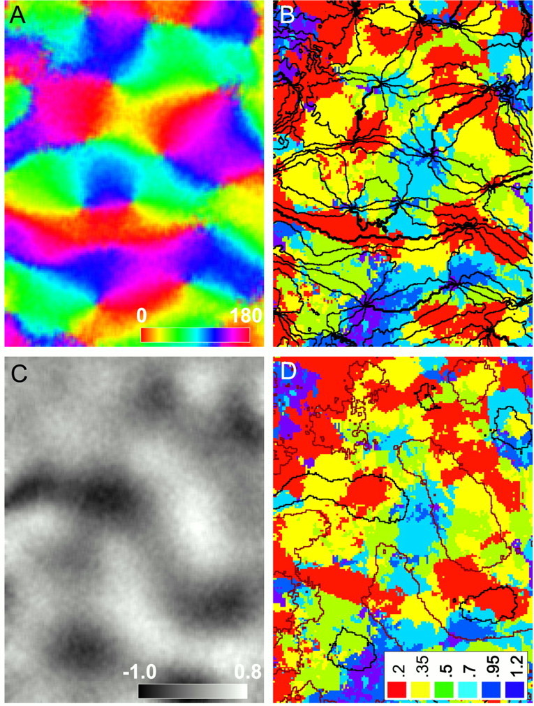
Comparison of orientation and ocular dominance maps with the spatial frequency map. A, Orientation preference is represented by color in this smoothed angle map. Thecolor bar represents orientation preference in degrees. The length of the color bar corresponds to 1 mm. This orientation map was constructed using square wave gratings of fundamental SF 0.2 c/°. B, SF map with iso-orientation contour lines overlaid. Points at which iso-orientation contours converge are the orientation pinwheel centers. Note that the color under most pinwheel centers is red orpurple, indicating an association between pinwheel centers and regions of low (red) and high (purple) SF preference. C, In this ocular dominance ratio map, dark areas are dominated by the ipsilateral eye, and light areas are dominated by the contralateral eye. Thegrayscale bar shows the deviation of pixel intensities ( ×10⁴) from 1.0, the value corresponding to equal activation by the two eyes. D, SF map with ocular dominance contours overlaid. No clear association was observed between the SF and ocular dominance maps. Thelegend shows the SF preference color code for the SF map shown in B and D.

A correlation between the positions of ocular dominance column peaks and orientation pinwheel centers has been observed in cat V1 (Crair et al., 1997a; Hubener et al., 1997). Based on this correlation and a previous finding that low SF domains tend to lie in the center of ocular dominance columns (Hubener et al., 1997), we expected that the peaks of ocular dominance columns would be differentially distributed across SF domains, perhaps in a similar manner to pinwheel centers. Visual inspection of the example maps in Figure 6, C andD, however, shows little correlation between ocular dominance columns and specific SF domains. To verify this quantitatively, we measured the density of ocular dominance peaks that lay within regions of cortex that preferred each SF. Although the density of ocular dominance column peaks was larger in low (2.6 peaks/mm²) SF domains than in either intermediate (1.8 peaks/mm²) or high (1.5 peaks/mm²) SF domains, this distribution was not statistically different from random [χ²(2) = 2.80; p = 0.25; n = 64 peaks].

The dependence of spatial frequency preference on stimulus orientation

Our characterizations of SF preference presented thus far have relied on a definition of SF preference that does not assume that SF preference is constant across all stimulus orientations. Specifically, SF preference has been defined only at a single orientation, the preferred orientation of a pixel. Other studies of SF preference have averaged responses over all orientations (Tootell et al., 1981; Hubener et al., 1997; Shoham et al., 1997; Everson et al., 1998), implicitly assuming that SF preference is independent of stimulus orientation and therefore that the averaging preserves SF preference in the map. Preferred SF is, however, not independent of stimulus orientation for many single units (Webster and De Valois, 1985).

To test explicitly whether SF preference measured optically is independent of stimulus orientation, we constructed SF tuning curves at a variety of stimulus orientations. Figure7A–C compares responses to different SFs for stimuli at the preferred orientation of each pixel with responses to stimuli at orientations that differ from the preferred by 22 or 45°. Each panel shows responses compiled from all of the pixels in the map of the case illustrated in Figure 2 that prefer a low SF (A), an intermediate SF (B), or a high SF (C) at their optimal orientation. In every case, the strongest response by far occurs at the preferred orientation (curves marked0), and it is clear that the tuning curve for SF is much broader at off-peak orientations. C shows that the peak response shifts to progressively lower SFs as the stimulus orientation changes from the optimal. D plots the change in the preferred SF as a function of stimulus orientation for all of the pixels in the map. For the regions of cortex that preferred high SFs, the curves fall off sharply as orientation changes in either direction, indicating preference for lower SFs at nonoptimal orientations. This behavior is predicted by linear models of simple cell receptive fields (Webster and De Valois, 1985). Only the lowest two SFs (≤0.35 c/°) do not fall off as orientation changes. Overall, the assumption that SF tuning is independent of stimulus orientation is wrong; there are systematic shifts in SF preference at off-peak orientations.

The independence of orientation preference from stimulus spatial frequency

Consistent with single-unit studies (Webster and De Valois, 1985), orientation preference has been assumed to be independent of stimulus SF in almost all optical measurements of orientation maps. To investigate the dependence of orientation preference on the SF of a stimulus, we constructed an angle map for each of six stimulus spatial frequencies (Fig. 8). Inspection of the six angle maps in Figure 8 shows that orientation preference changes little with stimulus spatial frequency. To quantitatively assess the difference between angle maps produced by stimulation at different spatial frequencies, we calculated for each pixel in the map the SD of orientation preference over the six SFs. In the angle map in Figure 8,bottom row, the average orientation preference of a pixel is represented by its color and its SD in orientation by its brightness (the darker the pixel, the larger the SD). Nearly all of the pixels in the map are bright, suggesting that orientation preference is primarily independent of stimulus SF. The distribution of these SDs is plotted in the histogram in Figure 8 and shows that ∼80% of the pixels in the map have an SD less than the sampling interval of 22.5°. Although the analysis presented in the previous section shows that SF preference is dependent on stimulus orientation, this demonstration shows that the converse is not true; orientation preference is independent of stimulus SF.

Fig. 8.

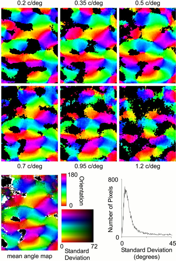
The effect of stimulus spatial frequency on orientation preference. The six angle maps in the top two rows were constructed using sinusoidal gratings with the SF shown with each map. Black areas in these maps had a peak activity below the 2ς threshold (as in Fig. 4). The average orientation preference and the SD in orientation preference for these maps is shown in the mean angle map panel. In this map, orientation preference is denoted by pixel hue, and SD is denoted by pixel brightness (the darker the pixel, the larger the SD). Pixels on the map that are black had no responses above threshold in any of the six maps and therefore have no mean orientation preference; pixels that are whitehave only one angle map contributing to the mean and therefore have no SD. The distribution of SDs is shown in the histogram.

Computation of spatial frequency maps using other algorithms

The choice of analysis procedure affects the appearance of SF maps. The two previous groups that reported on SF tuning using optical imaging (Hubener et al., 1997; Shoham et al., 1997; Everson et al., 1998) used analysis procedures that tacitly assumed that averaging responses to stimulation at all orientations would not affect the determination of SF preference at each point in cortex. In contrast, we analyzed the SF tuning only at the preferred orientation of the cortical cells underlying each pixel, a procedure identical to that used in characterizing SF preference electrophysiologically. The analysis below shows that the differences between our SF maps and those of the other groups result, in part, from the algorithms used to compute SF maps. When we analyze our responses with their algorithms, we can reproduce their findings.

Figure 9, A and B, compares an SF map constructed using the procedure described for Figure5E (selecting the preferred orientation and estimating an SF preference based on the SF tuning curve; Fig. 9A) to an SF map constructed by first averaging responses over all orientations and then estimating an SF preference based on the resulting SF tuning curve (Fig. 9B). Unlike the pattern of SF domains in Figure9A, SF domains in Figure 9B are arranged in SF pinwheels, similar to those described by Everson et al. (1998). Because these pinwheels are not present in Figure 9A, we conclude that they are produced by averaging over all orientations, because that is the difference between the computations in Figure 9, Aand B. The SF map of Everson et al. (1998) therefore does not represent only SF preference; rather, it is a map that combines SF preference with the dependence of SF preference on stimulus orientation.

Fig. 9.

Comparison with previous analyses of optical SF responses. A, An interpolated SF map constructed using the techniques described in Materials and Methods. B, An interpolated SF map constructed by first averaging over all orientations and then interpolating between SFs to get the preferred SF. SF pinwheels similar to those found by Everson et al. (1998) can be seen in this map. C, An SF response map constructed by selecting the preferred SF at the preferred orientation. Pixellightness is proportional to response strength. This map uses blank-screen normalization with no averaging over orientation.D, An SF response map constructed by normalizing single-condition images to a cocktail blank, averaging the response of a pixel over all orientations and then selecting the SF that most strongly activated the pixel [similar to the protocols of Hubener et al. (1997) and Shoham et al. (1997)]. Pixel lightnessis proportional to response strength. There are fewer bright pixels at intermediate SFs than there are in the map of C.E, Response amplitude as a function of preferred SF for the map shown in C. The red linewith open circles shows the distribution of average response amplitudes as a function of spatial frequency. Note that responses are greatest for intermediate SFs. The blue line with filled symbols is calculated from a subset of the data containing all but the highest two SFs (1.2 and 1.84 c/°). Note that response intensities for the truncated and complete data set are nearly identical. F, Response amplitude as a function of preferred SF for the map shown in D. The dashed red line with open triangles shows the distribution of average response amplitudes as a function of spatial frequency. Response amplitudes are weakest for intermediate SFs, unlike the profile inE. The depth of the trough shown in the profile depends on the noise threshold used to generate the SF map; maps generated using a lower threshold, and therefore excluding fewer points from analysis, would have a response profile with a shallower trough. Thedashed blue line is calculated from a subset of the data containing all but the highest two SFs (1.2 and 1.84 c/°; using the same threshold level) and shows a peak at 0.8 c/°. This profile is completely different from the one shown in red, calculated from the entire data set. Cocktail-blank normalization therefore makes the response profile dependent on the particular stimulus set used for analysis.

The SF maps produced by Shoham et al. (1997) and Hubener et al. (1997)can also be reproduced by duplicating their analytical procedures. In addition to averaging over all stimulus orientations, these groups used a normalizing procedure known as cocktail-blank normalization. With cocktail-blank normalization, images of responses to individual stimuli are divided by the mean image of all responses in the particular stimulus set. Figure 9C shows an SF response map similar to that shown in Figure 3. Figure 9D shows the same data analyzed with the procedures of Shoham et al. (1997) and Hubener et al. (1997). Compared with the map in Figure 9C, the SF map in Figure 9D has fewer areas that prefer intermediate SFs.

Cocktail-blank normalization has two effects on the SF maps. First, it preferentially reduces responses to intermediate SFs. As an example of this problem, consider the effect of cocktail-blank normalization on the responses of three pixels (their responses to stimuli of low, intermediate, or high SF are given in parenthesis): one that prefers a low SF (response of 1, 0.5, and 0), one that prefers an intermediate SF (response of 0.5, 1, and 0.5), and one that prefers a high SF (response of 0, 0.5, and 1). Normalizing the peak response of each pixel by its average response reduces the peak response for the pixel that prefers an intermediate SF (peak response intensities after normalization of 2, 1.5, and 2 for the pixel that prefers a low, intermediate, and high SF, respectively).

This first effect, the reduction in response to intermediate SFs, can be seen for the data shown in Figure 9D (compare withC, which has no cocktail-blank normalization or averaging over orientations). The open symbols in Figure 9Eshow the mean response intensities in domains that prefer different SFs for the map in 9C. The strongest responses occur at intermediate SFs. The open symbols in Figure 9Fshow the same plot for the map in Figure 9D. It is clear that the strongest response occur at the extremes of the SF range in this plot. Thus, the combined effect of averaging over all orientations and cocktail-blank normalization is to reduce the apparent response strength of the pixels that prefer intermediate SFs.

The second effect of cocktail-blank normalization is that apparent response intensities are dependent on the specific set of stimuli used. Because the cocktail blank (which is the mean image to which all images are normalized) is composed of the responses to a specific set of stimuli, changing the stimulus set changes the apparent responses. To demonstrate this dependence, we recalculated the mean response strengths for the data presented in Figure 9, C andD, using the range of SFs studied by Shoham et al. (1997), i.e., a subset of our stimuli that did not include the two highest SFs of 1.2 and 1.84 c/°. Using our blank-normalization procedure, the response profile calculated for the truncated data set changed little from the responses calculated from the entire data set (Fig.9E, compare blue line, red line). In contrast, using cocktail-blank normalization, the response profile was completely different for the truncated data set compared with the entire data set (Fig. 9F, compare blue line,red line). Indeed, the truncated data set normalized by the cocktail blank produces a profile almost exactly matching that described by Shoham et al. (1997); only pixels that prefer very low or high SFs appear strongly active. Thus, analyzing different portions of the data set gives very different maps and conclusions if one averages over orientations and uses cocktail-blank normalization. In contrast, our assessment of SF responses at the optimal orientation and with true blank-screen normalization produces a unique map and response profile that does not depend on the particular stimulus set used.

DISCUSSION

Four rules characterize the organization of SF preference in V1. First, cells with SF preferences between 0.2 and 1.8 c/° are clustered into domains with other cells of similar SF preference. Cells in these domains respond well only to spatial frequencies within one to two octaves of the preferred SF. Second, these SF domains are organized into a map that is locally continuous across V1, although the spatial gradient of SF preference is not constant, and there are often clear fractures in the SF map before the entire range of SF preference is represented. Third, although SF domains are irregularly spaced, the distance between domains of very different SF preference conforms to the hypercolumn description of cortical organization. Finally, cortical domains containing cells that prefer the extremes of the SF continuum, either very low or very high spatial frequencies, tend to colocalize with the pinwheel center singularities in the cortical map of orientation preference.

Several observations confirm that the optically derived maps accurately represent the SF preference of neurons in V1. First, the same optical data that we analyzed for SF also produced maps of orientation preference that were consistent with the known cortical organization. Second, the observed SF maps were consistent with the gross layout and distribution of SF preference in visual cortex as demonstrated by previous electrophysiological and optical imaging experiments (Movshon et al., 1978b; Bonhoeffer et al., 1995). Finally, our optical maps of SF preference were closely correlated with findings from targeted microelectrode penetrations measuring SF preference in neurons of the supragranular layers of V1 (Fig. 3).

Comparison with previous imaging studies of spatial frequency maps in V1

The maps of SF preference described here differ from the results of previous imaging studies. In one such study, Everson et al. (1998)concluded that the SF map in V1 contains pinwheel centers around which all SF preferences are represented. Although we have found places in SF maps at which several SF domains meet, these are generally not pinwheel centers, because only a few SFs are represented around the junction point. Instead, we have found that the extremes of the SF map (high and low SFs) rarely meet and are usually separated by domains of intermediate SF preference. Indeed, we have found that the apparent pinwheel organization observed by Everson et al. (1998) can be produced by averaging SF responses over all stimulus orientations (Fig.9B). These maps thus combine a representation of preferred SF with significant effects of orientation tuning, SF tuning, and the complex relationship between these features.

Shoham et al. (1997) noted “rather than observing a map of continuously changing spatial frequency preference across the cortical surface … found only two distinct sets of domains, one preferring low spatial frequency … and the other high spatial frequency.” Our description of cortical SF preference differs from that of Shoham et al. (1997) and Hubener et al. (1997) by the inclusion of domains with distinct preferences for intermediate SFs. Indeed, some of the strongest responses we have measured come from these intermediate SF domains. Two lines of evidence support the existence of cortical regions selective for any of a wide range of SFs. First, recordings from microelectrode penetrations targeted to SF domains were consistent with the SF preference measured from the optical map. Because we found a broad range of SF preferences with both electrophysiological and optical techniques, it is unlikely that the observed intermediate SF domains (between 0.3 and 0.8 c/°) are artifacts of intrinsic signal imaging. Second, the SF tuning curves measured in intermediate SF domains cannot be reproduced by a linear summation of the tuning curves from the high and low SF domains (Fig. 4). This rules out the possibility that intermediate SF domains are produced simply by the overlap of neighboring high and low SF domains and suggests that the intermediate SF domains exist independently of neighboring domains.

Several differences in experimental protocols and in analytic procedures may account for the differences between the SF maps described here and those of Shoham et al. (1997) and Hubener et al. (1997). First, we used a larger range of spatial frequencies than did Shoham et al. or Hubener et al. Responses to the extremes of the SF range revealed domains preferring SFs higher than those tested by Shoham et al. or Hubener et al. Second, the conclusions of Hubener et al. were based on ratio maps in which only two different spatial frequencies were used, one “low” and the other “high.” Third, like Everson et al. (1998), Shoham et al. and Hubener et al. considered responses to different SFs after averaging these responses over all the orientations.

The final procedural difference is in the type of image normalization used in constructing maps of SF preference. Both Shoham et al. and Hubener et al. used cocktail-blank normalization, whereas we used blank stimulus normalization. Cocktail-blank normalization can accentuate differences in responses to certain stimuli, but it can also obscure genuine responses (compare the conclusions of Crair et al., 1997b with those of Kim and Bonhoeffer, 1994). Cocktail-blank normalization specifically reduces the response intensity of intermediate SFs, and the degree of this reduction depends on the exact set of stimuli used in mapping spatial frequency. If few stimuli with closely spaced SFs are used to map SF preference, only the extremes of the SF range will produce strong responses (Fig. 9F, blue line). If several stimuli spread out over a large range of SF are used, there is still a reduction in response to intermediate SFs, but the reduction is less pronounced (Fig. 9F, red line). Cocktail-blank-normalized SF maps therefore fail to describe the underlying structure of SF preference because they necessarily have a reduced representation of intermediate SFs and because they have a structure dictated by the specific stimuli used for analysis instead of by the SF preferences of the cells in the cortex.

Despite disagreement between our results and those of Shoham et al. (1997) and Hubener et al. (1997) over the extent of high and low SF domains, these domains defined with optimally oriented stimuli and blank-screen normalization usually fall within the high and low SF domains produced by averaging over orientations and normalizing by the cocktail blank. Because there is little disagreement over the gross positions of these domains, our results provide no reason to doubt the general relationship between cytochrome oxidase blobs and low SF domains proposed by Shoham et al. (1997). Moreover, we have come to a similar conclusion as Hubener et al. (1997) that there is an association between pinwheel centers and domains of high and low SF preference. We have also found a trend, not statistically significant in our maps, for an association between peaks of ocular dominance and low SF domains, as proposed by Hubener et al. (1997).

Implications for development of receptive fields and cortical maps

Geniculocortical X and Y cells have different SF tuning characteristics. The response of the Y cell to visual stimuli has a low SF cutoff (corner frequency of first harmonic response of 0.4 c/°) (Derrington and Fuchs, 1979), whereas the X cell has a higher low-pass cutoff (corner frequency of 1 c/°) (Derrington and Fuchs, 1979). This difference in SF filtering properties was proposed to underlie a role for X and Y type thalamocortical projections in determining the structure of the cortical SF map. SF maps that appeared to show only high and low SF domains (Shoham et al., 1997) seemed consistent with a tangential partition of the cortex into domains receiving input from X or Y cells, despite anatomical evidence of a sublaminar rather than tangential segregation of X and Y input (for review, see Sherman, 1985). Our finding that the full range of SF preferences is mapped continuously across V1 makes it unlikely that a bimodal segregation of X and Y inputs accounts for the pattern of the cortical SF map.

What might be the value of the relationship between low and high SF domains and orientation pinwheels found in the present study and byHubener et al. (1997)? The colocalization of pinwheel centers and the extrema of the SF map may have functional relevance. Only a small area of cortex is devoted to the extrema of SF. Centering these extrema of the SF map on the pinwheels ensures that all orientations are represented at those rarer spatial frequencies. Consider the alternative: if these extremes of SF were represented away from the pinwheels, then they might well fall within a single orientation domain, causing those spatial frequencies to fail to be represented for other stimulus orientations in a portion of the visual field. The actual arrangement has the additional benefit that, because the mapping of SF is mostly continuous, the less extreme SFs tend to be arrayed around the pinwheels, thereby covering the full range of orientations. The relationship between the orientation and SF maps may, therefore, ensure that all orientations are represented at all spatial frequencies.

If the relationship between the orientation and SF maps is consistent across species, it may provide an important constraint to models of V1 development. Predicting the shape of the orientation map alone is not sufficient to validate the assumptions of a model; nearly any mixture of spatially periodic orientation domains will produce a pinwheel-like structure (Rojer and Schwartz, 1990) (for discussion, see Miller, 1994). Models that reproduce the combined pattern of SF and orientation maps are more likely to provide biologically relevant insights into map development and function.

Comparison with microelectrode and behavioral studies of spatial frequency in V1

The range of SF preferences found in optical maps is consistent with the findings of many electrophysiological and behavioral studies on SF preference in the cat. There is a wide range of preferred SFs among neurons in V1 (Movshon et al., 1978b; Tolhurst and Thompson, 1981; Robson et al., 1988), and cortical neurons with similar SF preference are clustered (Tolhurst and Thompson, 1982; De Angelis et al., 1999). Together, these findings would predict the type of SF domains observed in Figures 2, 3, and 5. It is interesting to note, however, that the highest SF preference observed in these imaging experiments (∼1.8 c/°) is significantly lower than the highest SF responses observed with single-unit recording (∼3 c/°) (Movshon et al., 1978b). This discrepancy is likely attributable to the fact that the activity measured at each pixel is an average of activity from many neurons. Because the fraction of neurons with the highest SF preference is small (Movshon et al., 1978b) and these neurons are likely buried at the center of high SF domains, it is unlikely that their activity would be resolved using intrinsic signal imaging.

Implications for cortical processing in V1

The clustering of cells with similar SF preferences in a continuous map in V1 is consistent with features of SF adaptation observed in human psychophysical studies (for review, see Shapley and Lennie, 1985; De Valois and De Valois, 1988) in which SF channels observed psychophysically might correspond to clusters of cells in V1 with similar SF preference. Adapting a viewer to a single SF degrades contrast sensitivity for a range of SFs centered on the adapting SF (Blakemore and Campbell, 1969). Because nearby cells in V1 have similar SF preferences, local interactions are primarily limited to similar SFs. Increased local inhibition would, therefore, affect only a limited range of SFs. If a common network of local corticocortical connections underlies this and other types of adaptation (adaptation to orientation or position for example), then the characteristic bandwidth of these adaptation effects (in SF space, orientation space, or retinotopic space) should be a single function of cortical distance.

REFERENCES

- 1.Anderson PA, Olavarria J, Van Sluyters RC. The overall pattern of ocular dominance bands in cat visual cortex. J Neurosci. 1988;8:2183–2200. doi: 10.1523/JNEUROSCI.08-06-02183.1988. [DOI] [PMC free article] [PubMed] [Google Scholar]
- 2.Blakemore C, Campbell FW. On the existence of neurones in the human visual system selectively sensitive to the orientation and size of retinal images. J Physiol (Lond) 1969;203:237–260. doi: 10.1113/jphysiol.1969.sp008862. [DOI] [PMC free article] [PubMed] [Google Scholar]
- 3.Bonhoeffer T, Grinvald A. Iso-orientation domains in cat visual cortex are arranged in pinwheel-like patterns. Nature. 1991;353:429–431. doi: 10.1038/353429a0. [DOI] [PubMed] [Google Scholar]
- 4.Bonhoeffer T, Grinvald A. Optical imaging based on intrinsic signals. In: Toga AW, Mazziotta JC, editors. Brain mapping: the methods. Academic; New York: 1996. pp. 55–97. [Google Scholar]
- 5.Bonhoeffer T, Kim D-S, Malonek D, Shoham D, Grinvald A. Optical imaging of the layout of functional domains in area 17 and across the area 17/18 border in cat visual cortex. Eur J Neurosci. 1995;7:1973–1988. doi: 10.1111/j.1460-9568.1995.tb00720.x. [DOI] [PubMed] [Google Scholar]
- 6.Crair MC, Ruthazer ES, Gillespie DC, Stryker MP. Ocular dominance peaks at pinwheel center singularities of the orientation map in cat visual cortex. J Neurophysiol. 1997a;77:3381–3385. doi: 10.1152/jn.1997.77.6.3381. [DOI] [PubMed] [Google Scholar]
- 7.Crair MC, Ruthazer ES, Gillespie DC, Stryker MP. Relationship between the ocular dominance and orientation maps in visual cortex of monocularly deprived cats. Neuron. 1997b;19:307–318. doi: 10.1016/s0896-6273(00)80941-1. [DOI] [PubMed] [Google Scholar]
- 8.De Angelis GC, Ghose GM, Ohzawa I, Freeman RD. Functional micro-organization of primary visual cortex: receptive field analysis of nearby neurons. J Neurosci. 1999;19:4046–4064. doi: 10.1523/JNEUROSCI.19-10-04046.1999. [DOI] [PMC free article] [PubMed] [Google Scholar]
- 9.De Valois R, De Valois K. Spatial vision. Oxford UP; New York: 1988. [Google Scholar]
- 10.Derrington AM, Fuchs AF. Spatial and temporal properties of X and Y cells in the cat lateral geniculate nucleus. J Physiol (Lond) 1979;293:347–364. doi: 10.1113/jphysiol.1979.sp012893. [DOI] [PMC free article] [PubMed] [Google Scholar]
- 11.Derrington AM, Fuchs AF. The development of spatial-frequency selectivity in kitten striate cortex. J Physiol (Lond) 1981;316:1–10. doi: 10.1113/jphysiol.1981.sp013767. [DOI] [PMC free article] [PubMed] [Google Scholar]
- 12.Everson RM, Prashanth AK, Gabbay M, Knight BW, Sirovich L, Kaplan E. Representation of spatial frequency and orientation in the visual cortex. Proc Natl Acad Sci USA. 1998;95:8334–8338. doi: 10.1073/pnas.95.14.8334. [DOI] [PMC free article] [PubMed] [Google Scholar]
- 13.Graham H, Nachmias J. Detection of grating pattern containing two spatial frequencies: a comparison of single channel and multichannel models. Vision Res. 1971;11:251–259. doi: 10.1016/0042-6989(71)90189-1. [DOI] [PubMed] [Google Scholar]
- 14.Hubel DH, Wiesel TN. Receptive fields, binocular interaction, and functional architecture in the cat's visual cortex. J Physiol (Lond) 1962;160:106–154. doi: 10.1113/jphysiol.1962.sp006837. [DOI] [PMC free article] [PubMed] [Google Scholar]
- 15.Hubel DH, Wiesel TN. Uniformity of monkey striate cortex: a parallel relationship between field size, scatter, and magnification factor. J Comp Neurol. 1974;158:295–306. doi: 10.1002/cne.901580305. [DOI] [PubMed] [Google Scholar]
- 16.Hubener M, Shoham D, Grinvald A, Bonhoeffer T. Spatial relationships among three columnar systems. J Neurosci. 1997;1997:9270–9284. doi: 10.1523/JNEUROSCI.17-23-09270.1997. [DOI] [PMC free article] [PubMed] [Google Scholar]
- 17.Issa NP, Trachtenberg JT, Chapman B, Zahs KR, Stryker MP. The critical period for ocular dominance plasticity in the ferret's visual cortex. J Neurosci. 1999;19:6965–6978. doi: 10.1523/JNEUROSCI.19-16-06965.1999. [DOI] [PMC free article] [PubMed] [Google Scholar]
- 18. Kim DS, Bonhoeffer T. Reverse occlusion leads to a precise restoration of orientation preference maps in visual cortex. Nature 370 1994. 370 372[Erratum (1994) 372:196]. [DOI] [PubMed] [Google Scholar]
- 19.Kulikowski JJ, Bishop PO. Linear analysis of the responses of simple cells in the cat visual cortex. Exp Brain Res. 1981;44:386–400. doi: 10.1007/BF00238831. [DOI] [PubMed] [Google Scholar]
- 20.LeVay S, Nelson SB. Columnar organization of the visual cortex. In: Leventhal AG, editor. The neural basis of visual function. CRC; Boston: 1991. pp. 266–315. [Google Scholar]
- 21.LeVay S, Stryker MP, Shatz CJ. Ocular dominance columns and their development in layer IV of the cat's visual cortex: a quantitative study. J Comp Neurol. 1978;179:223–244. doi: 10.1002/cne.901790113. [DOI] [PubMed] [Google Scholar]
- 22.Maffei L, Fiorentini A. Spatial frequency rows in the striate visual cortex. Vision Res. 1977;17:257–264. doi: 10.1016/0042-6989(77)90089-x. [DOI] [PubMed] [Google Scholar]
- 23.Miller K. A model for the development of simple cell receptive fields and the ordered arrangement of orientation columns through activity-dependent competition between ON- and OFF-center inputs. J Neurosci. 1994;14:409–441. doi: 10.1523/JNEUROSCI.14-01-00409.1994. [DOI] [PMC free article] [PubMed] [Google Scholar]
- 24.Movshon JA, Thompson ID, Tolhusrt DJ. Spatial summation in the receptive fields of simple cells in the cat's striate cortex. J Physiol (Lond) 1978a;283:53–77. doi: 10.1113/jphysiol.1978.sp012488. [DOI] [PMC free article] [PubMed] [Google Scholar]
- 25.Movshon JA, Thompson ID, Tolhusrt DJ. Spatial and temporal contrast sensitivity of neurones in areas 17 and 18 of the cat's visual cortex. J Physiol (Lond) 1978b;283:101–130. doi: 10.1113/jphysiol.1978.sp012490. [DOI] [PMC free article] [PubMed] [Google Scholar]
- 26.Obermayer K, Blasdel GG. Geometry of orientation and ocular dominance columns in monkey striate cortex. J Neurosci. 1993;13:4114–4129. doi: 10.1523/JNEUROSCI.13-10-04114.1993. [DOI] [PMC free article] [PubMed] [Google Scholar]
- 27.Robson JG, Tolhurst DJ, Freeman RD, Ohzawa I. Simple cells in the visual cortex of the cat can be narrowly tuned for spatial frequency. Vis Neurosci. 1988;1:415–419. doi: 10.1017/s095252380000417x. [DOI] [PubMed] [Google Scholar]
- 28.Rojer AS, Schwartz EL. Cat and monkey cortical columnar patterns modeled by bandpass-filtered 2D white noise. Biol Cybern. 1990;62:381–391. doi: 10.1007/BF00197644. [DOI] [PubMed] [Google Scholar]
- 29.Sachs MB, Nachmias J, Robson JG. Spatial frequency channels in human vision. J Opt Soc Am. 1971;61:1176–1186. doi: 10.1364/josa.61.001176. [DOI] [PubMed] [Google Scholar]
- 30.Shapley R, Lennie P. Spatial frequency analysis in the visual system. Annu Rev Neurosci. 1985;8:547–583. doi: 10.1146/annurev.ne.08.030185.002555. [DOI] [PubMed] [Google Scholar]
- 31.Sherman SM. Functional organization of the W-, X-, and Y-cell pathways in the cat: a review and hypothesis. In: Sprague JM, Epstein AN, editors. Progress in psychobiology and physiological psychology, Vol 11. Academic; NewYork: 1985. pp. 233–314. [Google Scholar]
- 32.Shoham D, Hubener M, Schulze S, Grinvald A, Bonhoeffer T. Spatio-temporal frequency domains and their relation to cytochrome oxidase staining in cat visual cortex. Nature. 1997;385:529–533. doi: 10.1038/385529a0. [DOI] [PubMed] [Google Scholar]
- 33.Silverman MS. PhD thesis. University of California, San Francisco, CA; 1984. Deoxyglucose and electrophysiological evidence for spatial frequency columns in cat striate cortex. [Google Scholar]
- 34.Stone J, Dreher B, Leventhal A. Hierarchical and parallel mechanisms in the organization of the visual cortex. Brain Res Rev. 1979;1:345–394. doi: 10.1016/0165-0173(79)90010-9. [DOI] [PubMed] [Google Scholar]
- 35.Tang Y, Norcia AM. Improved processing of the steady-state evoked potential. Electroencephalogr Clin Neurophysiol. 1993;88:323–334. doi: 10.1016/0168-5597(93)90056-u. [DOI] [PubMed] [Google Scholar]
- 36.Thompson ID, Kossut M, Blakemore C. Development of orientation columns in cat striate cortex revealed by 2-deoxyglucose autoradiography. Nature. 1983;301:712–715. doi: 10.1038/301712a0. [DOI] [PubMed] [Google Scholar]
- 37.Tolhurst DJ, Thompson ID. On the variety of spatial frequency selectivities shown by neurons in area 17 of the cat. Proc R Soc Lond B Biol Sci. 1981;213:183–199. doi: 10.1098/rspb.1981.0061. [DOI] [PubMed] [Google Scholar]
- 38.Tolhurst DJ, Thompson ID. Organization of neurones preferring similar spatial frequencies in cat striate cortex. Exp Brain Res. 1982;48:217–227. doi: 10.1007/BF00237217. [DOI] [PubMed] [Google Scholar]
- 39.Tootell RB, Silverman MS, De Valois RL. Spatial frequency columns in primary visual cortex. Science. 1981;214:813–815. doi: 10.1126/science.7292014. [DOI] [PubMed] [Google Scholar]
- 40.Trepel C, Issa NP, Stryker MP. Spatial frequency maps in cat primary visual cortex. Soc Neurosci Abstr. 1999;572:10. doi: 10.1523/JNEUROSCI.20-22-08504.2000. [DOI] [PMC free article] [PubMed] [Google Scholar]
- 41.Watson AB. Summation of grating patches indicates many types of detectors at one retinal location. Vision Res. 1982;22:17–25. doi: 10.1016/0042-6989(82)90162-6. [DOI] [PubMed] [Google Scholar]
- 42.Watson AB, Robson JG. Discrimination at threshold: labelled detectors in human vision. Vision Res. 1981;21:1115–1122. doi: 10.1016/0042-6989(81)90014-6. [DOI] [PubMed] [Google Scholar]
- 43.Webster MA, De Valois RL. Relationship between spatial-frequency and orientation tuning of striate-cortex cells. J Opt Soc Am A. 1985;2:1124–1132. doi: 10.1364/josaa.2.001124. [DOI] [PubMed] [Google Scholar]