Compliance, actuation, and work characteristics of the goat foreleg and hindleg during level, uphill, and downhill running

Abstract

We model the action of muscle-tendon system(s) about a given joint as a serial actuator and spring. By this technique, the experimental joint moment is imposed while the combined angular deflection of the actuator and spring are constrained to match the experimental joint angle throughout the stance duration. The same technique is applied to the radial leg (i.e., shoulder/hip-to-foot). The spring constant that minimizes total actuator work is considered optimal, and this minimum work is expressed as a fraction of total joint/radial leg work, yielding an actuation ratio (AR; 1 = pure actuation and 0 = pure compliance). To address work modulation, we determined the specific net work (SNW), the absolute value of net divided by total work. This ratio is unity when only positive or negative work is done and zero when equal energy is absorbed and returned. Our proximodistal predictions of joint function are supported during level and 15° grade running. The greatest AR and SNW are found in the proximal leg joints (elbow and knee). The ankle joint is the principal spring of the hindleg and shows no significant change in SNW with grade, reflecting the true compliance of the common calcaneal tendon. The principal foreleg spring is the metacarpophalangeal joint. The observed pattern of proximal actuation and distal compliance, as well as the substantial SNW at proximal joints, minimal SNW at intermediate joints, and variable energy absorption at distal joints, may emerge as general principles in quadruped limb mechanics and help to inform the leg designs of highly capable running robots.

During level running, the legs of animals shorten as they are loaded, then rebound as they are unloaded. This inverse relationship between leg length and leg force suggests a simple springlike leg function, but such conservative mechanics cannot sustain locomotion on a grade. Uphill and downhill running require net propulsive and braking forces, respectively, to resist the component of gravity parallel to the slope. Consequently, net work against gravity may be required of the joints that flex and extend to shorten and lengthen the leg. This report investigates spring characteristics, as well as patterns of actuation and work, of the joints and legs during level, uphill, and downhill running. On the basis of the anatomic distribution of long tendons (distal) vs. large muscles with short tendons and longer fibers (proximal), a central hypothesis of this study predicts greater compliance in distal joints and greater actuation in proximal joints.

Spring characteristics of the knee, ankle, and leg have been examined in humans using a number of different experimental and analytical approaches. Ankle spring constants were first determined for running and sprinting by Stefanyshyn and Nigg (40), revealing increased stiffness of the ankle during sprinting compared with running. Arampatzis and coworkers (2) determined joint and leg spring constants over a range of running speeds and concluded that knee and leg spring constants tend to increase with speed, while the ankle spring constant is unchanged. These results suggest that leg stiffness tends to be actively modulated by the knee during running, whereas increased ankle stiffness may be a unique feature of sprinting vs. running. In agreement with Arampatzis et al. (2) and in contrast to Stefanyshyn and Nigg (40), humans were found to have consistent ankle spring constants but increasing knee spring constants over a range of sprinting speeds (70–100% of maximum) (24). These authors suggest that ankle spring constant is dominated by the intrinsic compliance of the triceps surae muscle-tendon complex. Gunther and Blickhan (19) found a greater linearity in the ankle than in the knee spring during running, further supporting the idea of a simpler springlike function of the more distal ankle and a greater scope for mechanical modulation in the more proximal knee. Leg spring constants have also been found to change to accommodate substrates of variable stiffness, but the contributions of individual joints to this modulation are not fully understood (12, 13).

As shown by Arampatzis et al. (2), leg spring constants determined by direct measurement of leg deflection and leg force differ from spring constants determined by the spring-mass model of McMahon and Cheng (30), which depends on leg excursion angle to estimate leg deflection. Although it has been shown to underestimate leg spring constant in running humans (2), the spring-mass model has proven useful in characterizing running mechanics of two-, four-, six-, and eight-legged runners (4) and even provided an empirical power function for leg spring constant across an enormous size range of quadrupeds (11). In addition, the spring-mass model inspired the first fast running machines, built by Raibert (37) and coworkers, and continues to influence new generations of highly capable running robots.

Despite its great utility in comparing multilegged runners, the spring mass model requires a tenuous assumption when more than one limb is in contact with the ground: the choice of a single leg excursion angle to represent the combined action of multiple limbs. In an experimental running machine, this discrepancy was avoided by imposing foreleg-hindleg symmetry and controlling a quadruped according to the spring-mass mechanics of a virtual biped (37, 38). In living quadrupeds, however, forelimb-hindlimb function is asymmetrical (26, 27). Even though the center of mass (CoM) dynamics of trotting and pacing may resemble bipedal running, this is achieved by a fore- and hindlimb pair, rather than by a single contact limb. Furthermore, limb contacts are out of phase during faster running gaits, such as cantering and galloping (21), so no single limb adequately represents the spring-mass model.

Because of simultaneous contacts and asymmetry of individual limb function during quadrupedal running, we did not attempt to model the whole animal as a spring-mass system. Instead, we examined the mechanics of individual limbs during stance, focusing on specific joints and on the radial leg. In this report, “leg” or “radial leg” refers only to the portion of the limb between the shoulder or hip and the foot. Hence, the leg joints are those distal to the shoulder or hip, while the limb includes these proximal joints and the pectoral and pelvic girdles that bind them to the axial skeleton. It should be noted that “shoulder” refers to the scapulohumeral joint, rather than the scapula itself, which is typically visualized by x-ray imaging (14, 22). Unlike previous studies, which employed spring constant estimates from either peak joint moments and angular deflections or linear regression of joint moment on joint angle, we have incorporated a serial actuator-spring model to assess spring characteristics. To characterize level, uphill, and downhill running mechanics of goats, we report joint and radial leg spring constants along with three basic mechanical parameters: 1) actuation ratio (AR), the fraction of total joint (or radial leg) work done by the actuator in the serial actuator-spring model; 2) net work, the work contribution of a specific joint or radial leg; and 3) specific net work (SNW), the absolute value of net work as a fraction of total joint (or radial leg) work.

METHODS

Subjects and experimental procedures

Level, uphill, and downhill running steps were recorded from three adult female goats (Capra hircus, breed: African Pygmy) ranging in body mass from 21 to 26 kg. Level running was recorded on an indoor runway (10 m long) with a hard rubber surface, and slope running was recorded on an outdoor runway (8 m long) with a 15° grade and a packed soil surface. In both runways a pair of rectangular force platforms (0.6 × 0.4-m top dimensions) were embedded flush with the runway and oriented end to end with long axes parallel to the runway. Force platforms were covered with rubberized traction tape (3M Safety-Walk Medium Duty Resilient Tread 7741). Minimal training was required, as audible cues were sufficient to prompt the goats to run the length of the runway at various trotting and galloping speeds. The goats were given at least 2 min of rest at the opposite end of the runway before they were prompted to run back. All procedures for goat handling were approved by Harvard University’s Institutional Animal Care and Use Committee. Running footfalls were measured in both running directions from either left or right limbs. A total of 30 –50 trials was recorded from each subject, and subsequent analysis utilized all isolated footfalls from camera-facing fore- and hindlimbs. Footfalls that partially contacted either the surrounding runway or adjacent force platform were discarded.

A pair of Kistler type 9286AA force platforms mounted with thin epoxy foot moldings onto separate 3.2-cm-thick granite slabs was set into a trench in the indoor runway. A pair of AMTI BP400600HF force platforms bolted onto separate 2.5-cm-thick steel base plates was installed in the outdoor runway. These plates were set on a buried concrete slab with wooden side rails. A thin layer of sand prevented rocking, and recessed wooden rails prevented downslope slippage. Force data were sampled at 2,400 Hz for 5 s, using a manual pretrigger from the motion capture system. A BioWare type 2812A1-3 analog-to-digital (A/D) system (DAS1602/16 A/D board) operated using BioWare 3.0 software (Kistler Instruments) or two AMTI MSA-6 strain-gauge amplifiers with a National Instruments DAQCard 6036E and LabView 7.1 software were used to amplify, digitize, and save force platform data. During level and slope running experiments, a Qualisys three-dimensional (3-D) infrared system (3 ProReflex MCUs) and Qualisys Track Manager 1.6 software were used for motion capture. Retroreflective polystyrene hemispheres (covered with 3M 7610WS High Gain Sheeting) were used to mark the fore-and hindlimb joints, lateral hooves, iliac crests, and the dorsal spine midway between the limb girdles. The 3-D positions of these markers were recorded at 240 Hz.

Kinetic and kinematic parameters

The ground reaction force (GRF) normal to the platform surface (F_n) and the component of shear force in the direction of travel (F_s) were used in a planar kinetic analysis. (GRF directed toward the animal and forward in the direction of travel are considered positive.) Table 1 summarizes notation used in this report. Impulses (j_n and j_s) were determined by numerical integration of F_n and F_s over the contact time (t_c). The resultant angle (θ) of j_n and j_s, defined with respect to normal, is given by

Table 1.

Notation

Symbol	Unit of Measure	Definition
GRF	N	Ground reaction force
tc	s	Time of contact
Fn	N	Normal component of GRF
Fs	N	Shear component of GRF (direction of travel)
F̄	N	Mean resultant GRF magnitude
θ	deg (°)	Mean angle of resultant GRF with respect to normal
v̄	m/s	Mean forward (shear) velocity of the trunk
ϕj	rad	Joint angle
ωj	rad/s	Joint angular velocity
ωa	rad/s	Angular velocity of joint actuator
Mj	N 3 m	Joint moment
kj	N 3 m/deg	Joint spring constant
Lr	m	Radial leg length
Vr	m/s	Radial leg velocity
Va	m/s	Radial velocity of leg actuator
Fr	N	Radial leg force
kr	kN/m	Radial leg spring constant
W	J	Net work
|W|	J	Total work
AR		Actuation ratio
SNW		Specific net work

$$\theta ={tan}^{-1}(j_{\text{s}}/j_{\text{n}})$$ (1)

Hence, positive angles indicate propulsion and negative angles indicate braking. Mean magnitude of the resultant GRF was determined by

$$\overline{\mathbf{F}}=\sqrt{j_{\text{n}}^2+j_{\text{s}}^2}/t_{\text{c}}$$ (2)

As with GRF, kinematic analysis was restricted to the sagittal plane (defined by the normal axis and the shear axis in the direction of travel). Mean velocity in the direction of travel (v̄) was determined from the net trunk marker displacement during the contact time. Joint angle (ϕ_j) was determined from a joint marker and its adjacent markers that, together, define the two leg segments linked by the joint. Joint angular velocity (ω_j) was computed by differentiation of the joint angle with respect to time. By convention, flexing (i.e., closing) of a joint represents a decreasing joint angle. This directionality is illustrated in the individual joint models of Fig. 1. Note that joint rotation is the same in all three foreleg joints and in the distal hindleg joints, but knee rotation is opposite to these. Joint moments (M_j) were calculated as the determinant (i.e., cross product) of joint marker position (S_n, S_s) and GRF (F_n, F_s). Inertial and gravitational moments were neglected because of the extremely low mass and rotational inertia of the leg segments distal to elbow and knee and their minimal translational and rotational velocities during the stance phase (18, 32). The polarity of M_j was adjusted such that a moment tending to flex the joint is positive. This mirrors the joint angle convention; for example, flexing (negative angular deflection) under a positive moment represents negative joint work. Radial leg length (L_r) was determined as the distance from the proximal joint (shoulder or hip) to the hoof (Fig. 1). Leg radial velocity (V_r) was determined by differentiation with respect to time. Radial leg force (F_r) was determined by resolving F_n and F_s into the radial “axis” of the leg.

Fig. 1.

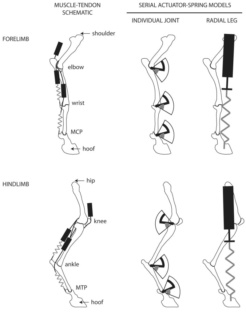
Simplified schematic representing the leg joints and muscle-tendon systems of the goat fore- and hind-limb. Black rectangles represent muscles, and gray lines represent long tendons that may act as springs. The serial actuator-spring model was applied to the individual joints (angular) and to the radial leg (i.e., a line from shoulder to foot or hip to foot). Black icons represent actuators, and gray icons represent springs. MCP and MTP refer to metacarpophalangeal joint and metatarso-phalangeal joint, respectively.

The serial actuator-spring model

We undertook a simple approach to characterizing the actuation and compliance of individual joints and the leg as whole. A Hookean spring in-series with an actuator represented the action of all of the muscle-tendon systems about a given joint or, in the case of the leg models, the combined action of multiple joints (Fig. 1). The phalanges with hoof were considered a single segment. Hence, four segments and three joints constituted the fore- and hindlimb joint models. The serial actuator-spring model for an individual joint is based on joint angular deflection and moment, while the serial actuator-spring model for the whole leg is based on radial deflection and radial force.

The serial actuator-spring model is described for the individual joint case in Fig. 2, using the ankle as an example. The experimentally measured M_j is imposed on the model throughout contact time. The spring deflects according to its spring constant k_j (or, in the radial leg model, k_r). The spring constants are determined iteratively, as described below. To maintain the experimentally measured, target angle θ_j (or, in the radial leg model, L_r), the actuator actively deflects to make up the difference between the modeled spring deflection and measured joint deflection. In the examples of Fig. 2, A–C, ankle moments and angles are shown during level, uphill, and downhill running trials from a single subject. Although optimal spring constants are consistent, there are clear mechanical differences across these locomotor conditions. Level running shows a roughly linear plot of M_j vs. ϕ_j, suggesting conservative, springlike mechanics. In contrast, uphill running shows greater angular extension under a greater flexing moment, with an M_j vs. ϕ_j plot showing substantial positive net work. During downhill running, the ankle flexes more than it extends and does negative net work. It is this diversity of mechanical behavior and potential underlying compliance that can be addressed with the serial actuator-spring model employed here.

Fig. 2.

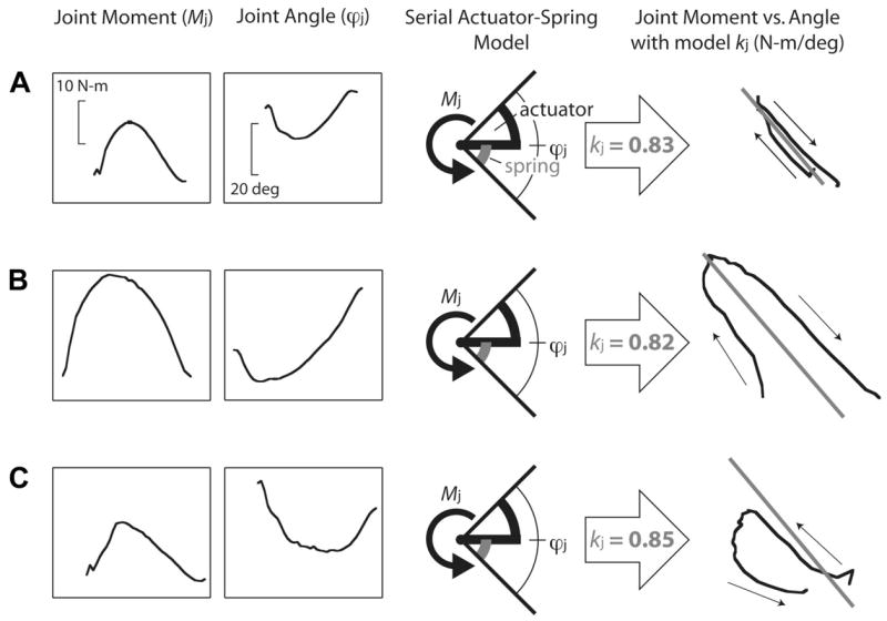
Examples of kinetics and kinematics of the ankle during level (A), uphill (B), and downhill running (C). The joint moment M_j and joint angle ϕ_j are inputs to the serial actuator-spring model for a joint. The model imposes the experimental moment and constrains the combined deflection of the spring (gray) and actuator (black) to match the experimental joint angle. The spring constant requiring the least actuator work is found iteratively. Superimposed on plots of joint moment vs. angle, the modeled spring constant (gray line) resembles a regression through the level data (A) but not the uphill (B) or downhill (C) data. Arrows on the moment-angle plots represent time progression; hence, the uphill work loop indicates positive work and the downhill work loop indicates negative work.

Because the actuator and spring are in series, they are subjected to the same moment, the joint moment M_j. Work depends on moment and angular deflection; hence, with an infinitely stiff spring, actuator and joint work will be equal (Fig. 3). The opposite case is that in which spring deflection is sufficient to match the experimentally measured joint deflection: the actuator does not deflect and does zero work (Fig. 3). Net work (W) is determined by the numerical integration of power, in this example the product of M_j and angular velocity of the joint (ω_j) or actuator (ω_a), over t_c. Hence, the net work of a joint during a footfall is

Fig. 3.

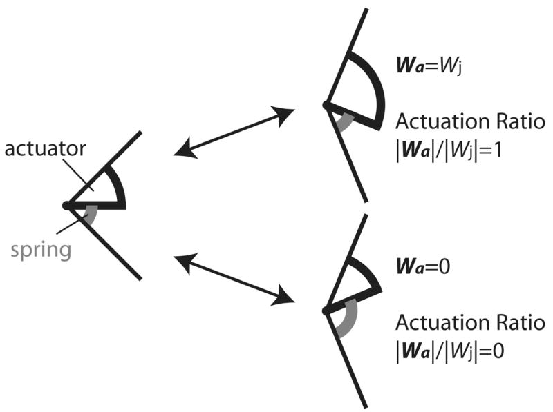
The serial actuator-spring model partitions overall joint deflection into spring (gray lines) and actuator (black lines) deflection. Functional extrema are represented by only actuator deflection [actuation ratio (AR) = 1] or only spring deflection (AR = 0). W_a and W_j are net actuator work and net joint work, respectively; |W_a|and |W_j|are total actuator work and total joint work, respectively.

$$W_{\text{j}}=\int (M_{\text{j}}\times {\omega }_{\text{j}})\text{d}t$$ (3)

and actuator net work is

$$W_{\text{ja}}=\int (M_{\text{j}}\times {\omega }_{\text{a}})\text{d}t$$ (4)

Likewise, net work of the radial leg is

$$W_{\text{r}}=\int (F_{\text{r}}\times V_{\text{r}})\text{d}t$$ (5)

and actuator net work is

$$W_{\text{ra}}=\int (F_{\text{r}}\times V_{\text{a}})\text{d}t$$ (6)

The total work |W|for a given joint or leg is determined by numerical integration of the absolute value of power over t_c, such that the integrated quantities in Eqs. 3–6 are replaced with their absolute values. In other words, the magnitudes of positive and negative work are summed to yield |W|.

For a given joint, the dimensionless actuation ratio (AR) is the ratio of total actuator to total joint work:

$$\text{AR}=\mid W_{\text{a}}\mid /\mid W_{\text{j}}\mid$$ (7)

and, for a leg,

$$\text{AR}=\mid W_{\text{a}}\mid /\mid W_{\text{r}}\mid$$ (8)

By varying k, minimum AR was determined iteratively for each trial of a given joint or leg. AR is between 0 (i.e., pure compliance) and 1 (i.e., pure actuation), as illustrated in Fig. 3. The optimal k is that which minimizes actuator work and, hence, AR. Using the least-squares regression slope of M_j on ϕ_j (°), or F_r on L_r, in the leg, as an initial estimate of k, a range of ±10⁵ values were tried at intervals of 0.001 N·m/deg (or 0.001 kN/m, in the leg) to iteratively determine the k that minimized AR.

SNW is the absolute value of the ratio of net work to total work in a joint or leg:

$$\text{SNW}=\mid W_{\text{j}}/\mid W_{\text{j}}\mid \mid$$ (9)

for a joint and SNW

$$\text{SNW}=\mid W_{\text{r}}/\mid W_{\text{r}}\mid \mid$$ (10)

for a leg. Unlike AR, SNW depends only on measured joint or leg mechanics, not the serial actuator-spring model. SNW is distinct in that it quantifies net work with regard to total work. For example, W may increase in direct proportion to |W|, such that net work increases in a given joint or leg while SNW, the basic mechanical behavior, of the joint or leg is unchanged. In this report, we will describe changes in SNW of a given joint or leg as specific work modulation to avoid confusion with work modulation, which commonly describes changes in net work.

Statistical methods

A three-way ANOVA with subject, slope (level, up, or down), and gait (trot or gallop) was used to assess experimental and model parameters. Tukey’s honestly significant difference (THSD) post hoc tests were used in slope and gait comparisons (Systat 10.2). Differences were considered significant if P ≤ 0.05. Unless otherwise noted, reported values are least squares means ± SE.

RESULTS

Footfall parameters

Mean forward velocity was significantly greater during galloping than trotting (forelimb trial, 3.00 ± 0.08 vs. 2.30 ± 0.07 ms⁻¹; hindlimb trial, 2.90 ± 0.09 vs. 1.90 ± 0.09 ms⁻¹) and greater during level than both up-and downhill running (Table 2). Consistent with faster locomotion, mean resultant GRF was significantly greater during galloping than trotting (forelimb, 225 ± 4.4 vs. 199 ± 5.2 N; hindlimb, 133 ± 2.8 vs. 113 ± 2.9 N). Load redistribution to the “downslope” limb was a prominent effect when comparing up- and downhill with level running (Table 2). Forelimb resultant GRF was greatly reduced on the uphill with respect to level and downhill, whereas that of the hindlimb was greatly reduced on the downhill with respect to level and uphill. The angle of the resultant GRF (θ; Eq. 1) was statistically similar in galloping vs. trotting (forelimb, −4.40 ± 0.56 vs. −5.40 ± 0.65°; hindlimb, −0.130 ± 0.77 vs. 0.110 ± 0.78°). Grade, on the other hand, strongly influenced θ of the fore- and hindlimb, with significantly increased (i.e., propulsive) angles during uphill running and significantly decreased (i.e., braking) angles during downhill running (Table 2). Although footfall parameters reveal several differences between trotting and galloping, such gait-specific differences are the exception when considering mechanical characteristics of the individual joint and leg. Of the 12 functional parameters considered for each limb, only one in the forelimb (radial leg SNW) and two in the hindlimb [ankle AR and metatarsophalangeal joint (MTP) SNW] showed significant differences (indicating lesser values at the gallop in each case).

Table 2.

Forelimb and hindlimb footfall parameters

	n	v̄, m/s	P ≤ 0.05	θ,°	P ≤ 0.05	F̄, N	P ≤ 0.05
Forelimb
Level	45	3.2 ± 0.07	U,D	−4.5 ± 0.59	U,D	256 ± 4.6	U,D
Uphill	22	2.4 ± 0.10	L	−.5 ± 0.84	L,D	152 ± 6.6	L,D
Downhill	23	2.3 ± 0.10	L	−17.7 ± 30.81	L,U	228 ± 6.4	L,U
Hindlimb
Level	32	2.9 ± 0.10	U,D	1.8 ± 0.85	U,D	140 ± 3.1	D
Uphill	20	2.1 ± 0.12	L	16.6 ± 1.1	L,D	138 ± 3.9	D
Downhill	25	2.2 ± 0.11	L	−18.4 ± 0.97	L,U	90 ± 3.6	L,U

L, U, and D indicate significant difference from level, uphill, and downhill parameters, respectively.

Serial actuator-spring model: foreleg

Of the forelimb joints modeled, only the distal metacarpophalangeal joint (MCP) showed substantial spring character as evidenced by AR < 0.5 during level and AR < 0.6 during up- and downhill running (Fig. 4A). The wrist showed some spring character during level running (AR = 0.64) but primarily actuation (AR ~ 0.8) during up- and downhill running. Regardless of slope, the elbow was mostly actuated (AR ~ 0.8). The radial foreleg model showed greater spring character than any individual joint during level (AR = 0.37) and downhill (AR = 0.51) running (Fig. 4A). Radial actuation was more prominent during uphill (AR = 0.65) compared with level and downhill running but still intermediate with respect to the individual joints. During up- and downhill compared with level running, the individual joints (except elbow) and radial foreleg showed significantly increased AR, indicating more actuator contribution.

Fig. 4.

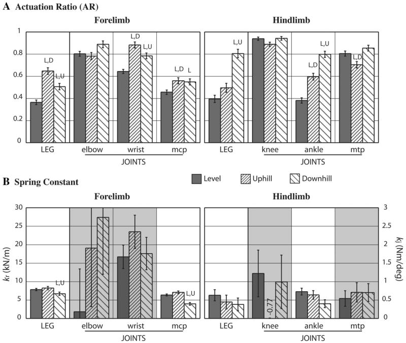
ARs (A) and spring constants (B) for the radial leg and 3 leg joints of the forelimb and hindlimb. Values from level, uphill, and downhill running are shown with SE bars. Significant difference (P < 0.05) from level, uphill, or downhill values is indicated, respectively, by L, U, or D. Background shading in B indicates AR > 0.6 during level running.

The serial actuator-spring model determined spring constants for each joint and for the radial foreleg. Substantial variability in the elbow and wrist suggests little functional relevance of the spring constant to these joints (Fig. 4B). In contrast, the spring constant of the MCP was consistent in level (k_j = 0.64 N·m/deg) and uphill (k_j = 0.71 N·m/deg) but significantly reduced during downhill (k_j = 0.40 N·m/deg) running. This pattern was repeated in the radial foreleg spring constant during level (k_r = 7.8 kN/m), uphill (k_r = 8.2 kN/m), and downhill (k_r = 6.7 kN/m) running. Hence, the MCP appears to most strongly influence overall patterns of foreleg compliance.

Serial actuator-spring model: hindleg

Of the hindlimb joints, only the ankle showed substantial spring character. The knee (AR ~ 0.9) and MTP (AR ~ 0.8) were largely actuated across level and slope running conditions (Fig. 4A). The ankle actuator contribution varied significantly across level (AR = 0.38), uphill (AR = 0.60), and downhill (AR = 0.80) running. This pronounced pattern across slope conditions is reflected in the radial hindleg AR (0.40, 0.50, and 0.80, respectively), indicating substantial influence of the ankle on overall hindleg spring character (Fig. 4). In contrast to the ankle, the knee and MTP showed little or no change in AR across slope conditions.

As in the elbow, spring constants of the primarily actuated knee were highly variable and of no functional importance. In the actuation-dominated MTP, however, the model produced consistent spring constants similar in magnitude to those of the MCP but with much greater SEs (Fig. 4B). Ankle spring constants were statistically similar (P < 0.05) during level (k_j = 0.73 N·m/deg), uphill (k_j = 0.64 N·m/deg) and downhill (k_j = 0.40 N·m/deg) running. These are also in the same range as the MCP spring constants. Radial hindleg spring constants (level, k_r = 6.3 kN/m; uphill, k_r = 4.5 kN/m; and downhill, k_r = 3.8 kN/m) are notably reduced, however, compared with those of the foreleg (Fig. 4B). Although ankle and radial hindleg spring constants are both statistically similar across slope conditions, the reduction in these spring constants during downhill running resembles the significant reduction in MCP and radial foreleg spring constants during downhill running (Fig. 4B).

Net work and SNW: foreleg

The elbow did the greatest positive net work during uphill and negative net work during downhill running compared with the more distal foreleg joints. Yet the elbow did very little net work during level running, so these changes represent statistically significant work modulation between slope conditions (Fig. 5A). Furthermore, SNW at least doubled during uphill (SNW = 0.56) and downhill (SNW = 0.52) with respect to level (SNW = 0.26), indicating changes in joint mechanical behavior (i.e., specific work modulation; Fig. 5B). Net work of the radial foreleg followed the elbow’s pattern of work modulation but with a positive offset, such that net work was substantially positive during level and nearly zero during downhill running (Fig. 5A). Changes in radial foreleg SNW were also statistically significant across level (SNW = 0.15), uphill (SNW = 0.56), and downhill (SNW = 0.31), indicating a twofold increase in specific work modulation during downhill and more than a fourfold increase during uphill, compared with level running (Fig. 5B).

Fig. 5.

Net work (A) and specific net work (SNW; B) for the radial leg and 3 leg joints of the forelimb and hindlimb. Values from level, uphill, and downhill running are shown with SE bars. Significant difference (P < 0.05) from level, uphill, or downhill values is indicated, respectively, by L, U, or D.

In contrast to the elbow, the wrist did minimal net work under all slope conditions and maintained SNW ~0.20 (Fig. 5). Surprisingly, the MCP did substantial negative net work during level running but only slight negative net work during uphill and slight positive net work during downhill running. Accordingly, SNW of the MCP was greatest during level (SNW = 0.37), intermediate during uphill (SNW = 0.24), and least during downhill (SNW = 0.15) (Fig. 5B). These changes in MCP net work and SNW with slope are statistically significant and represent modulation of energy absorption.

Net work and SNW: hindleg

Of the hindleg joints, both the knee and ankle contribute significantly greater positive net work during uphill running, and greater negative net work during downhill compared with level running. Although both joints show significant work modulation across grade, the ankle contributes much more positive work and the knee contributes more negative work (Fig. 5A). The knee also shows increased SNW during downhill (SNW = 0.82) but not during uphill (SNW = 0.48) compared with level (SNW = 0.61) running; hence, specific work modulation occurs only during downhill running in the knee (Fig. 5B). Despite significant changes in net work at the ankle, SNW is statistically similar across level (SNW = 0.52), uphill (SNW = 0.55), and downhill (SNW = 0.61) conditions, showing no specific work modulation at the ankle. In other words, the ankle does net positive and negative work without changing its basic mechanical behavior (i.e., SNW). The radial hindleg does some negative net work during level, positive net work during uphill, and substantial negative net work during downhill running (Fig. 5A). These changes across grade are significant and indicate work modulation by the hindleg. Radial hindleg SNW follows a pattern strikingly similar to that of the foreleg: level (SNW = 0.27), uphill (SNW = 0.58), and downhill (SNW = 0.38), indicating significantly greater specific work modulation during uphill than downhill running (Fig. 5B). As in the MCP, the MTP was variably absorptive, but did nearly zero net work during downhill running. In contrast to the MCP pattern, more negative net work was done during uphill than level running (Fig. 5A). Due to extremely reduced MTP total work, SNW was greater during downhill running than level and uphill running (Fig. 5B).

DISCUSSION

Biological implications and robotic applications

The serial actuator-spring model, along with net work and SNW analyses, can be used to characterize the function of individual joints and of the radial leg during running. Here, we differentiate level, uphill, and downhill running, but these techniques might also prove useful in comparisons between species, as well as across different locomotor tasks. In addition, this approach yields basic principles of leg and joint mechanics that can be transferred to running machines. Despite vast differences in leg design and actuator characteristics, legged robots can employ four main findings of this report: 1) radial leg spring constants, 2) proximal joint actuation, 3) distal joint compliance, and 4) distal joint energy absorption. Regardless of leg design, radial leg spring constants measured in animals may be applied to running machines of similar mass and leg number. Here, fore- and hindleg radial spring constants ranged from 6 to 8 kN/m and from 4 to 6 kN/m, respectively. From an engineering perspective and as evidenced by living animals, proximal placement of massive actuators (or muscles) greatly reduces rotational inertia of the leg, thus reducing limb retraction and protraction moments and energetic cost required to swing the leg fore and aft (31, 41). By contrast, compliance can be provided by long, thin tendons that descend to the foot, adding little mass to the distal leg. This is the case in the foreleg (MCP compliance) and the hindleg, although the MTP is substantially damped. As discussed by Alexander (1), springs function not only to reduce the energetic cost of locomotion but to reduce impact loading and prevent chatter of the foot on the ground. Damping at the distal joints, as suggested here by energy absorption at the MCP and MTP, would also reduce chatter. Hence, distal compliance and energy dissipation “soften” the interaction of the more actuated proximal limb with the substrate. This strategy seems effective for meeting the challenges of an irregular natural environment, which are quite extreme in the mountainous terrain inhabited by goats.

Running speed

Level running speeds were greater than up-and downhill speeds in the trotting and galloping trials analyzed in this report (Table 2). These are comparable to the speeds chosen by slightly larger dogs (body mass of 30 kg) trotting on the level (3.1 ms ^{− 1}) vs. up (2.2 ms⁻¹) and down (2.6 ms⁻¹) a 15° grade (25, 27). Hence, reduced running speeds appear to be typical of grade running in quadrupeds the size of goats and dogs. Horses have also been shown to trot more slowly on a 6° incline (4.4 ms⁻¹) than on the level (5.1 ms⁻¹) (42). As might be expected, level running speed in our combined trotting and galloping trials approximates the trot-gallop transition speed predicted for quadrupeds of this size (3.1 ms⁻¹), given an average body mass of 24 kg for our subjects, by the allometric equation of Heglund and Taylor (20).

Force distribution

A second characteristic of slope running is redistribution of GRF to the downslope limbs, either fore- or hindlimbs depending upon the direction of travel. By measuring simultaneous footfalls of trotting dogs, the distribution of normal GRF has previously been determined within a trotting step by the fraction of forelimb to total normal impulse: level (0.65), uphill (0.52), and downhill (0.70) (25, 27). As assessed from multiple steps on a single force platform, horses show a less extreme redistribution of load during 6° incline trotting: 0.57 on the level to 0.52 on the incline (10). In the present study, simultaneous individual footfall forces are not measured, and trotting and galloping are considered together. Nonetheless, computing the mean normal GRF,

$$F_{\text{n}}=\overline{\mathbf{F}}\times cos\theta$$ (11)

using values from Table 2, the ratio of mean forelimb to the sum of mean fore- and hindlimb normal GRF yields strikingly similar ratios: level (0.65), uphill (0.53), downhill (0.72). Hence, forelimb-hindlimb normal load redistribution associated with 15° grade running is quite comparable in dogs and goats.

Force angle

A dimensionless indicator of limb function during level and slope running is the angle θ of the mean resultant GRF during the footfall (computed as the angle of the impulse, Eq. 1). This angle has been assessed previously for both single-limb and multiple-limb resultant GRF impulse of trotting dogs (25, 27). Resultant GRF impulse angle has also been examined in birds during running perturbations (8), and peak resultant GRF angle has been used to characterize human running during gravitational and inertial manipulations (6). In dogs, fore- and hindlimb resultant GRF angles are, respectively, −3.3/5.8° (level), 11.8/18.4° (uphill), and −18.0/−7.7° (downhill). These steady-speed angles are generally more positive than the angles observed here in goats running on the same grade: −4.5/1.8° (level), 7.5/16.6° (uphill), and −17.7/−18.4° (downhill). From Table 2, the mean shear component of GRF can be determined by

$$F_{\text{n}}=\overline{\mathbf{F}}\times sin\theta$$ (12)

Summing the fore- and hindlimb mean shear components, then dividing by the sum of fore- and hindlimb mean resultant GRF magnitudes and taking the inverse sine, reveals a braking bias of the GRF resultant under each condition: −2.3° on the level and (with respect to the 15° grade) −3.0° uphill and −3.5° downhill. Hence, our sample of footfalls represents slight and reasonably consistent net braking across grade conditions.

Actuator-spring model of the radial leg

When modeled as a radial actuator and spring in series, as introduced in this report, the fore- and hindleg of running goats show at least as much springlike character as any individual joint. During level running, in particular, compliance is substantial, with AR < 0.4 in both the fore- and hindleg. The corresponding spring constants are 7.8 kN/m (foreleg) and 6.3 kN/m (hindleg). Hence, the foreleg is somewhat stiffer than the hindleg. Radial spring constants are relatively consistent across grade with the exception of a significant reduction in foreleg spring constant during downhill running. Since this closely mirrors changes in the MCP spring constant, it will be addressed in the discussion of distal joints.

Across grade conditions, the whole leg AR tracks that of the principal joint spring, as can be seen by comparing foreleg to MCP AR and hindleg to ankle AR (Fig. 4A). From a minimum AR during level running of ~0.4, values climb to between 0.5 and 0.8 during grade running, indicating an expected increase in actuation due to net work requirements of grade running. Given the forelimb braking bias and hindlimb propulsive bias of quadrupedal runners (27), one might predict greater foreleg actuation during downhill and greater hindleg actuation during uphill running. Surprisingly, the opposite is observed: foreleg AR increases more during uphill and hindleg AR increases more during downhill running. In the following sections, consideration of whole limb work helps to resolve this seemingly contradictory finding.

Work characteristics of the radial leg

In accordance with radial leg AR patterns, the foreleg does greater positive net work during uphill running and the hindleg does greater negative net work during downhill running (Fig. 5A). This does not, however, represent net work of the entire limb. Here, the distinction between leg and limb is functionally, as well as anatomically, important. The radial work done by the leg comprises all of the work done by individual joints between the proximal joint (i.e., shoulder or hip) and foot. These joints flex or extend to shorten or lengthen the leg radially. In addition, the proximal joint itself may contribute some but not necessarily all of its work to shortening or lengthening of the leg. This quantity of proximal joint work was not measured directly in our analysis. Instead, the additional leg joint work is apparent in the difference between the sum of the individual joint and radial leg net work in Fig. 5A. Note that foreleg net work is consistently greater than the sum of individual joint net work. Similarly, hindleg net work is consistently less than sum of individual joint net work. This indicates, respectively, a positive and negative proximal joint contribution to the net work of the radial leg.

While radial work is achieved by positive or negative thrust in line with the leg, proximal joints may also do work to retract the leg during stance; this is termed “lever” function by Gray (16). To achieve forward locomotion, the legs must be retracted at an appropriate angular velocity so that the trunk passes over the fixed foot position during stance. Using high-speed x-ray video of small mammals, Fischer and coworkers (14) confirmed that foreleg retraction occurs primarily about the scapula, and hindleg retraction occurs primarily about the hip joint. In the absence of a retracting or protracting moment, no work is done during leg retraction. Such a scenario may be plausible during level running, but lever function appears to play a role in downhill and, especially, uphill trotting of dogs (25).

SNW is a dimensionless number designed to characterize the mechanical behavior of individual joints, but it applies equally well to the radial leg. Foreleg and hindleg radial SNW show a strikingly similar pattern across grade running conditions (Fig. 5A). Lower SNW during level running in the hindleg (0.27) and, especially, in the foreleg (0.15), indicate conservative leg mechanics and reflect greater hindleg vs. foreleg individual joint SNW. During uphill running, SNW is nearly 0.6, indicating that net work approaches 60% of total work. During downhill running, SNW increases less dramatically to between 0.3 and 0.4. Hence, radial leg mechanics are more-or-less conservative during level running, but net work is modulated increasingly during downhill and uphill running. The individual joints that contribute to this work modulation are discussed in following sections.

Whole limb work

The work contributed by the hip and shoulder (scapulohumeral joint) may be augmented by the limb girdles that link them to the trunk (14, 22). It is this complete structure, limb girdle plus leg, that defines the anatomic limb and contributes to the total work done on the center of mass. Net work of the hip itself has been reported to be moderately positive in dogs running on the level, which more than offsets the net negative work of distal leg joints (18). When required for tasks such as uphill running and jumping, a great deal of positive hindlimb work can be done by the massive hip extensors, which act to retract the hindleg (33, 34). Compared with level running, greater recruitment and shortening of a principal hip extensor, biceps femoris, has been observed in rats ascending a 15° incline (15). The pelvis may also rotate with respect to the spine, and, especially during galloping, the lumbar spine may even ventroflex to do work on the center of mass (16).

Previous measurements of shoulder (scapulohumeral) joint work in running dogs indicate very modest positive net work (18). This is consistent with the observation that the forelimb generally retracts about a point on the more proximal scapula rather than the shoulder itself (14, 16, 22). A well-developed muscular sling binds the scapula and proximal humerus to the thorax (see Refs. 23 and 39), and because of this muscular rather than bony attachment, it is possible for the shoulder girdle to do work by exerting force in line with the leg, as well as by lever action. In the muscular sling, the large, fan-shaped serratus ventralis thoracis has been shown to be most important for weight support and to be more strongly recruited during 14° downhill than during level running of dogs (5). The authors explain that this increased recruitment is associated with redistribution of weight support to the forelimb; however, it is also consistent with increased energy absorption by active lengthening of this muscle to meet the negative work requirements of downhill running. Based on their anatomic positions, several shoulder girdle muscles may act as protractors (34), possibly contributing to forelimb negative work during stance.

Given that whole limb work depends on limb girdle work, proximal joint (lever) work and radial leg work, it is useful to compare radial leg net work to the total net work done on the center of mass by the limb. Net work of the limb can be estimated by multiplying the shear component of mean force (Eq. 12) by the shear mean velocity (Table 2) and the time of contact. Given mean forelimb contact times of 0.10 s (level), 0.14 s (uphill), and 0.13 s (downhill), this yields −6.4 J (level), 6.7 J (uphill), and −21.0 J (downhill). Given mean hindlimb contact times of 0.11 s (level), 0.16 s (uphill), and 0.14 s (downhill), this yields 1.4 J (level), 13.2 J (uphill), and −8.7 J (downhill). Radial leg net work (Fig. 5A) is actually opposite in sign to total limb net work during level running. In other words, the radial foreleg is generative and the radial hindleg is absorptive, despite the negative net work of the forelimb and the positive net work of the hindlimb on the center of mass. Given that the whole forelimb does negative net work during level running, the shoulder girdle and scapulohumeral joint must absorb the energy generated by the radial foreleg (2.7 J) plus an additional 6.4 J. Conversely, the pelvic girdle and hip must generate the energy absorbed by the radial hindleg (2.2 J) plus an additional 1.4 J. The sum of forelimb and hindlimb net work (−5.0 J) is associated with net braking in our sample of level running footfalls. It should also be cautioned that the total limb work discussed here is an estimate based on mean shear force of a given limb and mean shear velocity of the CoM, not the time-integrand of limb power, as defined by the individual limbs method of Donelan et al. (9).

The generative tendency of the radial foreleg increases during uphill running, and the absorptive tendency of the radial hindleg increases during downhill running. Given the overall braking bias of the whole forelimb and propulsive bias of the whole hindlimb, this is somewhat unexpected. Such a work pattern in the radial fore- and hindleg is likely associated with elbow-back, knee-forward leg geometry, in that the elbow moment tends to increase as the GRF vector becomes more propulsive and the knee moment tends to increase as the GRF vector becomes more braking. Thus elbow-back geometry is conducive to positive work, and knee-forward geometry is conducive to negative work of the radial leg. The radial leg contributes 84% of forelimb net (positive) work during uphill running, but only 2% of forelimb net work (negative) during downhill running. Conversely, the radial leg contributes 87% of hindlimb net work (negative) during downhill running, but only 30% of hindlimb net work (positive) during uphill running. Hence, the radial foreleg accounts for most of the forelimb positive work during uphill running and the radial hindleg accounts for most of the hindlimb negative work during downhill running, whereas the radial leg contributes minimally to forelimb negative work during downhill running and hindlimb positive work during uphill running. In these cases, the proximal joint and limb girdle contribute the majority of work.

Proximal leg joints: elbow and knee

In agreement with anatomically based predictions, the serial actuator-spring model identifies the more proximal elbow and knee as actuated joints with little or no spring character (i.e., AR ~ 0.8 or greater). This is consistent across grade conditions, suggesting that the muscle-tendon systems spanning these joints have little intrinsic compliance. The elbow and knee extensor muscles of the goat are substantial and their tendons are, in fact, short and thick (7).

Consistent with muscle-tendon architecture, the elbow does the greatest positive net work of any foreleg joint during uphill running and the greatest negative net work during downhill running. The knee also does the greatest negative net work of any hindleg joint during downhill running but the ankle does the greatest positive net work during uphill running (Fig. 5A). Sustained, active lengthening in a major knee extensor, vastus lateralis, of rats during descent of a 15° grade (15) strongly supports the observed strutlike braking function of the hindleg facilitated by the action of proximal muscles about the knee.

Although not as straightforward as the foreleg pattern, there is a well-established anatomic explanation for the sharing of net work between the knee and ankle. As depicted in Fig. 1, the ankle extensor crosses the knee, linking knee extension and ankle extension. On the basis of this kinematic linkage, Gregersen and Carrier (17) estimate that 41% of positive ankle work is energy transferred from the knee to ankle during jumping in dogs. Mechanical energy transfer between knee and ankle has also been assessed during level locomotion of quadrupeds (18, 35, 36).

Given that complex, multijoint muscle-tendon systems can transfer energy between joints, how can modulation of work be ascribed to one joint or another? Here, we address this issue by using SNW to identify the mechanical behavior of individual joints. Specific work modulation refers to changes in SNW to accommodate various locomotor demands. In the knee, SNW increases significantly during downhill compared with level running (Fig. 5B), indicating that the knee is less conservative as it absorbs energy downhill. Likewise, SNW increases in the elbow during both uphill and downhill compared with level running, indicating less conservative mechanics as the elbow generates or absorbs energy to accommodate the grade. In agreement with anatomic predictions, the knee and elbow show specific work modulation during uphill and downhill running.

Intermediate leg joints: wrist and ankle

In contrast to the more proximal elbow and knee, the wrist shows at least slight spring function, while the ankle is clearly the principal hindleg spring. Considering level and grade conditions together, AR is in the expected range for the intermediate proximodistal position of these joints (Fig. 4A). The ankle during level running, however, shows even more spring character than expected, with AR ~ 0.4. Nonetheless, ankle AR increases to ~0.6 uphill and to ~0.8 downhill, indicating distinctly increased actuation during grade running. Despite these differences in AR, the ankle’s spring constant (optimized by minimization of AR) was statistically unchanged across level and grade conditions. This similarity reflects the intrinsic compliance of the common calcaneal (i.e., Achilles) tendon on which the ankle extensor muscles pull. During downhill running, the nearly significant (P = 0.079) decrease of ankle spring constant suggests a possibility of spring constant modulation, perhaps by variable recruitment of parallel muscle systems, engaging or disengaging their aponeurotic connections to the calcaneal tendon.

The wrist does minimal net work across level and grade running conditions. In contrast, the ankle does the greatest positive net work of any hindleg joint during uphill and also does substantial negative net work during downhill running (Fig. 5A). As already discussed, it has been estimated that as much as a one-half of the work at the ankle may be due to energy transferred from the knee. Hence, the net work done at the ankle is not necessarily done by the ankle extensor muscles themselves. Results of in vivo measurements from the primary ankle extensors of goats, lateral and medial gastrocnemius and superficial digital flexor, show that these muscles do very little (−0.26 to 7.46 J/kg) net work during uphill or downhill (15°) running of goats (29).

In contrast to the elbow and knee, which show specific work modulation on grades, there is no change in SNW of the wrist or ankle (Fig. 5B). This is expected in the case of the wrist, which does virtually no net work in any grade condition, but would seem unlikely for the ankle, which does substantial net work. Given that the ankle SNW (net work/total work) indicates equally conservative mechanics across level and grade conditions, net positive (uphill) and negative (downhill) work done at the ankle must be accompanied by proportionate increases in total work. For example, calcaneal tendon tension would be greater under the greater ankle moments required during uphill running. Hence, the tendon would be stretched more, increasing negative along with positive work, and thus increasing total joint work. In other words, this is a direct consequence of actuating a joint via a compliant tendon in-series with the muscle. These findings are consistent with direct in vivo measurements of ankle extensor tendon forces recorded for level vs. incline conditions, which showed a 1.4-to 2.5-fold increase in force during 15° incline trotting (29). Although ankle mechanics show equal SNW in level vs. grade conditions, it is important to note that they are not equally springlike, as evidenced by AR (Fig. 4A), which is subject to the temporal relationship between joint moment and joint angle (e.g., Fig. 2).

Distal leg joints: MCP and MTP

Considering the most distal leg joints, the MCP is clearly the principal spring of the foreleg (AR between 0.4 and 0.6), but the MTP shows much less spring character (AR ~ 0.8) than the more proximal ankle (Fig. 4A). The MCP agrees with the basic anatomic prediction that distal joints supported by long tendons will behave as springs. Thus it is surprising that the MTP shows little spring character in spite of its distal position. Despite these differences, spring constants are quite similar in the MCP and MTP (Fig. 4B). They are, in fact, in the same range as ankle spring constants (~0.5 N·m/deg). The MCP spring constant decreases significantly during downhill running, reflecting the nonsignificant pattern seen in the ankle spring constant. A comparison of in vivo and in vitro MCP spring constants in horses suggests a minimal influence of muscle activation (28). Nonetheless, the presence of parallel muscle-tendon systems indicates the potential for spring constant modulation, which may be more prominent in smaller quadrupeds with less restrictive muscle-tendon architectures.

Both the MCP and MTP do substantial negative net work during level running. More surprisingly, they do negative net work during uphill running, while neither joint does much net work during downhill running (Fig. 5A). Hence, the MCP and MTP absorb energy during level and uphill running but not during downhill running, where they could potentially contribute to the required negative work. The dissipative capacity of the MCP and MTP appears to be compromised by decreased joint moments during downhill running (i.e., to less than one-half of the level moment; Table 3). This is attributable not only to decreased GRF (Table 2) but also to significantly decreased lever arms of the GRF about these joints (Table 3), indicating a closer alignment of the GRF vector with the joint during downhill braking. Hence, requirements for substantial energy absorption (i.e., braking) fall to the more proximal joints and limb girdle, particularly during downhill running.

Table 3.

Mean joint moment, mean joint angle, and joint angular excursion of fore- and hindlimb joints

Level	M̄j, m/s	P ≤ 0.05	ϕ̄j,°	P ≤ 0.05	ϕj,max − ϕj,min,°	P ≤ 0.05
Level
Forelimb joint
Elbow	4.6 ± 0.3	D	151.4 ± 0.7	U,D	23.7 ± 0.5	U
Wrist	7.1 ± 0.3	U,D	177.0 ± 0.5	U,D	15.1 ± 0.5	D
MCP	7.0 ± 0.2	U,D	151.4 ± 0.6	U,D	24.9 ± 0.5	U,D
Hindlimb joint
Hip	6.8 ± 0.72	U,D	99.4 ± 1.1		16.8 ± 0.7	U
Knee	0.73 ± 0.56	U,D	134.7 ± 1.3	U	19.0 ± 0.7	D
Ankle	7.7 ± 0.35	U,D	147.6 ± 0.8	U	26.9 ± 0.8	U,D
MTP	4.4 ± 0.20	U,D	156.2 ± 0.8		20.7 ± 0.7	U,D
Uphill
Forelimb joint
Elbow	5.5 ± 0.7	D	146.7 ± 2.0	L	31.3 ± 1.5	L,D
Wrist	5.3 ± 0.4	L,D	180.2 ± 0.9	L,D	17.5 ± 0.9	D
MCP	5.0 ± 0.3	L,D	160.5 ± 0.6	L	20.9 ± 1.4	L
Hindlimb joint
Hip	15.0 ± 1.2	L,D	102.8 ± 1.2	D	22.1 ± 1.5	L,D
Knee	33.8 ± 0.70	L,D	124.4 ± 1.8	L,D	19.5 ± 1.3	D
Ankle	12.1 ± 0.95	L,D	138.9 ± 2.6	L	42.2 ± 2.4	L,D
MTP	7.2 ± 0.50	L,D	154.1 ± 0.8		26.1 ± 1.8	L,D
Downhill
Forelimb joint
Elbow	0.8 ± 0.7	L,U	142.9 ± 1.5	L	26.2 ± 1.5	U
Wrist	3.7 ± 0.3	L,U	173.8 ± 0.6	L,U	35.0 ± 2.5	L,U
MCP	2.8 ± 0.3	L,U	162.4 ± 1.5	L	19.2 ± 2.0	L
Hindlimb joint
Hip	30.6 ± 0.71	L,U	98.2 ± 1.0	U	13.9 ± 1.3	U
Knee	4.1 ± 0.44	L,U	131.6 ± 2.1	U	37.6 ± 2.8	L,U
Ankle	3.2 ± 0.43	L,U	142.0 ± 32.6		31.8 ± 1.8	L,U
MTP	2.0 ± 0.24	L,U	157.1 ± 0.7		14.1 ± 0.7	L,U

M̄_j, mean joint moment; ϕ¯_j, mean joint angle; ϕ_j,max, maximum ϕ_j; ϕ_j,min, minimum ϕ_j; ϕ_j,max − ϕ_j,min, joint angular excursion. L, U, and D indicate significant difference from level, uphill, and downhill parameters, respectively.

Conclusions

During level running, the radial foreleg and hindleg show as much spring character as any individual joint and are increasingly actuated to accommodate grade running. The radial foreleg tends to be generative and the radial hindleg tends to be absorptive. This contrasts with the overall function of the forelimb to provide negative work and the hindlimb, positive work. Yet the radial foreleg contributes substantially to forelimb positive net work during uphill running and the radial hindleg to hindlimb negative net work during downhill running. In accordance with anatomic predictions, the principal foreleg joint spring is the MCP. However, the principal hindleg joint spring is the ankle, which is proximal to the MTP. This suggests that compliance is largely due to the digital flexor tendons and the common calcaneal tendon. Proximal leg joints, the elbow and knee, tend to do the greatest net work and show substantial specific work modulation to accommodate grade conditions. The wrist does virtually zero net work, but the ankle does some negative net work during downhill, and a great deal of positive net work during uphill, running. Despite its work contribution, the ankle shows no specific work modulation across grade, an observation consistent with its springlike function and with the transfer of energy between knee and ankle. Distal joints, the MCP and MTP, tend to absorb energy during level and uphill, but do little net work during downhill running, requiring energy absorption at more proximal joints.

References

- 1.Alexander RM. Three uses for springs in legged locomotion. Int J Robot Res. 1990;3:37– 48. [Google Scholar]
- 2.Arampatzis A, Brüggemann GP, Metzler V. The effect of speed on leg stiffness and joint kinetics in human running. J Biomech. 1999;32:1349–1353. doi: 10.1016/s0021-9290(99)00133-5. [DOI] [PubMed] [Google Scholar]
- 3.Bertram JEA, Lee DV, Todhunter RJ, Foels WS, Williams A, Lust G. Multiple force platform analysis of the canine trot: a new approach to assessing basic characteristics of locomotion. Vet Comp Orthoped Traumatol. 1997;10:160–169. [Google Scholar]
- 4.Blickhan R, Full RJ. Similarity in multilegged locomotion—bouncing like a monopode. J Comp Physiol A. 1993;173:509–517. [Google Scholar]
- 5.Carrier DR, Deban SM, Fischbein T. Locomotor function of the pectoral girdle “muscular sling” in trotting dogs. J Exp Biol. 2006;209:2224–2237. doi: 10.1242/jeb.02236. [DOI] [PubMed] [Google Scholar]
- 6.Chang YH, Huang HWC, Hamerski CM, Kram R. The independent effects of gravity and inertia on running mechanics. J Exp Biol. 2000;203:229–238. doi: 10.1242/jeb.203.2.229. [DOI] [PubMed] [Google Scholar]
- 7.Constantinescu GM. Guide to Regional Ruminant Anatomy based on the Dissection of the Goat. Ames, IA: Iowa State Univ. Press; 2001. [Google Scholar]
- 8.Daley MA, Usherwood JR, Felix G, Biewener AA. Running over rough terrain: guinea fowl maintain dynamic stability despite a large unexpected change in substrate height. J Exp Biol. 2006;209:171–187. doi: 10.1242/jeb.01986. [DOI] [PubMed] [Google Scholar]
- 9.Donelan JM, Kram R, Kuo AD. Simultaneous positive and negative external mechanical work in human walking. J Biomech. 2002;35:117–124. doi: 10.1016/s0021-9290(01)00169-5. [DOI] [PubMed] [Google Scholar]
- 10.Dutto DJ, Hoyt DF, Cogger EA, Wickler SJ. Ground reaction forces in horses trotting up an incline and on the level over a range of speeds. J Exp Biol. 2004;207:3507–3514. doi: 10.1242/jeb.01171. [DOI] [PubMed] [Google Scholar]
- 11.Farley CT, Glasheen J, McMahon TA. Running springs: speed and animal size. J Exp Biol. 1993;185:71– 86. doi: 10.1242/jeb.185.1.71. [DOI] [PubMed] [Google Scholar]
- 12.Ferris DP, Liang KL, Farley CT. Runners adjust leg stiffness for their first step on a new running surface. J Biomech. 1999;32:787–794. doi: 10.1016/s0021-9290(99)00078-0. [DOI] [PubMed] [Google Scholar]
- 13.Ferris DP, Louie M, Farley CT. Running in the real world: adjusting leg stiffness for different surfaces. Proc R Soc Lond B Biol Sci. 1998;265:989–994. doi: 10.1098/rspb.1998.0388. [DOI] [PMC free article] [PubMed] [Google Scholar]
- 14.Fischer MS, Schilling N, Schmidt M, Haarhaus D, Witte H. Basic limb kinematics of small therian mammals. J Exp Biol. 2002;205:1315–1338. doi: 10.1242/jeb.205.9.1315. [DOI] [PubMed] [Google Scholar]
- 15.Gillis GB, Biewener AA. Effects of surface grade on proximal hindlimb muscle strain and activation during rat locomotion. J Appl Physiol. 2002;93:1731–1743. doi: 10.1152/japplphysiol.00489.2002. [DOI] [PubMed] [Google Scholar]
- 16.Gray J. Animal Locomotion. New York: Norton; 1968. pp. xi–479. [Google Scholar]
- 17.Gregersen CS, Carrier DR. Gear ratios at the limb joints of jumping dogs. J Biomech. 2004;37:1011–1018. doi: 10.1016/j.jbiomech.2003.11.024. [DOI] [PubMed] [Google Scholar]
- 18.Gregersen CS, Silverton NA, Carrier DR. External work and potential for elastic storage at the limb joints of running dogs. J Exp Biol. 1998;201:3197–3210. doi: 10.1242/jeb.201.23.3197. [DOI] [PubMed] [Google Scholar]
- 19.Gunther M, Blickhan R. Joint stiffness of the ankle and the knee in running. J Biomech. 2002;35:1459–1474. doi: 10.1016/s0021-9290(02)00183-5. [DOI] [PubMed] [Google Scholar]
- 20.Heglund NC, Taylor CR. Speed, stride frequency and energy cost per stride: how do they change with body size and gait? J Exp Biol. 1988;138:301–318. doi: 10.1242/jeb.138.1.301. [DOI] [PubMed] [Google Scholar]
- 21.Hildebrand M. Symmetrical gaits of horses. Science. 1965;150:701–708. doi: 10.1126/science.150.3697.701. [DOI] [PubMed] [Google Scholar]
- 22.Jenkins FA, Weijs WA. Functional anatomy of the shoulder in the Virginia opossum (Didelphis virginiana) J Zool. 1979;188:379– 410. [Google Scholar]
- 23.Kardong KV. Vertebrates—Comparative Anatomy, Function, Evolution. Boston, MA: McGraw-Hill; 1998. [Google Scholar]
- 24.Kuitunen S, Komi PV, Kyröläinen H. Knee and ankle joint stiffness in sprint running. Med Sci Sports Exerc. 2002;34:166–173. doi: 10.1097/00005768-200201000-00025. [DOI] [PubMed] [Google Scholar]
- 25.Lee DV. Mechanics of downhill and uphill running in a quadruped (Abstract). Proceedings of Annual Meeting of the Society for Integrative and Comparative Biology; 2004. [Google Scholar]
- 26.Lee DV, Bertram JEA, Todhunter RJ. Acceleration and balance in trotting dogs. J Exp Biol. 1999;202:3565–3573. doi: 10.1242/jeb.202.24.3565. [DOI] [PubMed] [Google Scholar]
- 27.Lee DV, Stakebake EF, Walter RM, Carrier DR. Effects of mass distribution on the mechanics of level trotting in dogs. J Exp Biol. 2004;207:1715–1728. doi: 10.1242/jeb.00947. [DOI] [PubMed] [Google Scholar]
- 28.McGuigan MP, Wilson AM. The effect of gait and digital flexor muscle activation on limb compliance in the forelimb of the horse Equus caballus. J Exp Biol. 2003;206:1325–1336. doi: 10.1242/jeb.00254. [DOI] [PubMed] [Google Scholar]
- 29.McGuigan MP, Biewener AA. Muscle dynamics of jumping and incline locomotion in goats (Abstract). Proceedings of the Meeting of the Society for Experimental Biology; Barcelona, Spain. 2005. [Google Scholar]
- 30.McMahon TA, Cheng GC. The mechanics of running: how does stiffness couple with speed? J Biomech. 1990;23(Suppl 1):65–78. doi: 10.1016/0021-9290(90)90042-2. [DOI] [PubMed] [Google Scholar]
- 31.Myers MJ, Steudel K. Effect of limb mass and its distribution on the energetic cost of running. J Exp Biol. 1985;116:363–373. doi: 10.1242/jeb.116.1.363. [DOI] [PubMed] [Google Scholar]
- 32.Pandy MG, Kumar V, Berme N, Waldron KJ. The dynamics of quadrupedal locomotion. J Biomech Eng. 1988;110:230–237. doi: 10.1115/1.3108436. [DOI] [PubMed] [Google Scholar]
- 33.Pasi BM, Carrier DR. Functional trade-offs in the limb muscles of dogs selected for running vs. fighting. J Evol Biol. 2003;16:324–332. doi: 10.1046/j.1420-9101.2003.00512.x. [DOI] [PubMed] [Google Scholar]
- 34.Payne RC, Veenman P, Wilson AM. The role of the extrinsic thoracic limb muscles in equine locomotion. J Anat. 2005;206:193–204. doi: 10.1111/j.1469-7580.2005.00353.x. [DOI] [PMC free article] [PubMed] [Google Scholar]
- 35.Prilutsky BI, Herzog W, Leonard T. Transfer of mechanical energy between ankle and knee joints by gastrocnemius and plantaris muscles during cat locomotion. J Biomech. 1996;29:391– 403. doi: 10.1016/0021-9290(95)00054-2. [DOI] [PubMed] [Google Scholar]
- 36.Prilutsky BI, Zatsiorsky VM. Tendon action of two-joint muscles: transfer of mechanical energy between joints during jumping, landing, and running. J Biomech. 1994;27:25–34. doi: 10.1016/0021-9290(94)90029-9. [DOI] [PubMed] [Google Scholar]
- 37.Raibert MH. Legged Robots that Balance. Cambridge, MA: MIT Press; 1986. [Google Scholar]
- 38.Raibert MH. Trotting, pacing and bounding by a quadruped robot. J Biomech. 1990;23(Suppl 1):79–98. doi: 10.1016/0021-9290(90)90043-3. [DOI] [PubMed] [Google Scholar]
- 39.Slijper EJ. Comparative biological-anatomical investigation of the vertebral column and spinal musculature of mammals. Proc K Ned Akad Wet Vehr (Tweed Sectie) 1946;47:1–28. [Google Scholar]
- 40.Stefanyshyn DJ, Nigg BM. Dynamic angular stiffness of the ankle joint during running and sprinting. J Appl Biomech. 1998;14:292–299. doi: 10.1123/jab.14.3.292. [DOI] [PubMed] [Google Scholar]
- 41.Steudel K. The work and energetic cost of locomotion. I. The effects of limb mass distribution in quadrupeds. J Exp Biol. 1990;154:273–285. doi: 10.1242/jeb.154.1.273. [DOI] [PubMed] [Google Scholar]
- 42.Wickler SJ, Hoyt DF, Cogger EA, Myers G. The energetics of the trot-gallop transition. J Exp Biol. 2003;206:1557–1564. doi: 10.1242/jeb.00276. [DOI] [PubMed] [Google Scholar]