Motion estimation for cardiac emission tomography by optical flow methods

Abstract

This paper describes a new method for estimating the 3D, non-rigid object motion in a time sequence of images. The method is a generalization of a standard optical flow algorithm that is incorporated into a successive quadratic approximation framework. The method was evaluated for gated cardiac emission tomography using images obtained from a mathematical, 4D phantom and a physical, dynamic phantom. The results showed that the proposed method offers improved motion estimation accuracy relative to the standard optical flow method. Convergence of the proposed algorithm was evidenced with a monotonically decreasing objective function value with iteration. Practical application of the motion estimation method in cardiac emission tomography includes quantitative myocardial motion estimation and 4D, motion-compensated image reconstruction.

1. Introduction

This paper describes a new method for estimating the 3D, non-rigid object motion in a time sequence of images. In gated cardiac emission tomography (ET), estimates of myocardial wall motion can be incorporated into motion-compensated (4D) image reconstruction methods, and this approach has demonstrated improved reconstructed image quality (Cunningham et al 1998, Lalush and Tsui 1998, Laading et al 1999, Brankov et al 2005, Gravier et al 2006, Mair et al 2006). Wall motion itself is an important indicator of cardiac function, and an objective and quantitative assessment of wall motion can provide clinically useful information.

The motion estimation algorithm presented here falls into the general category of ‘voxel-similarity measures’, or ‘voxel property-based’ methods, as discussed in previous reviews of motion estimation (and image registration) algorithms (Maintz and Viergever 1998, Makela et al 2002). This category includes methods based on moments and principal axes, cross-correlation, mutual information and intensity differences. In the context of intra-modality cardiac imaging, moments and principal axes, and cross-correlation methods are useful for estimating rigid-body (or affine) motion (Turkington et al 1997, Feng et al 2006). Mutual information is useful for inter-modality (e.g. between PET and MR) registration where there is no simple relationship between image intensities. For example, mutual information has been applied to perform non-rigid registration of pre- and post-contrast breast MR images (Rueckert et al 1999).

The method developed here is based on matching intensity differences between adjacent frames using the brightness constancy, or ‘optical flow’, constraint. Specifically, consider the special case of two image frames f₁(r), f₂(r), where r is the spatial variable. If vector field m(r) describes the non-rigid motion from frame 1 to frame 2, then by the optical flow constraint (OFC) f₁(r)≈ f₂(r + m(r)). Given images f₁ and f₂, the motion vector field m can be computed by minimizing the nonlinear, non-quadratic objective function $E\left(\mathbf{m}\right)={\sum }_{\mathbf{r}}{[f_1\left(\mathbf{r}\right)-f_2(\mathbf{r}+\mathbf{m}\left(\mathbf{r}\right))]}^2$.

In Horn and Schunck (1981), the nonlinear OFC is replaced by the simpler, linearized OFC f₁(r)≈ f₂(r) + m(r) · ∇f₂(r) using the first-order Taylor approximation, which is accurate for relatively small m. A quadratic optical flow objective function results from this approximation, and in Horn and Schunck (1981), this function is combined with a quadratic smoothness constraint that reduces image noise effects. The optimization algorithm solves the Euler-Lagrange equations of the objective function using a Jacobi-type method. This algorithm has been used recently to estimate wall motion in cardiac SPECT images in order to perform 4D, motion-compensated reconstruction (Gravier et al 2006).

Alternative methods based on the linearized OFC include Song and Leahy (1991), in which the objective function includes an additional penalty term to enforce incompressibility of the myocardium. Also included in this group are Black and Anandan (1996) who proposed the use of robust statistical methods to estimate large displacements and to reduce the influence of outliers in the estimated motion. Their methods are based on replacing the quadratic function in E by a variety of other functions with slowly increasing (or flat) tails.

Motion estimation algorithms that consider the full, nonlinear OFC f₁(r)≈ f₂(r + m(r)), with potentially improved accuracy for larger magnitude m, have been previously developed (Klein et al 1997, Klein and Huesman 2000, Alvarez et al 2000, Mair et al 2006). The optimization problem in Alvarez et al (2000) is formulated in terms of a diffusion partial differential equation, which is solved using time marching and spatial finite differences. The method in Klein et al (1997) uses an objective function containing the same two penalty terms as in Song and Leahy (1991), which is minimized by an iterative algorithm based on successive quadratic approximations of the nonlinear OFC term about the current motion estimate. Further improvements in estimating cardiac motion were reported in Klein et al (1997) by considering the myocardium as an elastic membrane and replacing both penalty terms by a strain energy function of the estimated motion. This method was subsequently used with conjugate gradient minimization within a simultaneous reconstruction/motion estimation algorithm (Mair et al 2006).

The method that is presented here is an attempt to generalize the well-established Horn-Schunck (HS) algorithm to consider the full, nonlinear OFC using the successive quadratic approximations approach. We hypothesize that the proposed method can offer improved motion estimation accuracy over the conventional HS method, particularly for larger frame-to-frame motion. The optimization algorithm used within each of the successive quadratic approximations is an extension of the Jacobi-type method used for solving the linearized OFC problem in the HS algorithm. This is different from the algorithms in Song and Leahy (1991), Klein et al (1997) and Klein and Huesman (2000), which used partial differential equations methods to solve the Euler-Lagrange equations for their objective functions. In addition to the optimization algorithm, the proposed method differs from these prior methods in terms of the penalty function, or smoothness constraint. We use the same smoothness constraint as that of HS instead of a more complex term that penalizes the divergence of the motion field. This allows us to retain the generally simple form of the HS optimization algorithm, and reduces the number of undetermined parameters that need to be estimated from the data.

This paper describes the new method mathematically and presents an experimental evaluation of the estimated motion accuracy relative to the HS method using images from a mathematical, 4D cardiac phantom and a physical, dynamic cardiac phantom. The estimated motion is incorporated into a 4D reconstruction method, and the resulting reconstructed images are presented.

2. Methods

2.1. Optical flow by successive quadratic approximations

We describe here the method for estimating the non-rigid motion between two sequential image frames. For datasets with more than two frames (typically 8 or 16 in gated cardiac ET), the method is applied in a pairwise (and cyclical) fashion. For example, for the eight-frame case, the motion is computed independently between frames 1 and 2, then 2 and 3, . . ., and finally 8 and 1.

The 3D vector field that describes the non-rigid motion of the heart between sequential image frames is estimated by minimizing the objective function

$$E\left(\mathbf{m}\right)=E_I\left(\mathbf{m}\right)+\beta \cdot E_s\left(\mathbf{m}\right),$$ (1)

where

$$E_I\left(\mathbf{m}\right)=\sum _{\mathbf{r}}{[f_1\left(\mathbf{r}\right)-f_2(\mathbf{r}+\mathbf{m}\left(\mathbf{r}\right))]}^2$$ (2)

is the non-quadratic optical flow constraint function,

$$E_S\left(\mathbf{m}\right)=\sum _{\mathbf{r}}({\mid {\nabla }_u\left(\mathbf{r}\right)\mid }^2+{\mid {\nabla }_v\left(\mathbf{r}\right)\mid }^2+{\mid {\nabla }_w\left(\mathbf{r}\right)\mid }^2)$$ (3)

is the HS smoothness constraint and β is a weighting scalar. In equation (3), u, v, w are the components of the 3D vector m, and ∇ is the gradient vector operator.

Starting with an initial estimate m⁽⁰⁾, the minimizer of equation (1) is approximated by the limiting value of the estimates m⁽¹⁾, m⁽²⁾, . . ., where m⁽ⁱ⁺¹⁾ is obtained from m⁽ⁱ⁾ by applying an extension of the Horn-Schunck algorithm to a quadratic approximation of E. Specifically, by using the first-order Taylor approximation

$$f_2(\mathbf{r}+\mathbf{m}\left(\mathbf{r}\right))\cong f_2(\mathbf{r}+{\mathbf{m}}^{\left(i\right)}\left(\mathbf{r}\right))+(\mathbf{m}\left(\mathbf{r}\right)-{\mathbf{m}}^{\left(i\right)}\left(\mathbf{r}\right))\cdot \nabla f_2(\mathbf{r}+{\mathbf{m}}^{\left(i\right)}\left(\mathbf{r}\right))$$ (4)

in equation (2), m⁽ⁱ⁺¹⁾ is defined to be the minimizer of the resulting approximation of E. Thus, if m⁽⁰⁾ = 0, the first iterate m⁽¹⁾ is exactly the motion obtained by the HS algorithm. Our method then continues to obtain further updates to this basic estimate. Since our method involves the application of a modified HS algorithm to successive quadratic approximations of the objective function, we refer to it as the SQ-HS algorithm.

Thus, one iteration of the SQ-HS algorithm consists of the modified HS algorithm that generates m⁽ⁱ⁺¹⁾ from m⁽ⁱ⁾ by minimizing an approximation of equation (1) obtained from using the Taylor approximation in equation (4). For notation convenience, we set m̃ = m⁽ⁱ⁾, and the approximation of equation (1) is written as

$$\widehat{E}\left(\mathbf{m}\right)=\sum _{\mathbf{r}}{[f_1\left(\mathbf{r}\right)-f_2(\mathbf{r}+\tilde{\mathbf{m}}\left(\mathbf{r}\right))-(\mathbf{m}\left(\mathbf{r}\right)-\tilde{\mathbf{m}}\left(\mathbf{r}\right))\cdot \nabla f_2(\mathbf{r}+\tilde{\mathbf{m}}\left(\mathbf{r}\right))]}^2+\beta \cdot E_S\left(\mathbf{m}\right).$$ (5)

This objective function has the same form as in the original HS algorithm except that in the optical flow term, the motion vector m includes a shift by m̃, and the f₂ image and its gradient vector are evaluated at r + m̃ rather than at r. We solve discrete approximations of the Euler-Lagrange equations.

$$(f_1\left(\mathbf{r}\right)-f_2(\mathbf{r}+\tilde{\mathbf{m}}\left(\mathbf{r}\right))-(\mathbf{m}\left(\mathbf{r}\right)-\tilde{\mathbf{m}}\left(\mathbf{r}\right))\cdot \nabla f_2(\mathbf{r}+\tilde{\mathbf{m}}\left(\mathbf{r}\right)))(-\nabla f_2(\mathbf{r}+\tilde{\mathbf{m}}\left(\mathbf{r}\right)))=\beta \cdot \Delta \mathbf{m}\left(\mathbf{r}\right)$$ (6)

where Δm = (Δu, Δv, Δw) is the vector consisting of the Laplacian of the components of m.

2.2. Algorithm implementation

We now discuss implementation details for the SQ-HS algorithm. First, we derive the modified HS algorithm that we use to generate each SQ-HS iterate. The modified HS algorithm (and the original) is an iterative algorithm that is nested within the SQ-HS iterations. We continue with the simple notation above in which m̃ denotes the current SQ-HS estimate and the next iterate is obtained by solving equation (6).

As in Horn and Schunck (1981), the Laplacian operator is approximated by a weighted average of a 3 × 3 × 3 neighborhood about each voxel, excluding the eight corner voxels. That is, the Laplacian for u_{i, j, k} at voxel (i, j, k) is

$$\Delta u_{i,j,k}=\kappa ({\stackrel{‒}{u}}_{i,j,k}-u_{i,j,k})$$ (7)

where κ = 3/2 and

$$\begin{array}{cc}\hfill {\stackrel{‒}{u}}_{i,j,k}=& \frac{1}{9}\{u_{i+1,j,k}+u_{i-1,j,k}+u_{i,j+1,k}+u_{i,j-1,k}+u_{i,j,k+1}+u_{i,j,k-1}\}\hfill \\ \hfill +& \frac{1}{36}\left\{\begin{array}{c}{u}_{i+1,j+1,k}+u_{i-1,j+1,k}+u_{i+1,j-1,k}+u_{i-1,j-1,k}+u_{i+1,j,k-1}\hfill \\ +u_{i-1,j,k+1}+u_{i+1,j,k-1}+u_{i-1,j,k-1}+u_{i,j+1,k+1}\hfill \\ +u_{i,j-1,k+1}+u_{i+1,j,k}+u_{i,j+1,k-1}+u_{i,j-1,k-1}\hfill \end{array}\right\}.\hfill \end{array}$$ (8)

Similar formulas hold for motion components v and w. Writing this approximation as Δm = κ(m̄ - m), substituting it into equation (6) and solving the resulting equation for m, we obtain

$$\mathbf{m}\left(\mathbf{r}\right)=\stackrel{‒}{\mathbf{m}}-\frac{(\stackrel{‒}{\mathbf{m}}-\tilde{\mathbf{m}}\left(\mathbf{r}\right))\cdot \nabla f_2(\mathbf{r}+\tilde{\mathbf{m}}\left(\mathbf{r}\right))+f_2(\mathbf{r}+\tilde{\mathbf{m}}\left(\mathbf{r}\right))-f_1\left(\mathbf{r}\right)}{{\beta }_{\kappa }+{\mid \nabla f_2(\mathbf{r}+\tilde{\mathbf{m}}\left(\mathbf{r}\right))\mid }^2}\nabla f_2(\mathbf{r}+\tilde{\mathbf{m}}\left(\mathbf{r}\right)).$$ (9)

Since m̄ depends on m, equation (9) is used to determine a fixed point iteration on m to estimate the minimizer of equation (5). This is equivalent to using the Jacobi method to solve equation (6).

This inner, iterative process given by equation (9) is terminated when the percent change in the objective function Ê of equation (5) decreases to 0.001%. The SQ-HS, or outer, iterations are terminated by the same stopping rule applied to the non-quadratic objective function E. We have found that only minimal improvement in the estimated motion error occurs beyond this point.

2.3. Simulated phantom study

The standard HS and proposed SQ-HS motion estimation methods were tested on reconstructed images of the 4D NCAT phantom (Segars et al 1999). In addition to generating the activity and attenuation distributions, the NCAT simulation program specifies the non-rigid motion vector field for each frame-to-frame interval. The vector field is obtained from tagged, cardiac MR images.

The relative source intensities in the phantom organs were 100 (heart), 100 (liver, spleen), 80 (gall bladder), 5.3 (lungs) and 2.7 (blood pool). A myocardial defect was included in the mid-lateral wall with an intensity of 75% of the intensity in the normal region. Eight gated frames were generated over the complete cardiac cycle. A relatively small pixel size, 1.5 mm, was used for the phantom and the projection data in order to approximate measurements of a continuous object. The simulated motion was of a normal, healthy heart, which had an ejection fraction of 61%. Figure 1(a) shows mid-ventricular slices of the phantom in transaxial and sagittal orientations at end-diastole (ED), which is frame 1 of 8, and end-systole (ES), which is frame 3.

Figure 1.

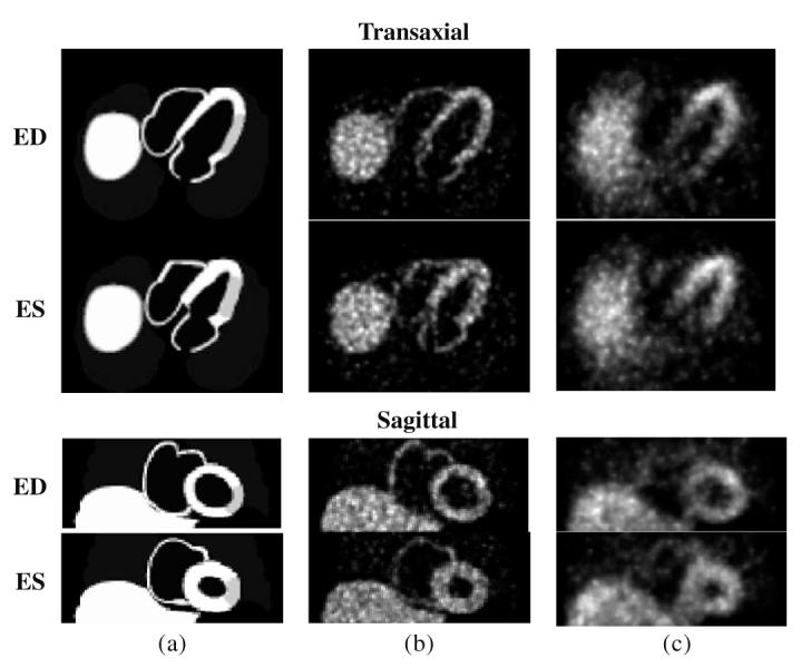
Example 2D slice images of the 4D NCAT phantom in transaxial and sagittal slice orientations at end-diastole (ED) and end-systole (ES) frames. (a) Noise-free phantom, (b) Set 1 images (without attenuation, scatter and detector response effects) and (c) Set 2 images (with attenuation, scatter and detector response effects).

Gated projection data of the phantom were computed using both a simple and a realistic physical model. We refer to the resulting images from the simple model as Set 1 and those from the realistic model as Set 2.

For the simple model, the effects of detector response, attenuation, scatter and randoms were not included in order to isolate the effects of statistical noise on the motion estimation. The data were computed using linear interpolation within the projection space for 60 angles over 180 degrees assuming parallel-ray geometry. The projection data were down-sampled to create 3 mm pixels and projection matrices that were 96 elements transaxially and 40 elements axially. Synthetic Poisson noise was added to the projection data after scaling the data to approximately 14 000 detected counts per frame within a 3 mm, mid-ventricular slice. This count level is representative of a clinical SPECT, gated myocardial perfusion study using Tc-99m sestamibi. An ensemble of 10 noisy datasets was generated in order to estimate the uncertainty in the measured results.

For the realistic model, projection data were computed using Monte Carlo simulation via the SIMIND program (Ljungberg and Strand 1989). The simulation modeled a SPECT acquisition including the effects of attenuation, scatter and detector response assuming 140 keV photon energy. The linear attenuation distribution that was input to the simulation was generated by the NCAT program, and a mid-ventricular, transaxial slice image of the attenuation distribution is shown in figure 2. This represented an average attenuation distribution across the eight frames. The simulation assumed a low energy, general purpose collimator, 15% energy resolution, 20% energy window, 25 cm radius of rotation and 64 angles over 180°. The sampling and count level were the same as in the simple case, and an ensemble of 10 noisy datasets was generated.

Figure 2.

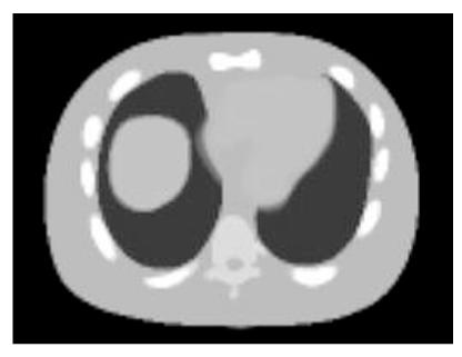
Transaxial slice of 4D NCAT attenuation distribution for Monte Carlo simulation.

The ensembles of noisy projection data for both the simple and realistic models were reconstructed by OSEM (Hudson and Larkin 1994). For the simple model (Set 1), the 60 projection angles were divided into 10 subsets; for the realistic model (Set 2), the 64 angles were divided into 8 subsets. The reconstructed image matrices were 96 × 96 transaxially with 40 axial slices. The reconstruction was stopped after five iterations and a post-reconstruction, 3D Butterworth filter was applied to each of the eight reconstructed frames. For the Set 1 images, the filter parameters were a cut-off frequency of 0.6 cm^-1 and a power of 5. These were the filter parameters that resulted in the most accurate motion estimation from our earlier work (Mair et al 2006) using the motion estimation method of Klein et al (1997). For the Set 2 images, the filter cut-off frequency was reduced to 0.4 cm^-1. The Set 2 images had a higher noise level relative to the Set 1 images—due to the same number of detected counts being spread over a wider detector area—and so the smoother filter cut-off frequency was preferable from a subjective image quality standpoint. Figures 1(b) and (c) show the Set 1 and Set 2 reconstructed images, respectively, for one noise realization including ED and ES frames at transaxial and sagittal slice planes.

2.4. Physical phantom study

The motion estimation methods were also tested on reconstructed images obtained from a dynamic, physical phantom¹ containing radioactivity in the myocardial chamber. In order to assess the accuracy of the estimated motion with these phantom images, the true motion of the myocardium was independently measured using radioactive point markers attached to the epicardial surface of the myocardium. The marker and myocardial data acquisitions (described below) were performed in such a way that ensured co-registration of the images without cross contamination effects.

The phantom contains two latex membranes that defined the ‘myocardium’ and ‘ventricle’ chambers, which are separately fillable. A computer-controlled, motorized pump moves water in and out of the ventricle chamber based on a programmed volume-time curve. The phantom also contains two ‘lungs’, consisting of Styrofoam beads and water, and a Teflon ‘spine’ to model patient attenuation characteristics. Figure 3 shows a photograph of the phantom.

Figure 3.

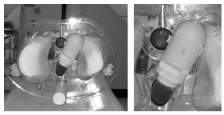
Photograph of beating heart phantom showing myocardial markers. The outer shell of the phantom has been removed.

Ten radioactive markers were constructed from latex tubing (1.6 mm I.D.) cut into approximately 4 mm segments. The ends of the tube segments were sealed with rubber cement. Using a syringe, the tube segments were injected with the Tc-99m solution at an activity of approximately 3 mCi per marker. The markers were attached with uniform spacing to the outer wall of the latex phantom myocardium using rubber cement. A photograph of the phantom with the attached markers is shown in figure 3.

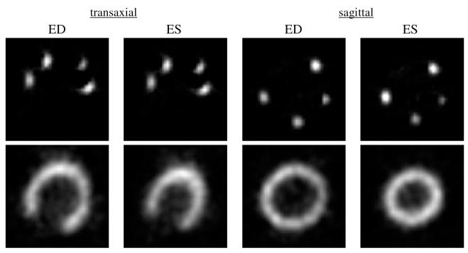
The phantom was filled with water, and gated SPECT data were acquired on a commercial SPECT system². The phantom operated at 60 beats min^-1 with 65 mL stroke volume and 50% ejection fraction. A long scan (3 h) was performed in order to assure low noise in the marker data. Acquisition parameters included the following: 120 projection angles over 360 degrees, 128 × 64 projection matrix (3.6 mm pixel size), 8 gated frames per heart cycle, low-energy, ultra-high resolution collimator and 15% energy window. The marker projection data were reconstructed by OSEM using 12 subsets, 50 iterations and without attenuation or scatter correction. No filtering was applied due the low noise level of the images. The reconstructed marker images are shown in the top row of figure 4 in transaxial and sagittal slice orientations at the ED and ES frames. For each marker, the 3D centroid of activity was computed over all eight gated frames using regions-of-interest that isolated each marker. The motion of the ten centroids over the eight frames provided an estimate of the true wall motion for pixels adjacent to the centroid locations.

Figure 4.

Reconstructed images of marker activity (top row) and myocardial activity (bottom row) for the physical, beating heart phantom.

The myocardial data acquisition followed the marker data acquisition after the marker activity was allowed to decay to a negligible level (after 68 h) and without moving the phantom between the two acquisitions. The phantom myocardium was injected with the Tc-99m solution through an access port. No radioactivity was placed outside of the myocardium. The goal was to obtain low noise data, from which simulated Poisson noise could be added at any desired count level. Therefore, the injected activity was 73 mCi and a series of SPECT acquisitions were performed totaling 8 h of scan time. For this study, the projection data were scaled, before adding simulated Poisson noise, to a count level of approximately 215 000 counts in a mid-ventricular, 3.6 mm thick transaxial slice (summed over all frames). This count level is in a range between clinical gated Tc-99m-sestamibi SPECT and F-18-FDG cardiac PET. The acquisition parameters were the same as for the marker data acquisition. The acquired data were reconstructed using OSEM with 20 subsets, 6 projection angles per subset and 10 iterations. The reconstructed images within each gated frame were filtered using a 3D Hann filter with a cut-off frequency equal to the Nyquist frequency. These reconstruction parameters were empirically chosen to achieve a balance of spatial resolution and noise control. The reconstructed images of myocardial activity are shown in the bottom row of figure 4 in transaxial and sagittal slice orientations at the ED and ES frames. These images were used as the test images for the motion estimation methods.

2.5. Motion error metrics

With the simulated phantom images, the estimated motion error was evaluated using a metric that we term the phantom-matching motion error (PME) and defined as

$$PME\left(\mathbf{m}\right)=\sum _{\mathbf{r}}\sum _n{({\stackrel{‒}{f}}_n\left(\mathbf{r}\right)-{\stackrel{‒}{f}}_{n+1}(\mathbf{r}+{\mathbf{m}}_n\left(\mathbf{r}\right)))}^2$$ (10)

where ${\stackrel{‒}{f}}_n\left(\mathbf{r}\right)$ is the true phantom intensity image at frame n, and m_n(r) is the estimated motion from frames n to n + 1. It is expected that the true motion should have a PME that is close to zero. For this study, the summation was confined to a region-of-interest that included the left myocardium and a small region (approximately one voxel wide) surrounding the left myocardium (figure 5). The mean PME and standard deviation across the ensemble of results were computed. For the Set 2 images, the PME is also reported for each of the eight frame intervals.

Figure 5.

One slice of the 4D region-of-interest (left) and the corresponding phantom image (right) used for the PME measurement.

With the physical phantom images, the estimated motion error was the Euclidean error between the marker motion (‘true’ motion) and the average motion of the eight closest voxels to each marker. This error was averaged over all ten markers. The error is reported for the frame 1-2 interval and averaged over all eight frame-to-frame intervals. The frame 1-2 interval with this phantom exhibits substantially greater average marker motion magnitude than all other intervals as evidenced by the true marker motion in table 1.

Table 1.

Average true marker motion magnitude (pixel units)

Frame interval	1-2	2-3	3-4	4-5	5-6	6-7	7-8	8-1
Average magnitude	0.94	0.28	0.22	0.46	0.31	0.19	0.21	0.17

2.6. Image reconstruction using estimated motion

We incorporated the estimate motion from the HS and SQ-HS methods into a 4D image reconstruction method and evaluated the resulting reconstructed image quality using the physical phantom data. The reconstruction method uses the estimated motion in the penalty term of a penalized maximum likelihood (PML) algorithm. The penalty term is identical to the optical flow term in equation (2) except that the motion vector field m is fixed, and an optimal f is computed using the R step reconstruction algorithm in Mair et al (2006). This reconstruction algorithm is a modification of the one-step-slate algorithm of Green (1990) that has improved convergence properties. The PML reconstructed images were compared with those obtained by OSEM and 3D post-reconstruction filtering with a Hann filter.

3. Results

3.1. Simulated phantom study

Figure 6 shows plots of PME as a function of β for the HS method applied to the Set 1 (left) and Set 2 (right) images. Both curves exhibit an optimal β but at different values of β. The lower value for the Set 2 case is due to the lower image intensities for this case, which affects the magnitude of the optical flow function and, therefore, the balance of the optical flow function and smoothness constraint. The standard deviation across the ensemble of measurements was less than 2.5% of the mean for all data points in figure 6.

Figure 6.

Motion estimation error as a function of the penalty parameter β for the HS method. Left: Set 1 images and right: Set 2 images.

Figure 7 shows ‘double-y’ plots of PME as a function of the SQ-HS iteration number for the noise-free phantom (left) and noisy reconstructed images (right). The values forβ that were used were close to the optimum for all cases (0.001 for Set 1, noise-free; 0.0001 for Set 2, noise-free; 0.01 for Set 1, noisy and 0.002 for Set 2, noisy). The reader is reminded that the first SQ-HS iteration is equivalent to the HS method. Both plots demonstrate a decrease in error with iteration and the clear improvement in motion estimation accuracy with the SQ-HS method relative to the HS method. The noise-free case attains a smaller error, which illustrates the substantial impact of image noise on the motion estimation. The standard deviation across the ensemble of measurements was less than 5% of the mean for all data points in figure 7.

Figure 7.

Motion estimation error as a function of the SQ-HS iteration number. Left: noise-free images and right: noisy images. In both plots, the left and right axes refer to Set 1 and Set 2 images, respectively.

Table 2 shows the PME error (Set 2 images) for the HS and SQ-HS methods on a frame-by-frame basis. Also shown are the average motion vector magnitudes within the region-of-interest for both methods and for the NCAT-defined motion. The PME results show that the SQ-HS method was more accurate (smaller average motion error) relative to the HS method for all but one of the eight frame intervals. The intervals in which the difference was largest—for example, intervals 1-2 and 2-3—tended to be the intervals of largest average motion magnitude, based on the NCAT-defined motion. The exception to this was the 6-7 interval. Comparing the estimated vector magnitudes between the two methods shows that SQ-HS resulted in a larger magnitude than HS at all intervals and closer to the NCAT-defined magnitudes. Both methods, however, were substantially smaller than the NCAT-defined magnitude.

Table 2.

Frame-by-frame results (Set 2 images)

		Frame interval
		1→2	2→3	3→4	4→5	5→6	6→7	7→8	8→1
PME	HS	16.2	13.5	8.9	8.7	10.9	14.1	8.2	13.1
	SQ-HS	13.4	11.9	8.9	8.4	10.2	13.7	8.0	12.7
Average magnitude	HS	0.36	0.37	0.26	0.25	0.29	0.40	0.24	0.31
	SQ-HS	0.55	0.56	0.40	0.36	0.43	0.53	0.34	0.44
	NCAT	1.41	0.99	0.62	0.61	0.92	1.47	0.57	0.69

Figures 8 and 9 show the quiver plots of the estimated motion vector fields (2D component of the 3D vectors) from the Set 1 and Set 2 images, respectively, superimposed on a mid-ventricular, sagittal slice of the noise-free phantom images. The results are for a mid-systole frame interval (frame 1 to 2). Both figures show the HS and SQ-HS results along with the NCAT program motion vectors. A magnified region of the myocardium is included for better visualization of the motion vectors. In these examples, the SQ-HS result is in closer agreement with the NCAT result and demonstrates the larger motion magnitude than the HS result. Both methods perform better with the Set 1 images in terms of the similarity in magnitude and direction with the NCAT result. This provides an illustration of the degrading effects of attenuation, scatter and detector response on the motion estimation accuracy in uncompensated images.

Figure 8.

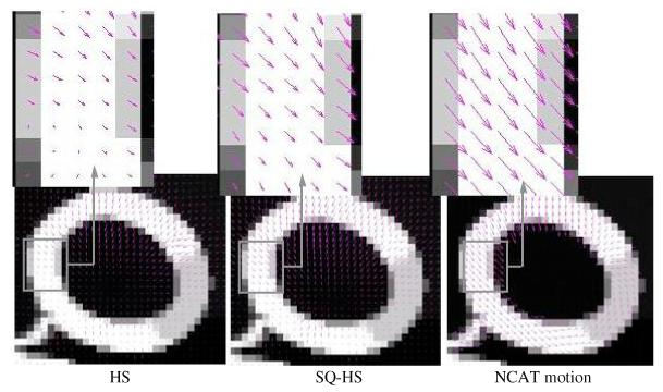
Estimated motion vector fields from the Set 1 images superimposed on noise-free phantom images. The results are for a mid-systole frame interval (frame 1 to 2).

Figure 9.

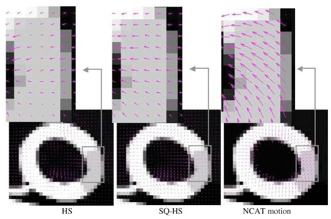
Estimated motion vector fields from the Set 2 images superimposed on noise-free images. The results are for a mid-systole frame interval (frame 1 to 2).

Figure 10 presents the convergence results, which are plots of the respective objective function versus iteration, for the HS and SQ-HS methods applied to a single noisy dataset of the Set 1 and Set 2 images. For HS, the objective function is the sum of the quadratic optical flow term and the smoothness constraint, which is equation (5) with fixed m̃(r) = 0. For SQ-HS, the objective function is the sum of the non-quadratic optical flow term and the smoothness constraint and is given by equation (1). For both HS and SQ-HS, the objective function is summed over all eight frame intervals. Each SQ-HS iteration includes the ‘inner’ iterative process described in section 2.2. The results in figure 10 demonstrate the monotonic convergence of both methods. It is interesting to note the degree to which the SQ-HS method achieves a smaller value of the non-quadratic objective function compared with the HS method. Evaluating equation (1) using the HS estimate at convergence for the Set 1 case from figure 10 resulted in value of 1596, which is greater than the SQ-HS value for Set 1 from figure 10 of 1439.

Figure 10.

Objective function value versus iteration for the HS (left) and SQ-HS (right) methods.

The computation time was determined for the HS and SQ-HS algorithms to estimate the motion vector fields for the 96 × 96 × 40 voxels across eight frames. The HS method required 90 iterations, and the cpu time on a modern workstation³ with a 3.6 GHz processor was 22 s. The SQ-HS method required 20 iterations, and the cpu time was 116 s.

3.2. Physical phantom study

Figure 11 shows plots of the Euclidean error as a function of β for the frame 1-2 interval and averaged over all frame intervals. For the frame 1-2 interval, the SQ-HS method resulted in a smaller minimum error (0.319 at β = 0.1) compared with HS (0.365 atβ = 0.05). Averaged over all frame intervals, the SQ-HS method demonstrated only a marginally reduced minimum error compared with HS. Given the average frame-to-frame motion magnitudes with this phantom (table 1), these results indicate that the improved performance of SQ-HS compared with HS becomes more pronounced with greater motion magnitude.

Figure 11.

Motion estimation error as a function of β for the physical phantom images. Left: frame 1-2 interval and right: averaged over all frame intervals.

Figure 12 shows the estimated motion vector fields (2D component of the estimated 3D vector) superimposed on a reconstructed coronal image for HS (left column) and SQ-HS (right column) for the frame 1-2 interval. For both methods, the optimal β for this interval was used (0.05 for HS and 0.1 for SQ-HS). The top row in this figure shows the magnified region in the neighborhood of one of the ten markers, and the marker motion (2D component) for the frame 1-2 interval is indicated by the black vector. The SQ-HS estimated motion is in closer agreement with the marker motion compared with the HS estimated motion, which is erroneously small in magnitude. The bottom row in this figure shows the magnified view of another region that demonstrates differences between the two methods in terms of the smoothness in the estimated motion. The HS result shows greater discontinuity in the estimated vector field. Improvement in this regard can be achieved by using a value of β larger than 0.05; however, this increases the overall error, as evidenced in figure 11(left), due to a reduced estimated motion magnitude.

Figure 12.

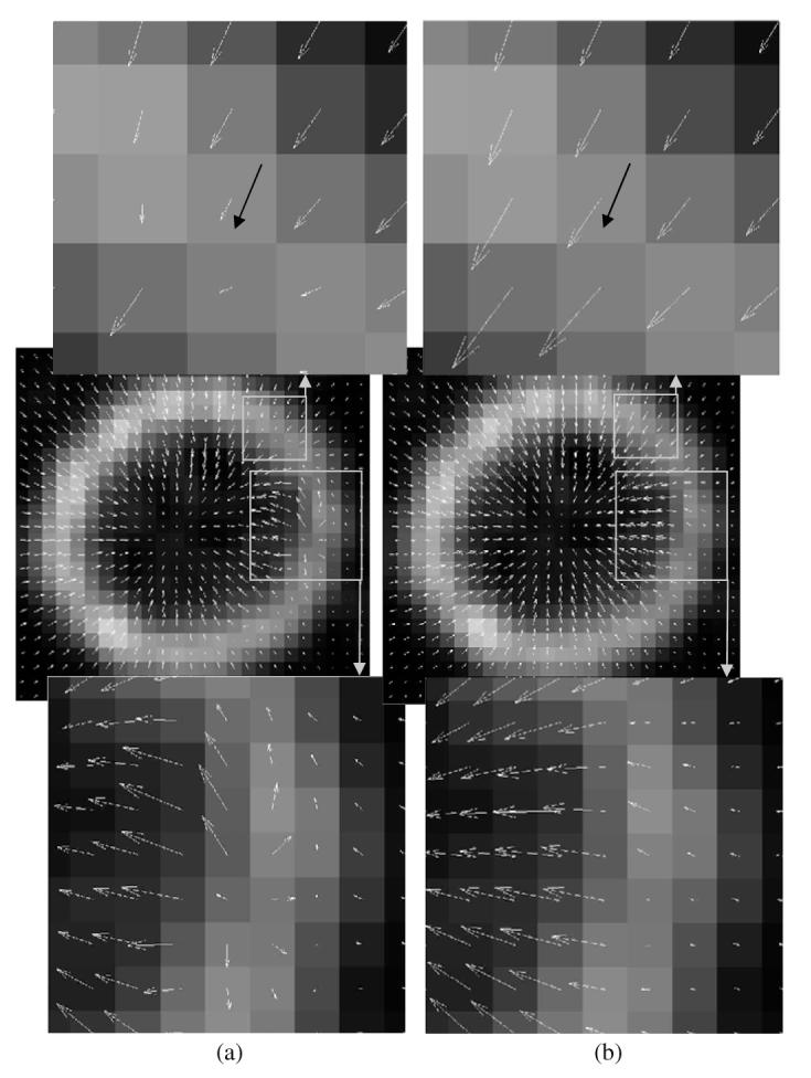
Estimated motion vector fields superimposed on a reconstructed image of the physical phantom data for the frame 1-2 interval. (a) HS method and (b) SQ-HS method.

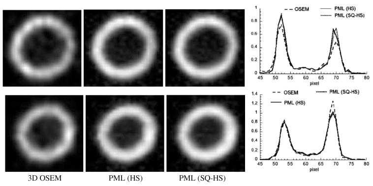
Figure 13 shows the results of the 4D motion-compensated reconstructed images. Both the HS and SQ-HS estimates were used with their optimal β for the frame 1-2 interval (0.05 for HS and 0.1 for SQ-HS). Also shown are the OSEM images with 3D post-reconstruction filtering. The cut-off frequency of the 3D filter (1.4 cycles cm^-1) was chosen empirically to produce a subjectively acceptable resolution/noise trade-off. The images and profiles in the figure show that the PML images, relative to the OSEM images, have a more uniform intensity throughout the wall region, which more accurately depicts the truly uniform radioactivity distribution within the wall region. This can be attributed to the ability of the PML method to control noise by correlating pixel intensities across frames along the estimated lines of motion. The difference between the PML methods using the HS and SQ-HS motion estimates is not substantial.

Figure 13.

3D OSEM versus PML using the HS and SQ-HS motion estimates. Top row: frame 1, bottom row: frame 2. Profiles were taken along the middle, horizontal pixel row.

4. Summary and discussion

This paper presents a new method for estimating the 3D, non-rigid motion between sequential frames in a time series of images. The method is a generalization of a standard optical flow motion estimation algorithm that formulates the problem in a successive quadratic approximation framework. In the evaluation with mathematical and physical phantom images, the method resulted in reduced estimated motion error relative to the standard optical flow algorithm. The improvement was generally greater within frame intervals with larger magnitude motion. This result may be related to the linearized OFC of the standard algorithm, which assumes that motion magnitude is relatively small. Convergence of the new method was evidenced with a monotonically decreasing objective function value with iteration. The computer processing time required to estimate the motion vector fields for a 96 × 96 × 40 voxel image over eight time frames was approximately 2 min on a modern workstation.

In addition to its use in assessing cardiac wall motion, the proposed method can be used within 4D motion-compensated reconstruction methods, which have been described in several earlier works. While clear improvement in motion estimation accuracy was observed with the proposed method, comparable image quality was observed when the motion estimates by the standard and proposed methods were incorporated into a 4D reconstruction of SPECT data. The lack of definitive improvement in this context may not necessarily generalize to other contexts in which spatial resolution and image noise degradation are less severe, such as in cardiac PET. Other applications for the proposed method include 4D reconstruction in cardiac CT angiography.

The question arises how to choose a reasonable value for the penalty parameter β in the realistic situation in which there is no knowledge of the true motion. In our initial implementation with clinical data, β has been chosen empirically based on the characteristics of the estimated motion vector fields. Vectors that are clearly too small in magnitude indicate that β is too large; the estimation is overly constrained. As β is allowed to decrease, the estimated motion vectors increase in magnitude yet adjacent pixels maintain a (subjectively) reasonable degree of continuity in direction and magnitude. As β decreases beyond this, the motion vectors at adjacent pixels become unrealistically dissimilar, and we know that the choice of β is too small. Perhaps the most critical issue to affect the choice of β is the count level in the images since this affects the magnitude of the optical flow term (a function of f) but not the smoothness constraint (not a function of f). Within a given clinical procedure, with a fixed injected dose and scan time, the expected variation in count level may be small enough that a single value of β is satisfactory for all cases (although factors such as uptake percentage and attenuation would still introduce count level variation across cases). If not, it may be possible to normalize the images before motion estimation to achieve satisfactory performance across cases using a single value for β. Future work will investigate the robustness of these methods to the choice of β within a given class of patient images.

References

- Alvarez L, Weickert J, Sanchez J. Reliable estimation of dense optical flow fields with large displacements. Int. J. Comp. Vis. 2000;39:41–56. [Google Scholar]
- Black MJ, Anandan P. The robust estimation of multiple motions: parametric and piecewise-smooth flow fields. Comput. Vis. Image Understand. 1996;63:75–104. [Google Scholar]
- Brankov JG, Yang Y, Wernick MN. Spatiotemporal processing of gated cardiac SPECT images using deformable mesh modeling. Med. Phys. 2005;32:2839–49. doi: 10.1118/1.2013027. [DOI] [PubMed] [Google Scholar]
- Cunningham GS, Hanson KM, Battle XL. Three-dimensional reconstructions from low-count SPECT data using deformable models. Opt. Exp. 1998;2:227–36. doi: 10.1364/oe.2.000227. [DOI] [PubMed] [Google Scholar]
- Feng B, Bruyant PP, Pretorius PH, Beach RD, Gifford HC, Dey J, Gennert MA, King MA. Estimation of the rigid body motion from three dimensional images using a generalized center-of-mass points approach. IEEE Trans. Nucl. Sci. 2006;53:2712–8. doi: 10.1109/TNS.2006.882747. [DOI] [PMC free article] [PubMed] [Google Scholar]
- Gravier E, Yang Y, King MA, Jin M. Fully 4D motion compensated reconstruction of cardiac SPECT images. Phys. Med. Biol. 2006;51:4603–19. doi: 10.1088/0031-9155/51/18/010. [DOI] [PubMed] [Google Scholar]
- Green P. Bayesian reconstructions from emission tomography using a modified EM algorithm. IEEE Trans. Med. Imaging. 1990;9:84–93. doi: 10.1109/42.52985. [DOI] [PubMed] [Google Scholar]
- Horn BKP, Schunck BG. Determining optical flow. Artif. Intell. 1981;17:185–203. [Google Scholar]
- Hudson H, Larkin R. Accelerated image reconstruction using ordered subsets of projection data. IEEE Trans. Med. Imaging. 1994;13:601–9. doi: 10.1109/42.363108. [DOI] [PubMed] [Google Scholar]
- Klein GJ, Huesman RH. Elastic material model mismatch effects in deformable motion estimation. IEEE Trans. Nucl. Sci. 2000;47:1000–5. [Google Scholar]
- Klein GJ, Reutter BW, Huesman RH. Non-rigid summing of gated PET via optical flow. IEEE Trans. Nucl. Sci. 1997;40:1509–12. [Google Scholar]
- Laading JK, McCulloch C, Johnson VE, Gilland DR, Jaszczak RJ. A hierarchical feature based deformation model applied to 4D cardiac SPECT data Information Processing in Medical Imaging: Lecture Notes in Computer Science. Springer; Berlin: 1999. pp. 266–79. [Google Scholar]
- Lalush DS, Tsui BMW. Block iterative techniques for fast 4D reconstruction using a priori motion models in gated cardiacSPECT. Phys. Med. Biol. 1998;43:875–86. doi: 10.1088/0031-9155/43/4/015. [DOI] [PubMed] [Google Scholar]
- Ljungberg M, Strand S-E. A Monte Carlo program simulating scintillation camera imaging. Comput. Methods Programs Biomed. 1989;29:257–72. doi: 10.1016/0169-2607(89)90111-9. [DOI] [PubMed] [Google Scholar]
- Maintz JBA, Viergever MA. A survey of medical image registration. Med. Image Anal. 1998;2:1–36. doi: 10.1016/s1361-8415(01)80026-8. [DOI] [PubMed] [Google Scholar]
- Mair BA, Gilland DR, Sun J. Estimation of images and non-rigid deformations in gated emission CT. IEEE Trans. Med. Imaging. 2006;25:1130–44. doi: 10.1109/tmi.2006.879323. [DOI] [PubMed] [Google Scholar]
- Makela T, et al. A review of cardiac image registration methods. IEEE Trans. Med. Imaging. 2002;21:1011–21. doi: 10.1109/TMI.2002.804441. [DOI] [PubMed] [Google Scholar]
- Rueckert D, Sonoda LI, Hayes C, Hill DLG, Leach MO, Hawkes DJ. Nonrigid registration using free-form deformations: application to breast MR images. IEEE Trans. Med. Imaging. 1999;18:712–21. doi: 10.1109/42.796284. [DOI] [PubMed] [Google Scholar]
- Segars WP, Lalush DS, Tsui BMW. A realistic spline-based dynamic heart phantom. IEEE Trans. Nucl. Sci. 1999;46:503–6. [Google Scholar]
- Song SM, Leahy RM. Computation of 3-D velocity fields from 3-D cine CT images of a human heart. IEEE Trans. Med. Imaging. 1991;10:295–306. doi: 10.1109/42.97579. [DOI] [PubMed] [Google Scholar]
- Turkington TG, DeGrado TR, Hanson MW, Coleman RE. Alignment of dynamic cardiac PET images for correction of motion. IEEE Trans. Nucl. Sci. 1997;44:235–42. [Google Scholar]