Backward Bifurcations and Multiple Equilibria in Epidemic Models with Structured Immunity

Abstract

Many disease pathogens stimulate immunity in their hosts, which then wanes over time. To better understand the impact of this immunity on epidemiological dynamics, we propose an epidemic model structured according to immunity level that can be applied in many different settings. Under biologically realistic hypotheses, we find that immunity alone never creates a backward bifurcation of the disease-free steady state. This does not rule out the possibility of multiple stable equilibria, but we provide two sufficient conditions for the uniqueness of the endemic equilibrium, and show that these conditions ensure uniqueness in several common special cases. Our results indicate that the within-host dynamics of immunity can, in principle, have important consequences for population-level dynamics, but also suggest that this would require strong non-monotone effects in the immune response to infection. Neutralizing antibody titer data for measles is used to demonstrate the biological application of our theory.

1 Introduction

One of the major undertakings of epidemiological modeling is to describe how changes in biological processes will effect the characteristics of the infection dynamics at a population level. A major early result of this work, derived from elementary models, is the “R₀ dogma” (Anderson and May, 1991; May et al., 2001). R₀, the basic reproductive ratio, represents the expected number of new infections caused by each case of infection at the start of an epidemic in a certain baseline population (most often, a naive population) (Macdonald, 1952). If R₀ > 1, the number of infections after an initial introduction grows, creating an epidemic. If R₀ < 1, small initial introductions are not sufficiently transmissible to cause an epidemic; a new epidemic can not be started and an endemic disease will fade out. Thus, many control policies like vaccination have focused on reaching coverage levels sufficient to reduce R₀ below 1.

Over the last fifteen years, one of the important issues in epidemiological modeling has been understanding when and how the R₀ dogma can fail. In particular, some epidemic models can be bistable: R₀ < 1 is a sufficient condition for avoiding an epidemic caused by the introduction of a small number of initial cases, but R₀ < 1 is not a sufficient condition for eradication of the disease once it is endemic. One common way to identify bistable epidemic models is to look for backward bifurcations. In SIR models, the transcritical bifurcation at R₀ = 1 typically has two locally stable branches: a disease-free branch that is locally stable for R₀ < 1, and an endemic-disease branch that is stable for R₀ > 1. As the basic reproductive ratio is varied through the bifurcation, the asymptotic dynamics of the system under small perturbations change continuously between these two branches. This is called a forward bifurcation. A model has a backward bifurcation if only one of the three biologically feasible branches of the transcritical bifurcation in the neighborhood of R₀ = 1 is locally stable. Because the remaining two biologically feasible branches (corresponding to non-negative population states) are locally unstable, variations in the basic reproductive ratio lead to discontinuous changes in the asymptotic dynamics of the system. A small increase in the transmission rate causes a large increase in the number of disease cases. A subsequent small decrease in the transmission rate does not lead to the sudden disappearance of an endemic disease.

The R₀ dogma can potentially lead to serious miscalculations when a model exhibits a backward bifurcation or other forms of bistability, so it is important to understand the circumstances that can create a backward bifurcation. For instance, behavior changes can be important. Backward bifurcations can occur when the investment of individuals in protective behaviors is inversely correlated with disease prevalence (Reluga and Medlock, 2007). Another mechanism that may change the equilibrium structure of epidemic models is acquired immunity, but this has received limited attention. Several papers have shown that models with acquired immunity can have backward bifurcations (Arino et al., 2003; Feng et al., 2000; Kribs-Zaleta and Velasco-Hernandez, 2000; Gomes et al., 2005). However, the bifurcations in these papers only occur for parameter ranges where infection “accelerates” the waning of immunity, a situation that disagrees with our understanding of tuberculosis (Lipsitch and Murray, 2003) and other vaccine-preventable diseases. In a previous paper (Reluga and Medlock, 2007), we conjecture that under a biologically reasonable hypothesis, immunity will not introduce backward bifurcations into a model. Specifically, this hypothesis assumes that immunity always increases under repeated exposure, in the sense that it provides greater protection and faster recovery, and that immunity wanes monotonely.

This paper analyzes a model of acquired immunity in the absence of demographic effects, behavioral changes, and artificial control measures like vaccination. We prove that for a general class of models with immunity satisfying our immunological hypothesis, there are no backward bifurcations. We show by counter-example that this does not exclude the possibility of multiple steady-state solutions. We go on to provide a sufficient condition for uniqueness of the endemic equilibrium, excluding the possibility of multiple steady-state solutions, and indicating when the traditional R₀ dogma can be safely applied. As an application, we parameterize our model using measles antibody data and show that it does not have a backward bifurcation in that case. This parameterization does not satisfy our conditions for ruling out multiple endemic equilibria, but we numerically observe only one endemic equilibrium.

2 Modeling

To help us understand the possible impacts of immunity on the bifurcation structure of an endemic disease, we will use a simple but general model of acquired immunity. In many models of infectious disease transmission, immunity is treated in a binary way: immunity is either present or absent. In the large, this seems like a reasonable assumption since individuals exposed to infection either become infected or do not become infected, and among individuals who become infected the course of infection is often very similar. However, a deeper inspection of the immunology and epidemiology shows the situation to be significantly more complex. In our current understanding of immunology, it is clear that an individual’s immunity state depends on the types and numbers of memory B and T cells and is a consequence of stochastic processes so sensitive to historical conditions that different individuals can easily create dramatically different immune responses to the same pathogen (Kuby, 1994). We also know that immune state can have important consequences for the course of infection (Kuby, 1994). A recent study has shown that while antibodies to viral infections may not have significant decay over a person’s lifetime, B-cell memory may still decay (Amanna et al., 2007). T cell memory may also be susceptible to decay over time (Homann et al., 2001). In light of these points, perhaps it is more natural when modeling the transmission of infectious diseases to allow individuals to occupy one of many different immunity states and to let the course of infection depend on the specific immunity state.

Consider a system of ordinary differential equations with n immunity states. We avoid demographic complications by assuming that there is no birth or death; the total size of the population remains constant at N > 0. Let S_j be the number of susceptible individuals in immunity state j and I_j be the number of infected individuals who had immunity state j when they were infected. The probability that an individual in immunity state j becomes infected relative to an individual in immunity state 1 is σ_j, with 0 ≤ σ_j ≤ 1 and σ₁ = 1. Individuals with immunity j remain infected on average for time 1/γ_j, where γ_j > 0. When an individual recovers, the individual’s immunity state changes from state i to state j with probability f_ij, with 0 ≤ f_ij ≤ 1 and Σ_j f_ij = 1. In addition, immunity in susceptibles spontaneously wanes from state i to state j at rate g_ij ≥ 0. The model is given by the differential equations

$$\frac{{\mathrm{d}S}_j}{\mathrm{d}t}=\sum _{i=1}^n{g}_{\mathit{ij}}{S}_i-S_j\sum _{i=1}^n{g}_{\mathit{ji}}-{\beta I}_{\mathrm{Total}}{\sigma }_j{S}_j+\sum _{i=1}^n{\gamma }_i{I}_i{f}_{\mathit{ij}},$$ (2.1a)

$$\frac{{\mathrm{d}I}_j}{\mathrm{d}t}={\beta I}_{\mathrm{Total}}{\sigma }_j{S}_j-{\gamma }_j{I}_j,$$ (2.1b)

for j = 1, … , n, where

$$I_{\mathrm{Total}}=\sum _{j=1}^n{I}_j,\mathrm{and}N=I_{\mathrm{Total}}+\sum _{j=1}^n{S}_j.$$ (2.1c)

The use of I_Total to parameterize the force of infection corresponds to assuming the infectivity of individuals is independent of the immunity level. Without loss of generality we take N = 1 and γ₁ = 1, which amount to rescaling S_j and I_j by N and rescaling β, γ_j, g_ij, and t by γ₁. Since the population size is fixed, System (2.1) may be interpreted as either a standard-incidence or a bilinear-incidence model.

System (2.1) is a general model in the sense that it allows for arbitrary transitions between immunity states upon recovery and arbitrary degrees of protection for each immunity state. It also allows the immunity state to transition arbitrarily as it wanes. When thinking about changes in immunity within individuals, however, we expect the changes to be significantly simpler than this. Repeated exposure should increase immunity by both decreasing infection risk and speeding recovery. We also expect immunity to wane sequentially, such that each individual passes through all intermediate states as they lose immunity. We mathematically formalize these expectations, in terms of System (2.1), as the Immunity Dynamics Hypothesis (IDH).

Immunity Dynamics Hypothesis (IDH)

The structured dynamics of naturally acquired immunity in a population with an adaptive immune system are described by System (2.1) with the additional conditions that for every pair of integers i, j ∈ {1, 2, … n}:

• Risk of infection decreases with immunity state: σ_i ≤ σ_j if i > j,

• Recovery rate increases with immunity state: γ_i ≥ γ_j if i > j,

• Infection does not decrease immunity state: f_ij = 0 if i > j,

• Immune waning decreases immunity state sequentially: $\{\begin{array}{cc}{g}_{\mathit{ij}}>0& \mathit{if}i=j+1,\\ g_{\mathit{ij}}=0& \mathit{if}i\ne j+1.\end{array}$

There are certainly biological circumstances where the IDH does not hold, but it is a reasonable and general first cut.

Under the IDH, System (2.1) reduces to

$$\frac{\mathrm{d}{S}_j}{\mathrm{d}t}=g_{j+1}{S}_{j+1}-g_j{S}_j-\beta I_{\mathrm{Total}}{\sigma }_j{S}_j+\sum _{i=1}^j{\gamma }_i{I}_i{f}_{\mathit{ij}},$$ (2.2a)

$$\frac{\mathrm{d}{I}_j}{\mathrm{d}t}=\beta I_{\mathrm{Total}}{\sigma }_j{S}_j-{\gamma }_j{I}_j,$$ (2.2b)

$$I_{\mathrm{Total}}=\sum _{j=1}^n{I}_j,$$ (2.2c)

for j = 1, … , n, where, for convenience, we have defined g_j = g_j,j−1 with g₁ = g_n+1 = 0. The matrix F = [f_ij] is the immunization kernel. It describes the probability that an individual will transition from pre-infection immunity state i to post-infection immunity state j. The immunization kernel summarizes all the immune response dynamics of the model, and its structure can have important consequences for the model’s equilibrium structure. As we will see, System (2.2) has a relatively restricted range of equilibrium bifurcations.

3 Results

For all of the subsequent analysis, we will study the properties of the stationary solutions of System (2.2) under the IDH. We first derive an equation for I_Total at a stationary solution. Using this equation, we locate the epidemic bifurcation, show that System (2.2) does not have a backward bifurcation, and establish conditions that preclude multiple endemic equilibria.

At a stationary solution, the number of individuals in each state is constant over time, so the state variables S_j and I_j solve the polynomial equations

$$0=g_{j+1}{S}_{j+1}-g_j{S}_j-\beta I_{\mathrm{Total}}{\sigma }_j{S}_j+\sum _{i=1}^j{\gamma }_i{I}_i{f}_{\mathit{ij}},$$ (3.1a)

$$0=\beta I_{\mathrm{Total}}{\sigma }_j{S}_j-{\gamma }_j{I}_j$$ (3.1b)

$$1=I_{\mathrm{Total}}+\sum _{j=1}^n{S}_j.$$ (3.1c)

If I_Total were a constant, System (3.1) would be linear in the state variables and the stationary solutions could be calculated directly by elimination. We will take advantage of this by reducing the nonlinear part of the calculation to a scalar root-finding problem for I_Total and expressing the variables S_j and I_j in terms of I_Total.

First, let us consider Eq. (3.1b), which is equivalent to

$$I_j-\beta I_{\mathrm{Total}}\frac{{\sigma }_j}{{\gamma }_j}{S}_j=0.$$ (3.2)

Summing over all j, we find

$$I_{\mathrm{Total}}[1-\beta U]=0,\mathrm{where}U=\sum _{j=1}^n\frac{{\sigma }_j}{{\gamma }_j}{S}_j.$$ (3.3)

U can be interpreted as the “average” susceptibility of the population, and will be the focus of much of our analysis.

We will now show that the steady-state conditions can be manipulated to express U as a function of I_Total. Using Eq. (3.1b) to eliminate I_j, Eq. (3.1a) becomes

$$0=g_{j+1}{S}_{j+1}-g_j{S}_j-\beta I_{\mathrm{Total}}{\sigma }_j{S}_j+\sum _{i=1}^j\beta I_{\mathrm{Total}}{\sigma }_i{S}_i{f}_{\mathit{ij}}$$ (3.4)

or

$$g_{j+1}{S}_{j+1}=g_j{S}_j+\beta I_{\mathrm{Total}}{\sigma }_j{S}_j-\beta I_{\mathrm{Total}}\sum _{i=1}^j{f}_{\mathit{ij}}{\sigma }_i{S}_i.$$ (3.5)

Given I_Total, Eq. (3.5) represents a triangular homogeneous linear system for the S_j ’s. The solutions to this system lie in the one-dimensional subspace spanned by a vector x with components x_j given by

$$x_1=1,g_{j+1}{x}_{j+1}=g_j{x}_j+\beta I_{\mathrm{Total}}[{\sigma }_j{x}_j-\sum _{i=1}^j{f}_{\mathit{ij}}{\sigma }_i{x}_i],$$ (3.6)

Using recursive substitution to remove the g_jx_j terms,

$$x_1=1,x_{k+1}=\frac{\beta I_{\mathrm{Total}}}{g_{k+1}}\sum _{j=1}^k[{\sigma }_j{x}_j-\sum _{i=1}^j{f}_{\mathit{ij}}{\sigma }_i{x}_i].$$ (3.7)

Since the S_j’s solve Eq. (3.5), there must be some C such that C_xj = S_j for j = 1 … n. In addition, the S_j’s satisfy Eq. (3.1c), so by substituting and isolating, we show that

$$C=\frac{1-I_{\mathrm{Total}}}{{\sum }_{j=1}^n{x}_j}.$$ (3.8)

Thus, given I_Total, we can calculate the x_j’s as implicit functions of I_Total using Eq. (3.7), and we apply them to find

$$S_j=\frac{\left(1-I_{\mathrm{Total}}\right)x_j}{{\sum }_{k=1}^n{x}_k},$$ (3.9a)

$$I_j=\beta I_{\mathrm{Total}}\frac{{\sigma }_j}{{\gamma }_j}\frac{\left(1-I_{\mathrm{Total}}\right)x_j}{{\sum }_{k=1}^n{x}_k}.$$ (3.9b)

Substituting into Eq. (3.3), the stationary solution values of I_Total must solve the scalar equation

$$0=I_{\mathrm{Total}}[1-\beta U\left(I_{\mathrm{Total}}\right)],$$ (3.10)

where

$$U\left(I_{\mathrm{Total}}\right)=\sum _{j=1}^n\frac{{\sigma }_j}{{\gamma }_j}\frac{\left(1-I_{\mathrm{Total}}\right)x_j}{{\sum }_{k=1}^n{x}_k}$$ (3.11)

and

$$x_1=1,x_{k+1}=\frac{\beta I_{\mathrm{Total}}}{g_{k+1}}\sum _{i=1}^k\left[{\sigma }_i{x}_i(1-\sum _{j=i}^k{f}_{\mathit{ij}})\right].$$ (3.12)

This last equation for the x_j’s is just a rearrangement of the summation terms in Eq. (3.7).

The disease-free stationary solution to (2.2) is now easily calculated. One root of Eq. (3.10) is I_Total = 0. Using the condition g₀ = 0, we find that I_Total = 0 implies I_j = 0 for all j, S₁ = 1, and S_j = 0 for all j > 1. Thus, if infection is absent, so is immunity. Near the disease-free solution, the basic reproductive ratio is the transmission rate times the period of infection, or

$$R_0=\frac{\beta }{{\gamma }_1}=\beta ,$$ (3.13)

since γ₁ = 1. All stationary solutions other than the disease-free solution must correspond to roots of the equation 0 = 1 − βU (I_Total).

We can now see that the bifurcation structure of the stationary solutions in our model can be understood completely by studying U(I_Total). Since the waning rates are strictly positive, the x_j’s are uniquely determined for all I_Total and U (I_Total) is a well-defined function. The x_j’s are polynomial functions of I_Total and $0<{\sum }_{k=1}^n{x}_k<\infty$, so it follows from Eq. (3.11) that U(I_Total) is a smooth function of I_Total. On inspecting Eq. (3.11), we see that U(1) = 0. We can also show U(0) = 1. From the recurrence given in Eq. (3.12), if I_Total = 0 then x_j = 0 for all j > 1. Since σ₁ = γ₁ = x₁ = 1,

$$U\left(0\right)=\frac{\frac{{\sigma }_1}{{\gamma }_1}{x}_1+0+\cdots +0}{1+0+\cdots +0}(1-0)=1.$$ (3.14)

If R₀ = β = 1,

$$1-\beta U\left(0\right)=0.$$ (3.15)

So I_Total = 0 is a double root of Eq. (3.10) when β = 1. It follows that the epidemic bifurcation occurs at R₀ = 1, as expected.

3.1 Backward Bifurcations

U(I_Total) is continuous between I_Total = 0 and I_Total = 1, so the number of solutions to

$$\beta U\left(I_{\mathrm{Total}}\right)=1$$ (3.16)

in the interval [0, 1] is less than or equal to twice the number of local maxima (including possible maxima at the boundaries) of U(I_Total). If U(I_Total) is monotone decreasing, there will exist a unique solution for β > 1. By differentiating equilibrium condition (3.16) in the neighborhood of I_Total = 0, we can show that U is sufficiently monotone to preclude backward bifurcations.

Theorem 1

For System (2.2) under the IDH, the epidemic bifurcation at R₀ = 1 is never a backward bifurcation.

Proof

The direction of the bifurcation is given by the sign of $\frac{\mathrm{d}{I}_{\mathrm{Total}}}{\mathrm{d}\beta }$ when I_Total = 0. Thus, we will make a perturbation argument around the disease-free stationary solution. To determine the nature of the bifurcation, we differentiate equilibrium condition (3.16) with respect to β and find

$$U\left(I_{\mathrm{Total}}\right)+\beta \frac{\partial U}{\partial I_{\mathrm{Total}}}\frac{\mathrm{d}{I}_{\mathrm{Total}}}{\mathrm{d}\beta }+\beta \frac{\partial U}{\partial \beta }=0,$$ (3.17)

or

$$[-\frac{U\left(I_{\mathrm{Total}}\right)}{\beta }-\frac{\partial U}{\partial \beta }]{\left(\frac{\partial U}{\partial I_{\mathrm{Total}}}\right)}^{-1}=\frac{\mathrm{d}{I}_{\mathrm{Total}}}{\mathrm{d}\beta }.$$ (3.18)

When I_Total = 0, recurrence (3.12) implies

$$x_j=\{\begin{array}{cc}1& \mathrm{if}j=1,\\ 0& \mathrm{otherwise}.\end{array}$$ (3.19)

For small I_Total, the Maclaurin series approximation of recurrence relation (3.12) gives

$$x_j\approx \{\begin{array}{ll}1& \mathrm{for}j=1,\\ \frac{{\sigma }_1\beta I_{\mathrm{Total}}}{g_j}\left(1-{\sum }_{k=1}^{j-1}{f}_{1k}\right)& \mathrm{for}j=2,\cdots ,n-1.\end{array}$$ (3.20)

Using these Maclaurin series, the partial derivative of U with respect to I_Total is

$$\frac{\partial U}{\partial I_{\mathrm{Total}}}(I_{\mathrm{Total}}=0)=-{\sigma }_1-\sum _{j=2}^n\frac{{\sigma }_1\beta }{g_j}\left(\frac{{\sigma }_1}{{\gamma }_1}-\frac{{\sigma }_j}{{\gamma }_j}\right)\left(1-\sum _{k=1}^{j-1}{f}_{1,k}\right),$$ (3.21)

which is negative and decreasing in β because σ_j/γ_j ≤ σ₁/γ₁ for all j by the IDH. Also, since U(0) = 1, independent of β,

$$\frac{\partial U}{\partial \beta }=0.$$ (3.22)

It follows immediately from Eq. (3.18) that

$$\frac{\mathrm{d}{I}_{\mathrm{Total}}}{\mathrm{d}\beta }>0,$$ (3.23)

implying that the epidemic bifurcation is always a forward bifurcation, never a back-ward bifurcation.

Further, U(I_Total) ≤ 1 for all I_Total ≥ 0 since the IDH implies $\frac{{\sigma }_j}{{\gamma }_j}\le 1$ for all j. Thus, the disease-free stationary solution is the unique stationary solution for β < 1. These results might also be a special case of the general results presented recently by Boldin (2006), although we have not yet verified this.

3.2 Uniqueness

Having ruled out backward bifurcations for System (2.2) under the IDH, it is natural to ask if the IDH also implies a unique endemic stationary solution for β > 1. The answer is no. Even under the IDH, Eq. (3.16) can have multiple solutions.

Consider the following special case of our general model. Suppose there are 5 immunity states (n = 5), with the second, third, fourth, and fifth states respectively 5%, 30%, 60%, and 100% less susceptible than the first state. The waning and recovery rates are independent of state, i.e. g_j = g and γ_j = γ. Finally, on recovery, all state 1 individuals go to state 5, all state 2 individuals go to state 3, and all state 3 and state 4 individuals remain in their current states. State 5 individuals never become infected since their immunity is perfect (σ₅ = 0). The equations are

$$\frac{\mathrm{d}{S}_1}{\mathrm{d}t}=g{S}_2-\beta I_{\mathrm{Total}}{S}_1,$$ (3.24a)

$$\frac{\mathrm{d}{I}_1}{\mathrm{d}t}=\beta I_{\mathrm{Total}}{S}_1-I_1,$$ (3.24b)

$$\frac{\mathrm{d}{S}_2}{\mathrm{d}t}=g{S}_3-\frac{19}{20}\beta I_{\mathrm{Total}}{S}_2-g{S}_2,$$ (3.24c)

$$\frac{\mathrm{d}{I}_2}{\mathrm{d}t}=\frac{19}{20}\beta I_{\mathrm{Total}}{S}_2-I_2,$$ (3.24d)

$$\frac{\mathrm{d}{S}_3}{\mathrm{d}t}=g{S}_4-\frac{7}{10}\beta I_{\mathrm{Total}}{S}_3-g{S}_3+I_2+I_3,$$ (3.24e)

$$\frac{\mathrm{d}{I}_3}{\mathrm{d}t}=\frac{7}{10}\beta I_{\mathrm{Total}}{S}_3-I_3,$$ (3.24f)

$$\frac{\mathrm{d}{S}_4}{\mathrm{d}t}=g{S}_5-\frac{2}{5}\beta I_{\mathrm{Total}}{S}_4-g{S}_4+I_4,$$ (3.24g)

$$\frac{\mathrm{d}{I}_4}{\mathrm{d}t}=\frac{2}{5}\beta I_{\mathrm{Total}}{S}_4-I_4,$$ (3.24h)

$$\frac{\mathrm{d}{S}_5}{\mathrm{d}t}=-g{S}_5+I_1,$$ (3.24i)

The flow of immunity for System (3.24) is summarized in Figure 1.

Figure 1.

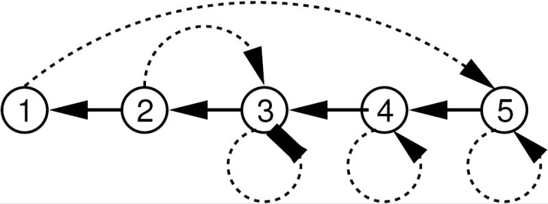
A directed graph of the flow of immunity in the counter example described by Eq. (3.24). Dotted arrows represent immunity gained following infection. Solid arrows represent waning immunity. The highest level of immunity can only be gained by individuals who become infected while in the first state.

Infection never decreases resistance, and the other assumptions of the IDH are met. There is no backward bifurcation at the R₀ threshold (i.e. varying β), but for sufficiently small g, there is an interval of β that gives multiple stationary solutions with positive prevalence (see Figure 2). Roughly speaking, these parameter values create multiple equilibria because high prevalence keeps most individuals in the intermediate immune states 2–4, while low prevalence leads to more of the population being in states 1 and 5, a higher level of population immunity.

Figure 2.

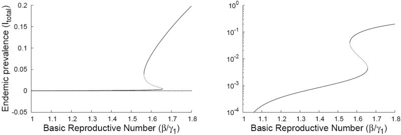
Plots of the disease incidence for stationary solutions to Eq. (3.24) as functions of the basic reproductive number β/γ₁. Our counter-example exhibits a forward bifurcation at β = 1 along with fold bifurcations at β = 1.56 and β = 1.65 when g = 1/300. For clarity, we have plotted the bifurcation structure on both arithmetic and semi-log axes.

We are left to determine which extra conditions are needed to ensure uniqueness of the solution to Eq. (3.16) for β > 1. One very useful idea is the concept of a stochastic ordering of the susceptible population states. A probability density p(x; u) over a subset of the real numbers is said to be stochastically decreasing with respect to the scalar parameter u if

$$\frac{\mathrm{d}}{\mathrm{d}u}{\mathit{\int }}_{-\infty }^{x}p(y;u)\mathrm{d}y\le 0\mathrm{for}\mathrm{all}x\text{.}$$ (3.25)

As the parameter u increases, the cumulative distribution of p(x; u) shifts right-ward. The susceptible states as functions of the total proportion infected I_Total are stochastically decreasing if

$$\frac{\mathrm{d}}{\mathrm{d}{I}_{\mathrm{Total}}}\sum _{j=1}^k{S}_j\left(I_{\mathrm{Total}}\right)\le 0\mathrm{for}\mathrm{all}k=1,\cdots ,n.$$ (3.26)

Theorem 2

For System (2.2) under the IDH, there is a unique endemic state for β > 1 if S_j(I_Total) is stochastically decreasing in I_Total.

Proof

Rearranging the summation in Eq. (3.3) gives

$$\begin{array}{ll}U& =\sum _{j=1}^n\frac{{\sigma }_j}{{\gamma }_j}{S}_j\\ & =\sum _{j=1}^{n-1}\left(\frac{{\sigma }_j}{{\gamma }_j}-\frac{{\sigma }_{j+1}}{{\gamma }_{j+1}}\right)\sum _{i=1}^j{S}_i+\frac{{\sigma }_n}{{\gamma }_n}\sum _{j=1}^n{S}_j\\ & =\sum _{j=1}^{n-1}\left(\frac{{\sigma }_j}{{\gamma }_j}-\frac{{\sigma }_{j+1}}{{\gamma }_{j+1}}\right)\sum _{i=1}^j{S}_i+\frac{{\sigma }_n}{{\gamma }_n}(1-I_{\mathrm{Total}}).\end{array}$$ (3.27)

Taking the derivative gives

$$\begin{array}{ll}\frac{\mathrm{d}U}{\mathrm{d}{I}_{\mathrm{Total}}}& =-\frac{{\sigma }_n}{{\gamma }_n}+\sum _{j=1}^{n-1}\left(\frac{{\sigma }_j}{{\gamma }_j}-\frac{{\sigma }_{j+1}}{{\gamma }_{j+1}}\right)\frac{\mathrm{d}}{\mathrm{d}{I}_{\mathrm{Total}}}\sum _{i=1}^j{S}_i\\ & \le \sum _{j=1}^{n-1}\left(\frac{{\sigma }_j}{{\gamma }_j}-\frac{{\sigma }_{j+1}}{{\gamma }_{j+1}}\right)\frac{\mathrm{d}}{\mathrm{d}{I}_{\mathrm{Total}}}\sum _{i=1}^j{S}_i.\end{array}$$ (3.28)

The IDH implies σ_j/γ_j is a decreasing function of the index j, so if S_j (I_Total) is stochastically decreasing,

$$\frac{\mathrm{d}U}{\mathrm{d}{I}_{\mathrm{Total}}}\le \sum _{j=1}^{n-1}\left(\frac{{\sigma }_j}{{\gamma }_j}-\frac{{\sigma }_{j+1}}{{\gamma }_{j+1}}\right)\frac{\mathrm{d}}{\mathrm{d}{I}_{\mathrm{Total}}}\sum _{i=1}^j{S}_i\le 0.$$ (3.29)

Thus, U(I_Total) is decreasing.

Showing that S_j(I_Total) is stochastically decreasing requires lengthy calculations, but can be reduced in some cases to a simple condition on the matrix F = [f_ij], leading to the following theorem.

Theorem 3

If

$$f_{j,k}\left(\sum _{l=k}^n{f}_{j+1,l}\right)\ge f_{j+1,k}\left(\sum _{l=k}^n{f}_{j,l}\right)$$

for every j < k ≤ n, then there is a unique positive stationary solution to System (2.2) for β > 1.

The proof of Theorem 3 can be found in the appendix. Unfortunately, we have not yet developed a biological interpretation of this result beyond that it is a special case of Theorem 2.

4 Examples

4.1 Immunization Kernels and Uniqueness

Theorem 3 is easily checked for any given immunization kernel. The simplest approach is to construct the matrix A(F) = [a_ij(F)] with

$$a_{\mathit{ij}}(\mathbf{F})=\{\begin{array}{lll}\frac{f_{\mathit{ij}}}{{\sum }_{k=j}^n{f}_{\mathit{ik}}}& \mathrm{if}& {\sum }_{k=j}^n{f}_{\mathit{ik}}>0,\\ a_{i-1,j}& \mathrm{if}& {\sum }_{k=j}^n{f}_{\mathit{ik}}=0& \mathrm{and}& i>1,\\ 1& \mathrm{if}& {\sum }_{k=j}^n{f}_{\mathit{ik}}=0& \mathrm{and}& i=1.\end{array}$$ (4.1)

Then Theorem 3 holds if and only if the columns of A are non-increasing from top to bottom.

Several simple choices of f_ij do satisfy Theorem 3. For instance, in models where immunity can only increase by one step at a time,

$$\mathbf{F}=[f_{\mathit{ij}}]=\left[\begin{array}{ccccc}1-p_1& p_1& 0& \cdots & 0\\ 0& 1-p_2& p_2& \ddots & ⋮\\ ⋮& \ddots & \ddots & \ddots & 0\\ ⋮& & 0& 1-p_{n-1}& p_{n-1}\\ 0& \cdots & \cdots & 0& 1\end{array}\right],$$ (4.2)

where the p_i’s are probabilities in [0, 1]. In this case,

$$\mathbf{A}=\left[\begin{array}{ccccc}1-p_1& 1& \cdots & \cdots & 1\\ 0& 1-p_2& 1& & ⋮\\ ⋮& \ddots & \ddots & \ddots & ⋮\\ ⋮& & 0& 1-p_{n-1}& 1\\ 0& \cdots & \cdots & 0& 1\end{array}\right].$$ (4.3)

Thus, models where immunity can only increase by 1 step per infection always satisfy Theorem 3. Note that as a special case, this includes all forms of our model under the IDH with only 2 immune states. An elementary corollary to the proof of Theorem 3 shows that there is an unique endemic solution when n = 3. Thus, multiple endemic stationary solutions can only exist if n ≥ 4.

Three other elementary models satisfying Theorem 3 are the uniform kernels

$$\mathbf{F}=\left[\begin{array}{ccccc}\frac{1}{n}& \frac{1}{n}& \cdots & \cdots & \frac{1}{n}\\ 0& \frac{1}{n-1}& \frac{1}{n-1}& \cdots & \frac{1}{n-1}\\ ⋮& 0& \frac{1}{n-2}& \cdots & \frac{1}{n-2}\\ ⋮& & \ddots & \ddots & ⋮\\ 0& \cdots & \cdots & 0& 1\end{array}\right],$$ (4.4)

the linear decreasing kernels

$$\mathbf{F}=\left[\begin{array}{ccccc}\frac{2n}{(n+1)n}& \frac{2(n-1)}{(n+1)n}& \frac{2(n-2)}{(n+1)n}& \cdots & \frac{2}{(n+1)n}\\ 0& \frac{2(n-1)}{n(n-1)}& \frac{2(n-2)}{n(n-1)}& \cdots & \frac{2}{n(n-1)}\\ ⋮& 0& \frac{2(n-2)}{(n-1)(n-2)}& \cdots & \frac{2}{(n-1)(n-2)}\\ ⋮& & \ddots & \ddots & ⋮\\ 0& \cdots & \cdots & 0& 1\end{array}\right],$$ (4.5)

and the linear increasing kernels

$$\mathbf{F}=\left[\begin{array}{ccccc}\frac{2}{(n+1)n}& \frac{4}{(n+1)n}& \frac{6}{(n+1)n}& \cdots & \frac{2n}{(n+1)n}\\ 0& \frac{2}{n(n-1)}& \frac{4}{n(n-1)}& \cdots & \frac{2(n-1)}{n(n-1)}\\ ⋮& 0& \frac{2}{(n-1)(n-2)}& \cdots & \frac{2(n-2)}{(n-1)(n-2)}\\ ⋮& & \ddots & \ddots & ⋮\\ 0& \cdots & \cdots & 0& 1\end{array}\right].$$ (4.6)

For System (3.24),

$$\mathbf{F}=\left[\begin{array}{ccccc}0& 0& 0& 0& 1\\ 0& 0& 1& 0& 0\\ 0& 0& 1& 0& 0\\ 0& 0& 0& 1& 0\\ 0& 0& 0& 0& 1\end{array}\right]\mathrm{and}\mathbf{A}(\mathbf{F})=\left[\begin{array}{ccccc}0& 0& 0& 0& 1\\ 0& 0& 1& 0& 1\\ 0& 0& 1& 0& 1\\ 0& 0& 0& 1& 1\\ 0& 0& 0& 0& 1\end{array}\right].$$ (4.7)

The condition that the columns of A be non-increasing fails at a₂₃ and a₄₄, so System (3.24) does not satisfy the hypotheses of Theorem 3. Similarly, the class of models where immunity exhibits an all-or-nothing response,

$$\mathbf{F}=\left[\begin{array}{cccccc}1-p_1& 0& \cdots & \cdots & 0& p_1\\ 0& 1-p_2& 0& \cdots & 0& p_2\\ ⋮& \ddots & \ddots & \ddots & ⋮& ⋮\\ ⋮& & 0& 1-p_{n-2}& 0& p_{n-2}\\ ⋮& & & 0& 1-p_{n-1}& p_{n-1}\\ 0& \cdots & \cdots & \cdots & 0& 1\end{array}\right],$$ (4.8)

where the p_i’s are probabilities in [0; 1), fail the hypotheses of Theorem 3.

4.2 Application to Measles

To better understand the role of structured immunity for epidemic bifurcation structure, we need to infer the structure of the immunization kernel from observations. This can be done using pre- and post-exposure surveys of immune state, e.g. antibody titers. However, few published studies present the necessary data. The most readily available data on antibody titers come from vaccine trials, but results are usually presented as average titer in the population before and after vaccination (Bayas et al., 2002; Govaert et al., 1994). Some sources, like Broliden et al. (1998), actually present the distribution of individuals’ titers before and after vaccination, but without the correlation information, this is still not sufficient for inference of the immunization kernel. Much less is known about the dynamics of T cell memory.

One observational study with the necessary data is Lee et al. (2000), which presents paired observations of neutralizing antibody titer to measles antigen before and after a nation-wide measles outbreak in Taiwan in 1988. From these paired titer data and additional observations, we can approximate F.

In the study, a measles case is defined as an individual having post-exposure neutralizing antibody titer greater than 4 times his pre-exposure titer (Lee et al., 2000). We subdivide the titers of sampled individuals into the 5 categories used in the study (in units mIU/mL): 0–49, 50–99, 100–399, 400–999, and 1000+. Binning the samples meeting the criterion for a measles case into pre-exposure and post-exposure categories (see Table 1), we find

Table 1.

Pre- and post-exposure neutralizing antibody titer (in units mIU/mL) against measles. Measles cases are defined as at least a 4-fold increase in titer. Post-exposure titer is only among cases. Data published by Lee et al. (2000).

			Post-exposure titer
Pre-exposure titer	Number	Cases	0–49	50–99	100–399	400–999	1000+
0–49	22	16	0	1	6	3	6
50–99	18	9	0	0	2	5	2
100–399	44	11	0	0	0	1	10
400–999	31	4	0	0	0	0	4
1000+	69	2	0	0	0	0	2
Total	184	42	0	1	8	9	24

$$\mathbf{F}=\left[\begin{array}{ccccc}0& 0.0625& 0.3750& 0.1875& 0.3750\\ 0& 0& 0.2222& 0.5556& 0.2222\\ 0& 0& 0& 0.0909& 0.9091\\ 0& 0& 0& 0& 1\\ 0& 0& 0& 0& 1\end{array}\right].$$ (4.9)

It follows that

$$\mathbf{A}\left(\mathbf{F}\right)=\left[\begin{array}{ccccc}0& 0.0625& 0.6000& 0.3333& 1\\ 0& 0& 0.2222& 0.7143& 1\\ 0& 0& 0& 0.0909& 1\\ 0& 0& 0& 0& 1\\ 0& 0& 0& 0& 1\end{array}\right],$$ (4.10)

which does not satisfy Theorem 3, so it is possible that there are multiple equilibria.

From the case definition, we also can estimate the relative risk of infection as a function of titer category, as in Table 1: σ₁ = 1, σ₂ = 0.69, σ₃ = 0.34, σ₄ = 0.18, σ₅ = 0.04. Other basic parameters for measles have been estimated (Anderson and May, 1991): the basic reproductive number commonly ranges between 12 and 15, with an infectious period of about a week (1/γ = 7 days). We are left only with the waning rates g_i as unknowns. These are difficult to extract from other sources (e.g. Bin et al., 1991) because of problems in converting measures of immunity between experiments. Amanna et al. (2007) show measles antibody levels wane very slowly, if at all. The general effects of different waning patterns can easily be assessed numerically. Assuming that the waning rates are constant across all immunity categories (g_i = g for all i), we can calculate equilibria numerically and show that the endemic stationary solution is unique (Figure 3).

Figure 3.

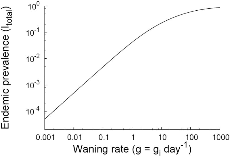
A plot of the fraction of the population infected at equilibrium for measles parameter values. The horizontal axis varies the waning rate g in the special case where the waning rates between all compartments are equal (g_i = g for all i). In contrast to Figure 2, there are no parameter regions with multiple equilibria.

5 Discussion

Individuals can acquire many differing degrees of immunity from an immune response to an infectious disease. But until now, there has been little systematic analysis of the consequences of the structure of acquired immunity for the dynamics of disease transmission at the population level. In this paper, we first introduced a general model for structured acquired immunity. The model was then specified further with some biologically motivated assumptions: that both risk of infection and duration of infection decrease as immunity increases; that infection does not decrease immunity; and that immune waning causes a sequential decrease in immune state, i.e. from state i to state i − 1. Together these assumptions are referred to as the Immunity Dynamics Hypothesis (IDH), which we believe to be a reasonable first guess about structured immunity for a particular pathogen in the absence of specific information to the contrary.

Under the IDH, structured immunity alone can not create backward bifurcations in a simple epidemic model; the disease-free equilibrium is the only equilibrium for R₀ < 1. However, for R₀ > 1, multiple equilibria can exist (e.g. Figure 2). Theorems 2 and 3 give sufficient conditions for uniqueness of the stable equilibrium for R₀ > 1, although the biological interpretation of these conditions remains unclear.

This work suggests that epidemic models exhibiting bistability for R₀ < 1 do not do so solely because of immunity; other effects are needed. In our previous paper (Reluga and Medlock, 2007), we indicated how behavior changes can introduce bistability. Strong demographic effects can also introduce bistability. For example, Corbett et al. (2003) study a model where contact rate is independent of population size, and shows that disease-induced mortality creates a backward bifurcation by rapidly shrinking the population. Dushoff (1996) also presents a model that can have a backward bifurcation, in this case when the severity of infection is positively correlated to the force of infection, as may happen with some macroparasite infections.

The IDH is not an appropriate hypothesis for immunity in all situations. If infection makes subsequent re-infection more likely, the IDH does not hold. For example, it has been suggested that infection with some strains of human papillomavirus may make infection with other strains more likely (Thomas et al., 2000; Liaw et al., 2001; Rousseau et al., 2001). In these circumstances, the interaction between pathogen and host immunity can result in bistability for R₀ < 1 (i.e. a backward bifurcation) due to the presence of the pathogen in the population improving conditions for its own dissemination. Age-dependent effects on immunity can be important for childhood diseases, and transient memory dynamics in the immune system can be important for periodic epidemics like influenza. In addition, the IDH requires that greater immunity shortens the duration of infection, while it is possible that greater immunity leads to a longer but less severe infection.

Even when the IDH does hold, there are pathogens, like measles in the presented data, for which the dynamics of acquired immunity violate Theorems 2 and 3. In simulation studies of vaccine-acquired resistance to influenza, Smith et al. (1999) suggest that antibody cross-reactivity from older strains may hinder the acquisition of resistance to new strains. While vaccination always increases individual resistance, completely naive individuals may have greater resistance to a new strain after exposure than individuals who were already partially resistant. If so, this violates Theorem 3, as in our example, System 3.24 (see Figure 2). Thus, influenza dynamics could exhibit multiple equilibria for R₀ > 1. Another possibility is illustrated in the dengue modeling of Cummings et al. (2005), where the transmission rate of an infective person increases in a person’s second infection. This process could cause a backward bifurcation since the presence of the pathogen in the host population improves conditions for its own dissemination. More examples are needed to determine if multiple equilibria can be created by immunity in real populations or if they are an artifact of unrealistic parameter choices.

Several open problems remain in this work. There is clearly still room to strengthen Theorem 3 and to find better biological interpretations of our results. Of particular importance, our results need to be extended to specifically incorporate vaccination events. The extension of System (2.2) to include vaccination would, in general, require the introduction of a second immunity kernel satisfying constraints similar to those imposed by the IDH. We expect that Theorem 1 should continue to hold under vaccination conditions, but it is not yet clear how far Theorems 2 and 3 can be extended. Besides incorporating vaccination, work is needed to account for transmission rates that depend on the immunity level of an infected individual. Generalization of these results to models with a continuum of immunity levels, using partial-differential-equation analogs of System (2.2) like the one studied by Martcheva and Pilyugin (2006), would also be valuable. Systematic determinations of the local and global stability of the stationary solutions are also needed.

The model and analysis presented here suggest that under our common expectations, immunity does not dramatically change the dynamics of simple SIS models. Similar models might be helpful in examining strain interactions, timing of outbreaks, and many other epidemiological phenomena.

A Proof of Theorem 3

Proof

A sufficient differential condition for S_j(I_Total) to be stochastically decreasing is that for every k,

$$\frac{\mathrm{d}}{\mathrm{d}{I}_{\mathrm{Total}}}\sum _{j=1}^k{S}_j=(1-I_{\mathrm{Total}})\frac{\mathrm{d}}{\mathrm{d}{I}_{\mathrm{Total}}}\frac{{\sum }_{j=1}^k{x}_j}{{\sum }_{j=1}^n{x}_j}-\frac{{\sum }_{j=1}^k{x}_j}{{\sum }_{j=1}^n{x}_j}$$ (A.1a)

$$\le \frac{\mathrm{d}}{\mathrm{d}{I}_{\mathrm{Total}}}\frac{{\sum }_{j=1}^k{x}_j}{{\sum }_{j=1}^n{x}_j}$$ (A.1b)

$$=\frac{{\sum }_{j=1}^k{x}_j^{\prime }{\sum }_{j=1}^n{x}_j-{\sum }_{j=1}^k{x}_j{\sum }_{j=1}^n{x}_j^{\prime }}{{\left({\sum }_{j=1}^n{x}_j\right)}^2}$$ (A.1c)

$$=\frac{{\sum }_{i=1}^k{\sum }_{j=k+1}^n\left(x_i^{\prime }{x}_j-x_i{x}_j^{\prime }\right)}{{\left({\sum }_{j=1}^n{x}_j\right)}^2},$$ (A1.d)

where ′ denotes the derivative with respect to I_Total. Now the elasticity of x_j is

$$E_j=\frac{I_{\mathrm{Total}}}{x_j}{x}_j^{\prime }.$$ (A.2)

Since x₁ = 1, $x_1^{\prime }=0$ and the first elasticity E₁ = 0. x₂ is proportional to I_Total, so E₂ = 1. In terms of elasticities,

$$x_i^{\prime }{x}_j-x_i{x}_j^{\prime }=\frac{x_i{x}_j}{I_{\mathrm{Total}}}(E_i-E_j).$$ (A.3)

If the elasticities are monotone increasing over the index j, i.e. E_j ≤ E_j+1 for all j, then

$$\frac{{\sum }_{i=1}^k{\sum }_{j=k+1}^n\left(x_i^{\prime }{x}_j-x_i{x}_j^{\prime }\right)}{{\left({\sum }_{j=1}^n{x}_j\right)}^2}=\frac{{\sum }_{i=1}^k{\sum }_{j=k+1}^n{x}_i{x}_j(E_i-E_j)/I_{\mathrm{Total}}}{{\left({\sum }_{j=1}^n{x}_j\right)}^2}\le 0.$$ (A.4)

So it will suffice to prove that the elasticities E_j are increasing.

To construct the elasticities explicitly, we return to Eq. (3.12). To simplify the algebra, let

$$H_{\mathit{ik}}=1-\sum _{j=1}^k{f}_{\mathit{ij}}=\sum _{j=k+1}^n{f}_{\mathit{ij}}$$ (A.5)

so that

$$x_{k+1}=\frac{\beta I_{\mathrm{Total}}}{g_{k+1}}\sum _{i=1}^k{\sigma }_i{x}_i{H}_{\mathit{ik}}.$$ (A.6)

Note that 0 ≤ H_ik ≤ 1, but it is only defined for I ≤ k. Now, the elasticity

$$\begin{array}{ll}{E}_{k+1}=\frac{I_{\mathrm{Total}}}{x_{k+1}}{x}_{k+1}^{\prime }& =1+I_{\mathrm{Total}}\frac{{\sum }_{i=1}^k{\sigma }_i{x}_i^{\prime }{H}_{\mathit{ik}}}{{\sum }_{i=1}^k{\sigma }_i{x}_i{H}_{\mathit{ik}}}\\ & =1+\frac{{\sum }_{i=1}^k{\sigma }_i{E}_i{x}_i{H}_{\mathit{ik}}}{{\sum }_{i=1}^k{\sigma }_i{x}_i{H}_{\mathit{ik}}}.\end{array}$$ (A.7)

Since all the terms are non-negative, it follows that E₃ ≥ E₂.

We proceed with a proof by induction. Given E_m+1 ≥ E_m for all m < k, prove E_k+1 ≥ E_k. Well,

$$E_{k+1}-E_k=\frac{{\sum }_{j=1}^k{\sigma }_j{E}_j{x}_j{H}_{jk}}{{\sum }_{j=1}^k{\sigma }_j{x}_j{H}_{\mathit{jk}}}-\frac{{\sum }_{i=1}^{k-1}{\sigma }_i{E}_i{x}_i{H}_{i,k-1}}{{\sum }_{i=1}^{k-1}{\sigma }_i{x}_i{H}_{i,k-1}}$$ (A.8a)

$$=\frac{{\sum }_{i=1}^{k-1}{\sum }_{j=1}^k{\sigma }_i{x}_i{H}_{i,k-1}{\sigma }_j{x}_j{H}_{jk}(E_j-E_i)}{{\sum }_{i=1}^{k-1}{\sum }_{j=1}^k{\sigma }_i{x}_i{H}_{i,k-1}{\sigma }_j{x}_j{H}_{\mathit{jk}}}$$ (A.8b)

$$=\frac{{\sum }_{i=1}^{k-1}{\sum }_{j=i+1}^k{\sigma }_i{x}_i{\sigma }_j{x}_j(H_{i,k-1}{H}_{\mathit{jk}}-H_{j,k-1}{H}_{\mathit{ik}})(E_j-E_i)}{{\sum }_{i=1}^{k-1}{\sum }_{j=1}^k{\sigma }_i{x}_i{H}_{i,k-1}{\sigma }_j{x}_j{H}_{jk}}$$ (A.8c)

where we define H_k,_k−1 = 0. Under the induction assumption, the first k elasticities are increasing, so j > i implies E_j − E_i is non-negative. If follows that E_k+1 − E_k ≥ 0 so long as

$$H_{i,k-1}{H}_{\mathit{jk}}-H_{j,k-1}{H}_{\mathit{ik}}=$$ (A.9a)

$$(\sum _{l=k}^n{f}_{\mathit{il}})\left(\sum _{l=k+1}^n{f}_{\mathit{jl}}\right)-(\sum _{l=k}^n{f}_{\mathit{jl}})\left(\sum _{l=k+1}^n{f}_{\mathit{il}}\right)=$$ (A.9b)

$$f_{\mathit{ik}}(\sum _{l=k+1}^n{f}_{\mathit{jl}})-f_{\mathit{jk}}\left(\sum _{l=k+1}^n{f}_{\mathit{il}}\right)=$$ (A.9c)

$$f_{\mathit{ik}}(\sum _{l=k}^n{f}_{\mathit{jl}})-f_{\mathit{jk}}(\sum _{l=k}^n{f}_{\mathit{il}})\ge 0$$ (A.9d)

for all i < j ≤ k or, equivalently, for i = j − 1 and all j ≤ k.

References

- 1.Amanna IJ, Carlson NE, Slifka MK. Duration of humoral immunity to common viral and vaccine antigens. New England Journal of Medicine. 2007;357(19):1903–1915. doi: 10.1056/NEJMoa066092. [DOI] [PubMed] [Google Scholar]
- 2.Anderson RM, May RM. Infectious Diseases of Humans: Dynamics and Control. Oxford University Press; New York, NY: 1991. [Google Scholar]
- 3.Arino J, McCluskey CC, van den Driessche P. Global results for an epidemic model with vaccination that exhibits backward bifurcations. SIAM Journal of Applied Mathematics. 2003;64(1):260–276. [Google Scholar]
- 4.Bayas JM, Vilella A, Bertran MJ, Vidal J, Batalla J, Asenjo MA, Salleras LL. Immunogenicity and reactogenicity of the adult tetanus–diphtheria vaccine. How many doses are necessary? Epidemiology and Infection. 2002;127(03):451–460. doi: 10.1017/s095026880100629x. [DOI] [PMC free article] [PubMed] [Google Scholar]
- 5.Bin D, Chen ZH, Liu QC, Wu T, Guo CY, Wang XZ, Fang HH, Xiang YZ. Duration of immunity following immunization with live measles-vaccine - 15 years of observation in Zhejiang province, China. Bulletin of the World Health Organization. 1991;69(1):415–423. [PMC free article] [PubMed] [Google Scholar]
- 6.Boldin B. Introducing a population into a steady community: The critical case, the center manifold, and the direction of bifurcation. SIAM Journal on Applied Mathematics. 2006;66(1):1424–1453. [Google Scholar]
- 7.Broliden K, Abreu ER, Arneborn M, Bottiger M. Immunity to mumps before and after MMR vaccination at 12 years of age in the first generation offered the two-dose immunization programme. Vaccine. 1998;16(23):323–7. doi: 10.1016/s0264-410x(97)88332-6. [DOI] [PubMed] [Google Scholar]
- 8.Corbett BD, Moghadas SM, Gumel AB. Subthreshold domain of bistable equilibria for a model of HIV epidemiology. International Journal of Mathematics and Mathematical Sciences. 2003;58:3679–3698. [Google Scholar]
- 9.Cummings DAT, Schwartz IB, Billings L, Shaw LB, Burke DS. Dynamic effects of antibody-dependent enhancement on the fitness of viruses. Proceedings of the National Academy of Sciences of the United States of America. 2005;102(42):15259–15264. doi: 10.1073/pnas.0507320102. [DOI] [PMC free article] [PubMed] [Google Scholar]
- 10.Dushoff J. Incorporating immunological ideas in epidemiological models. Journal of Theoretical Biology. 1996;180(1):181–187. doi: 10.1006/jtbi.1996.0094. [DOI] [PubMed] [Google Scholar]
- 11.Feng ZL, Castillo-Chavez C, Capurro AF. A model for tuberculosis with exogenous reinfection. Theoretical Population Biology. 2000;57(1):235–247. doi: 10.1006/tpbi.2000.1451. [DOI] [PubMed] [Google Scholar]
- 12.Gomes MGM, Margheri A, Medley GF, Rebelo C. Dynamical behaviour of epidemiological models with sub-optimal immunity and nonlinear incidence. Journal of Mathematical Biology. 2005;51(1):414–430. doi: 10.1007/s00285-005-0331-9. [DOI] [PubMed] [Google Scholar]
- 13.Govaert T, Sprenger M, Dinant G, Aretz K, Masurel N, Knottnerus J. Immune response to influenza vaccination of elderly people. A randomized double-blind placebo-controlled trial. Vaccine. 1994;12(13):1185–9. doi: 10.1016/0264-410x(94)90241-0. [DOI] [PubMed] [Google Scholar]
- 14.Homann D, Teyton L, Oldstone MB. Differential regulation of antiviral T-cell immunity results in stable CD8+ but declining CD4+ T-cell memory. Nature Medicine. 2001;7(8) doi: 10.1038/90950. [DOI] [PubMed] [Google Scholar]
- 15.Kribs-Zaleta CM, Velasco-Hernandez JX. A simple vaccination model with multiple endemic states. Mathematical Biosciences. 2000;164:183–201. doi: 10.1016/s0025-5564(00)00003-1. [DOI] [PubMed] [Google Scholar]
- 16.Kuby J. Immunology. W. H. Freeman and Company; New York, NY: 1994. [Google Scholar]
- 17.Lee MS, Nokes DJ, Hsu HM, Lu CF. Protective titres of measles neutralising antibody. Journal of Medical Virology. 2000;62(1):511–517. doi: 10.1002/1096-9071(200012)62:4<511::aid-jmv17>3.0.co;2-z. [DOI] [PubMed] [Google Scholar]
- 18.Liaw K-L, Hildesheim A, Burk R, Gravitt P, Wacholder S, Manos M, Scott D, Sherman M, Kurman R, Glass A, Anderson S, Schiffman M. A prospective study of human papillomavirus (HPV) type 16 DNA detection by polymerase chain reaction and its association with acquisition and persistence of other HPV types. Journal of Infectious Diseases. 2001;183(1):8–15. doi: 10.1086/317638. [DOI] [PubMed] [Google Scholar]
- 19.Lipsitch M, Murray MB. Multiple equilibria: Tuberculosis transmission require unrealistic assumptions. Theoretical Population Biology. 2003;63(2):169–170. doi: 10.1016/s0040-5809(02)00037-0. [DOI] [PubMed] [Google Scholar]
- 20.Macdonald G. The analysis of equilibrium in malaria. Tropical Diseases Bulletin. 1952;49(9):813–29. [PubMed] [Google Scholar]
- 21.Martcheva M, Pilyugin S. An epidemic model structured by host immunity. Journal of Biological Systems. 2006;14(2):185–203. [Google Scholar]
- 22.May RM, Gupta S, McLean AR. Infectious disease dynamics: What characterizes a successful invader. Philosophical Transactions of the Royal Society of London. 2001;356:901–910. doi: 10.1098/rstb.2001.0866. [DOI] [PMC free article] [PubMed] [Google Scholar]
- 23.Reluga T, Medlock J. Resistance mechanisms matter in SIRS models. Mathematical Biosciences and Engineering. 2007 July;4(3):553–563. doi: 10.3934/mbe.2007.4.553. [DOI] [PubMed] [Google Scholar]
- 24.Rousseau M-C, Pereira J, Prado J, Villa L, Rohan T, Franco E. Cervical coinfection with human papillomavirus (HPV) types as a predictor of acquisition and persistence of HPV infection. Journal of Infectious Diseases. 2001;184(12):1508–1517. doi: 10.1086/324579. [DOI] [PubMed] [Google Scholar]
- 25.Smith DJ, Forrest S, Ackley DH, Perelson AS. Variable efficacy of repeated annual influenza vaccination. Proceedings of the National Academy of Sciences of the United States of America. 1999 November 23;96(24):14001–14006. doi: 10.1073/pnas.96.24.14001. [DOI] [PMC free article] [PubMed] [Google Scholar]
- 26.Thomas K, Hughes J, Kuypers J, Kiviat N, Lee S-K, Adam D, Koutsky L. Concurrent and sequential acquisition of different genital human papillomavirus types. Journal of Infectious Diseases. 2000;182(4):1097–1102. doi: 10.1086/315805. [DOI] [PubMed] [Google Scholar]