Language processing with dynamic fields

Abstract

We construct a mapping from complex recursive linguistic data structures to spherical wave functions using Smolensky’s filler/role bindings and tensor product representations. Syntactic language processing is then described by the transient evolution of these spherical patterns whose amplitudes are governed by nonlinear order parameter equations. Implications of the model in terms of brain wave dynamics are indicated.

Electronic supplementary material

The online version of this article (doi: 10.1007/s11571-008-9042-4) contains supplementary material, which is available to authorized users.

Introduction

Human language processing is accompanied by modulations of the ongoing electrophysiological brain waves. If these are evaluated in a stimulus-locked manner (cf. the contributions of Fründ et al. and Kiebel et al. in this special issue), one speaks about event-related brain potentials that reflect syntactic (Osterhout and Holcomb 1992; Friederici 1995), semantic (Kutas and Hillyard 1980, 1984) and also pragmatic (Noveck and Posada 2003; Drenhaus et al. 2006) processing problems.

Modeling human language processing has previously relied mostly upon computational approaches from automata theory and cognitive architectures (Hopcroft and Ullman 1979; Lewis and Vasishth 2006), while dynamical system models that could also be able to account for brain wave dynamics are still in their infancy (beim Graben et al. 2008; Vosse and Kempen 2000; Garagnani et al. 2007). The contentious issues of the former approach regarding the computational viability of grammars intended to capture properties of human language have been with us since Chomsky (1957). The nature of this long debate centers around whether the models of language and language processing proposed are, in principle, computable; computability being a minimal requirement for any attempt to formally describe complex behavior exhibited by a biological system. As our understanding of the biology and physiology of the brain has increased, similar issues have guided the development of computational models of brain physiology. There are now interesting competing models for both language processes (Elman 1995; Tabor et al. 1997; Christiansen and Chater 1999; Vosse and Kempen 2000; beim Graben et al. 2008; Hagoort 2005; Lewis and Vasishth 2006; van der Velde and de Kamps 2006; Smolensky and Legendre 2006) and brain functions (Wilson and Cowan 1973; Amari 1977; Jirsa and Haken 1996; Coombes et al. 2003; Jirsa 2004; Wright et al. 2004; Garagnani et al. 2007) (see also the contributions in this special issue).

Although language understanding takes place in the human brain, computational modeling of language processes and computational modeling of brain physiology are not the same. The models address quite different levels of description and reflect different assumptions regarding the operational primitives and desired final states. While the former generally refer to abstract feature spaces such as “stack tapes”, “neural blackboards” or “sketch pads” (Hopcroft and Ullman 1979; Anderson 1995; van der Velde and de Kamps 2006), the latter aim at describing membranes, neurons, or mass potentials (beim Graben 2008). Nevertheless, a successful model of language processing should be interpretable in terms of a model of brain function. This represents a new kind of evaluative paradigm on models of language or more generally cognitive processes: (1) Is the model computationally tractable? (2) Is the model interpretable in terms of descriptions of the supporting physiology?

Following this approach, computational models of language processing must take very seriously the properties inherent in computational models of the brain. In doing so we are led to address the issues and assumptions raised by the differing levels of description targeted by the models. We are also provided with a metric for comparison of competing models.

Here we address the question: Can the basic assumptions and mechanisms underpinning a language processing model be expressed in terms that are compatible with viable models of the brain? Our answer will be yes, and furthermore, we argue that this result has direct bearing on important debates regarding the viability of certain classes of language processing models.

An outstanding controversial issue is whether grammars and processing mechanisms of human languages are recursive or not (Hauser et al. 2002; Everett 2005) and whether neural network models should implement this property either faithfully or rather by means of graceful saturation (Christiansen 1992; Christiansen and Chater 1999; Smolensky 1990; Smolensky and Legendre 2006). Especially Smolensky’s Integrated Connectionist/Symbolic architecture (Smolensky and Legendre 2006; Smolensky 2006) represents symbolically meaningful states by very few very sparse patterns in very high, yet finite, dimensional activation vector spaces (beim Graben et al. 2007, 2008).

In order to avoid such sparse representations, we suggest employing infinite-dimensional function spaces in this paper. This approach is in line with related attempts by Smolensky (1990), Moore and Crutchfield (2000), Maye and Werning (2004), Werning and Maye (2007) and compatible with neural and dynamical field theories of cognition (Wilson and Cowan 1973; Amari 1977; Jirsa and Haken 1996; Coombes et al. 2003; Jirsa 2004; Wright et al. 2004; Erlhagen and Schöner 2002; Schöner and Thelen 2006; Thelen et al. 2001).

We shall construct a mapping from the dynamics of language processing into a field dynamics in several steps. First, in Section “Dynamic parsing”, we describe a simplified parsing dynamics based upon a toy-grammar, to be introduced in Section “Grammars”. Second, in Section “Fock space representations”, we shall study a particular vector space representation of phrase structure trees as suggested by Smolensky (1990) and Smolensky and Legendre (2006). We also embed the time-discrete representation of the parsing process into a time-continuous dynamics. In Section “Order parameter dynamics” we derive neurally motivated order parameter equations (Haken 1983) of the parser. Third, in Section “Spherical wave functions”, we map the vectorial representation of the parsing states into the function space of spherical harmonics defined on an abstract feature space. Here, the crucial point is to reduce the dimension of the vector space by a separation of time scales. Finally, the different parts of the model are integrated into a field-theoretic representation with transient dynamics in Section “Dynamic fields”. Section “Simulations” presents results of numerical simulations of the parsing example discussed throughout the paper. We conclude with a discussion about a tentative relation between our model and electrophysiological findings on language-related brain waves.

Grammars

Sentences are hierarchically structured objects, commonly described by phrase structure trees in linguistics (Chomsky 1957; Hopcroft and Ullman 1979). Contemporary linguistic and parsing theories have elaborated considerably on these early approaches (cf. Stabler 1997 for one particular account). For our purposes, we investigate a toy-grammar that simplifies our task but is nevertheless representative of the basic operations required of a natural language parser.

Consider e.g. the sentence

Example 1

This simple sentence consists of a subject, the noun phrase and a predicate, the verbal phrase The latter in turn is construed from the verb and another noun phrase, the direct object Therefore, the sentence from example 1 can be described by the tree depicted in Fig. 1.

Fig. 1.

Phrase structure tree of the sentence

From the phrase structure tree in Fig. 1, a context-free grammar (CFG) can be easily derived by taking the node as the start symbol and as another nonterminal such that every branching of the tree corresponds to a production of the grammar with

1

where is a finite terminal alphabet, is a finite set of nonterminal categories, comprises the production rules, and is the distinguished start symbol.

The productions p ∈  P are usually drawn as rule expansions

2

as in (1), where and γ is a finite word of the Kleene hull (Hopcroft and Ullman 1979). We call a production pbinary branching, if i.e. γ in (2) is a word of length 2, γ = v₁v₂, with Accordingly, we call a CFG G binary branching, if all rules p ∈ P are binary branching. Obviously, our example grammar G is binary branching.

Dynamic parsing

In order to understand a sentence the brain has to recognize at least “who is doing what to whom?” (Bornkessel et al. 2005), i.e, it has to reconstruct the phrase structure tree from the sequence of words. This mapping from a sentence to a tree is called parsing. Context-free languages can be parsed through push-down automata (Hopcroft and Ullman 1979). The simplest of these devices, the top-down recognizer, emulates the so-called left-derivation of a phrase structure tree, where always the leftmost not yet expanded nonterminal is expanded according to the rules of the grammar (1). Starting with the start symbol we can thus derive the following strings:

3

Binary branching CFGs give rise to labeled binary phrase structure trees by successively expanding rules from P through left-derivations as in Fig. 1. Figure 2 shows the evolution of the phrase structure trees for the sentence according to grammar (1).

Fig. 2.

Left-derivation (3) of the sentence according to grammar (1)

Figure 2 reveals parsing as a dynamics in the space of phrase structure trees (Kempson et al. 2001). Formally, we define: Let T be the set of binary labeled phrase structure trees consistent with a given binary branching context-free grammar G. Clearly, T contains the “tree” (the start symbol at the root) and at least one tree s for each well-formed sentence. A mapping

4

is a sequential dynamic top-down parser if the following holds: There is a constant such that for all

1. is a subtree of s of height l,

2. π expands the tree s as a left-derivation,

3. 

We call L the duration of the parsing process. The parse of s generated by π is the trajectory

5

which is a “word” of length L in the Kleen hull T^*.

Fock space representations

In this section, we present a mathematically rigorous reconstruction of the tensor product representations that have been introduced by Smolensky (1990, 2006), Smolensky and Legendre (2006) and further supported by Mizraji (1989, 1992).

Let S be a set of symbolic structures, e.g., of feature lists (Stabler 1997) or of phrase structure trees (i.e. S = T) (Chomsky 1957; Hopcroft and Ullman 1979). How can we represent a structured expression s ∈ S by a vector in some vector space? We follow Smolensky by introducing two finite sets F and R of elementary fillers and elementary roles, respectively.

Consider e.g. the set of binary labeled trees T for the CFG G (1) as an example. Let s ∈ T be the tree in Fig. 2c. First, we have to chose fillers and roles. A suitable choice for the elementary fillers are the variables of G, i.e. The elementary roles are the three positions as indicated in Fig. 3.

Fig. 3.

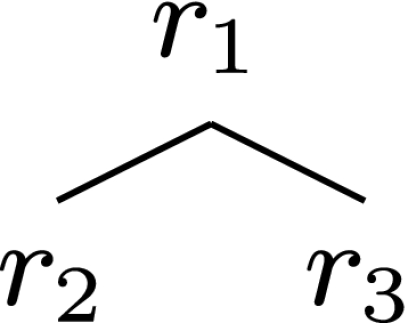
Elementary role positions of a labeled binary tree

A filler/role binding for a basic building block of s, denoted f/r, is an ordered pair (f, r) ∈ F × R. Decomposing s into a set of (elementary) filler/role bindings yields a subset f′ = {(f_i, r_j) | i ∈ I, j ∈ J} (I, J are particular index sets) of F × R. The set f′ is therefore an element of the power set

6

where denotes the set of all subsets of a set X.

In our example, we first bind the elementary fillers to r₁, to r₂ and to r₃, obtaining the complex filler

Next, recursion comes into the game. The subsets f′ of F × R are complex fillers that can in turn bind to other roles: f′/r. This again is an ordered pair belonging to the next-level filler/role binding f′′ = {(f′_i, r_j) | i ∈ I′, j ∈ J′}. Therefore

7

Looking at the tree Fig. 2c in our example, reveals that the complex filler is recursively bound to tree position r₃ at the higher level, whereas the elementary fillers and are attached to r₁ and r₂, respectively. Thus, the tree s ∈T is mapped onto its filler/role binding

8

For even higher trees, we have to repeat this construction recursively, entailing a hierarchy of filler/role bindings

9

In this way, any finite structure s ∈ S becomes decomposed into its filler/role bindings by a map

10

for a particular In order to deal with recursion properly, we further define the collection

11

After decomposing the structure s into its filler/role bindings, β(s), we map s onto a vector from a vector space by the tensor product representation ψ, obeying

1. 

2. ψ(F_n) is a subspace of for all in particular for F₀ = F is a subspace of

3. is a subspace of

4. for all f ∈ F_n, r ∈ R,

5. for all substructures s_i of s ∈S.

Taken together, these properties yield that is the Fock space

12

known from quantum field theory (Haag 1992).

In order to apply the tensor product representation to our example CFG G (1) with phrase structure trees T, we identify the categories of G with their associated filler vectors ψ(f). On the other hand, we represent the roles with the “one-particle” Fock space basis

13

This notation has the advantage, that both, the tensor products in item 4, and the direct sums in item 5, , can be omitted, simply writing ψ(f_i) |r_j〉, and respectively.

The tree s in (8) is than mapped onto the Fock space vector

14

where we wrote the tensor products as “two-particle” Fock space vectors |ij〉.

Now, we are able to map a parse, namely a trajectory of trees U ∈ T^* generated by a sequential dynamic top-down parser π (5) onto a trajectory of Fock space vectors

15

Correspondingly, the parser π is represented by a nonlinear operator

16

defined through

17

for all x ∈ T belonging to a parse U.

For our example above, the Fock space representation of the parse U shown in (3) and in Fig. 2, is obtained as

18

In Section “Dynamic fields”, we are going to describe the Fock space parser P_π by a dynamically evolving field. A suitable function space for these fields will be constructed in Section “Spherical wave functions”. To this aim, we need an embedding of the time-discrete dynamics (15) into continuous time. We achieve this construction by an order parameter expansion (Haken 1983) of the form

19

where the time-dependent coefficient λ_l(t) is the order parameter for the lth subtree of the parse U. Each order parameter λ_l(t) assumes a unique maximum at time when the lth tree has been established. Accordingly, T_L denotes the duration of the whole parse in continuous time. The functions λ_l(t) form a Lagrange basis with λ_l(T_k) = A_kδ_lk and A_k the amplitude of the k-th order parameter (Kress 1998, Chap. 8)

The order parameter dynamics is usually governed by order parameter equations

20

with appropriate functions g_l (Haken 1983).

Order parameter dynamics

We will discuss two different approaches to determine the time evolution of the coefficients λ_l(t), l = 0,…, L and The first approach will be based on a simple recursion formula leading to a partition of unity for the coefficients. The second approach is build on order parameter dynamics as suggested by Haken (1983). Here, we will incorporate the neural background of our mapping and use a system of coupled nonlinear differential equations based on a leaky integrator neuron model.

Dynamics based on a recursion formula

For our recursive dynamics we start with some function δ₀ shaping the decay dynamics of the our coefficients. Here, the constant denotes the maximal time interval on which a coefficient is active. For this first approach this means that λ_l(t) > 0. Later we will also work with coefficients which are not compactly supported, then activation is more complex and might be understood as the period in time in which the coefficient superseeds some threshold.

We assume that δ₀ is monotonic and continuous on δ₀(0) = 1 and Also, we define δ₁ = 1−δ₀ on which yields δ₁(0) = 0 and Now, we set

21

Then, we define the coefficients λ_l for l ≥ 1 by

22

The functions λ_l build a partition of unity, i.e. we have the property

23

Further, the support of the coefficient λ_l is a subset of

Neural order parameter dynamics

Basically, Eq. 20 is a leaky integrator equation that is often used in neural modeling (beim Graben and Kurths 2008; beim Graben 2008). It can also be seen as a discretized version of the Amari equation for neural/dynamical fields (Wilson and Cowan 1973; Amari 1977; Jirsa and Haken 1996; Coombes et al. 2003; Jirsa 2004; Wright et al. 2004; Erlhagen and Schöner 2002; Schöner and Thelen 2006; Thelen et al. 2001). Thus it is promising to relate (20) with brain dynamics.

Since each well-established parse state s_l at time T_l triggers its successor s_l+1, we choose a similar delay ansatz for the coupling functions g_l in (20) as in Section “Dynamics based on a recursion formula”:

24

25

for t ≥ 0.

Here, the sigmoidal logistic functionf with cut constant η and spread parameter σ is defined by

26

and w, η, σ and τ_l = τ are real positive constants. For the case σ = 0 we use the jump function

27

which corresponds to the limit of f_η,σ for σ → ∞. The properties of the solutions to (20)–(27) depend strongly on σ. For σ = 0 it has singular points, for σ > 0 it is a smooth function.

Spherical wave functions

Let be the n-dimensional space spanned by the (linearly independent) filler vectors and be the 3-dimensional space spanned by the “one-particle” roles (13).

Our approach relies upon a separation ansatz where the fillers are described by functions of time, while the roles are given by spherical harmonics at the unit sphere S. First, we identify the n fillers with functions f_k(t).

Next, we regard the tree in Fig. 3 as a “deformed” term schema for a spin-one triplet (Fig. 4).

Fig. 4.

Tree roles in a spin-one term schema

Figure 4 indicates that the three role positions |1〉, |2〉, |3〉 in a labeled binary tree have been identified with the three z-projections of a spin-one particle:

28

which have an L²(S) representation by spherical harmonics

29

In order to deal with complex phrase structure trees, we have to describe the tensor products of role vectors Inserting the spin eigenvectors from (28), yields expressions like

30

well-known from the spin coupling in quantum mechanics (Edmonds 1957).

In quantum mechanics, the product states (30) generally belong to different multiplets, which are given by the irreducible representations of the spin algebra sl(2). These are obtained by the Clebsch–Gordan coefficients in the expansions

31

where the total angular momentum j obeys the triangle relation

32

However, our aim appears to be a bit different. Instead of computing the state of the coupled system by means of (31), we have to express the particular state vector (30) through higher harmonic wave functions. Therefore, we have to invert (31), leading to

33

with the constraint m = m₁ + m₂.

Equation (33) has to be applied recursively in order to obtain the role positions of more and more complex phrase structure trees. Finally, a single tree s ∈ T is represented by its filler/role bindings in the basis of spherical harmonics

34

where the coefficients a_jkm = 0 if filler k is not bound to pattern Y_jm. Otherwise, the a_jkm encode the Clebsch–Gordan coefficients in Eq. (33).

Combining (34) with the order parameter ansatz (19), yields the spatio-temporal parsing dynamics

35

indicating a separation of time scales (Haken 1983): the fast functions f_k(t) in s_l(φ, ϑ, t) encode instantaneous trees, while the transient evolution of the order parameters λ_l(t) reflects the time course of the parsing process.

Let us illustrate this construction in the light of our example CFG G (1). The five fillers are encoded by functions f_k(t) with k = 1, 2,…, 5.

The first state, of the parse (18) in Fock space is simply given by

since For the second state, we straightforwardly obtain the representation

Only computing the third and final state, turns out to be somewhat cumbersome. In a first step, we get

Expressing the tensor products by (33), yields firstly

The first Clebsch–Gordan coefficient 〈0, 1, 1, 1 | 1, 0, 1, 1〉 = 0 because a spin j = 0 particle cannot have an m = 1 projection. On the other hand, the Clebsch–Gordan coefficients are and

Correspondingly, we obtain for

Here, m = 0 is consistent with j = 0, 1, 2 such that all three terms have to be taken into account through and

Finally, we consider

Obviously, only the last term contributes to the sum with 〈2, 2, 1, 1 | 1, 1, 1, 1〉 = 1 for the same reason as above.

Summarizing, the parse U in Fig. 2, possessing the abstract Fock space representation (18), translates into the time-discrete dynamics

36

Dynamic fields

Dynamic field theories (DFT) are a phenomenological account for continuum models in the cognitive sciences (Erlhagen and Schöner 2002; Schöner and Thelen 2006; Thelen et al. 2001). They are mathematically equivalent to neural field theories (Wilson and Cowan 1973; Amari 1977; Jirsa and Haken 1996; Coombes et al. 2003; Jirsa 2004; Wright et al. 2004; beim Graben 2008), yet not referring to a particular neurophysiological description but rather to dynamics in abstract feature space.

In order to obtain such dynamic fields, we bring (36) together with (35) to generate the time-continuous parsing dynamics:

37

In order to complete our description, we have to determine the filler functions f_k(t) in (37). One possible choice is to assign eigenfrequencies

38

to the five fillers such that the fillers become represented as harmonic oscillations

39

in time.

Then, the parse U in Fig. 2, possessing the Fock space representation (37), translates into

40

Simulations

The stationary waves representing the three parse steps s₀, s₁ and s₂ of in (36) are shown in Fig. 5(a–c) as a sequence of snapshots, respectively.1

Fig. 5.

Snapshot sequences of the moduli of the stationary waves |s₁| (36). (a) for the initial state s₀, (b) for s₁, (c) for s₂

Note that the initial state s₀ is given by the constant “p_z orbital” (Fig. 5a).

In the representation of s₁ we have a superposition of the constant function from s₀ with two higher harmonics, indicating the fillers f₂(t) and f₃(t) assigned to the tree position roles r₃ and r₂, respectively (Fig. 5b). The final state s₂ is given by an even more involved oscillation (Fig. 5c).

Additionally, we present in Fig. 6. the dynamics of |s₁| (Fig. 5b) with higher temporal resolution.

Fig. 6.

Snapshot sequence of the state |s₁| with higher temporal resolution

Now, the first column of Fig. 6. corresponds to the first six images in the row of Fig. 5b; the toroidal dynamics accounted for by the fillers f₂(t) and f₃(t) is clearly visible.

Figure 7 displays the temporal evolution of the three order parameters λ_l(t), denoting the amplitudes of the corresponding parse states s_l, according to the order parameter equation (20) with the coupling functions g_l (24). For the numerical simulation of the neural order parameter equation we used Euler’s method (Kress 1998, Chap. 10).

Fig. 7.

Dynamics of the three order parameters λ₀(t) (solid), λ₁(t) (dashed-dotted), and λ₂(t) (dotted), generated via (20)–(27). (a) for σ = 0, (b) for σ = 10. The calculations have been carried out with the parameter choices η = 0.5 and delay time

Figure 7 reveals that the parse states s₀, s₁, and s₂ are fully established at times T₀ ≈ 50, T₁ ≈ 150, and T₂ ≈ 250, where the order parameters assume their respective local maxima.

Finally, Fig. 8 presents the transient evolution of the dynamic parse field according to (40) as a sequence of snapshots.

Fig. 8.

Snapshot sequence of the dynamic field |u| representing the transient evolution of the parse in Fock space

Comparing Fig. 8 with Fig. 5 shows that the parse states s₀, s₁, and s₂ become established at times T₀ ≈ 50, T₁ ≈ 150, and T₁ ≈ 250 in accordance with Fig. 7.

Discussion

In Section “Introduction” we have raised the question: Can the basic assumptions and mechanisms underpinning a language processing model be expressed in terms that are compatible with viable models of the brain? The basic assumptions and mechanisms of linguistics are that symbolic expressions are complex and recursive hierarchical data structures which are symbolically processed by appropriate cognitive architectures (Chomsky 1957; Hopcroft and Ullman 1979; Lewis and Vasishth 2006). On the other hand, macroscopic brain function is often modeled in terms of neural field dynamics (Wilson and Cowan 1973; Amari 1977; Jirsa and Haken 1996; Coombes et al. 2003; Jirsa 2004; Wright et al. 2004; Erlhagen and Schöner 2002; Schöner and Thelen 2006; Thelen et al. 2001).

In order to respond to that question, we have constructed a faithful mapping from linguistic phrase structure trees to the infinite-dimensional function space of spherical wave functions, using Smolensky’s filler/role bindings and tensor product representations (Smolensky 1990, 2006; Smolensky and Legendre 2006). The abstract feature space of this representation is the unit sphere S. Language processing is than described by the transient evolution of spherical patterns, governed by order parameter equations for their respective amplitudes (Haken 1983). For the order parameter equations we chose a neural leaky integrator model with delayed coupling between the parse states.

Since spherical harmonics are also often employed in analyzing electroencephalographic brain waves (Nunez and Srinivasan 2006), it is tempting to simply identify the feature space S of our model with a spherical head model, thereby interpreting the dynamic field u(φ, ϑ, t) of the parser with the actual voltage distribution across the human scalp. However, such a straightforward interpretation is not tenable as it would require the whole brain to be in only a few representative states necessary to maintain one particular cognitive task. This is obviously not the case. Therefore we would need another mapping from the abstract feature space representation of our model to a neural representation in the brain in order to answer the question in the end. We shall leave this issue for future research on the cognitive neurodynamics of brain waves.

References

- Amari SI (1977) Dynamics of pattern formation in lateral-inhibition type neural fields. Biol Cybern 27:77–87 [DOI] [PubMed]
- Anderson JR (1995) Cognitive psychology and its implications, 4th edn. W. H. Freeman and Company, New York
- beim Graben P (2008) Foundations of neurophysics. In: beim Graben P, Zhou C, Thiel M, Kurths J (eds) Lectures in supercomputational neuroscience: dynamics in complex brain networks. Springer Complexity Series. Springer, Berlin, pp 3–48
- beim Graben P, Kurths J (2008) Simulating global properties of electroencephalograms with minimal random neural networks. Neurocomputing 71(4):999–1007 [DOI]
- beim Graben P, Gerth S, Saddy D, Potthast R (2007) Fock space representations in neural field theories. In: Biggs N, Bonnet-Bendhia AS, Chamberlain P, Chandler-Wilde S, Cohen G, Haddar H, Joly P, Langdon S, Lunéville E, Pelloni B, Potherat D, Potthast R (eds) Proceedings of Waves 2007. The 8th international conference on mathematical and numerical aspects of waves. Department of Mathematics, University of Reading, Reading, pp 120–122
- beim Graben P, Gerth S, Vasishth S (2008) Towards dynamical system models of language-related brain potentials. Cogn Neurodynam. doi:10.1007/s11571-008-9041-5 [DOI] [PMC free article] [PubMed]
- Bornkessel I, Zysset S, Friederici AD, von Cramon DY, Schlesewsky M (2005) Who did what to whom? The neural basis of argument hierarchies during language comprehension. NeuroImage 26:221–233 [DOI] [PubMed]
- Chomsky N (1957) Syntactic structures. Mouton, Den Haag
- Christiansen MH (1992) The (non)necessity of recursion in natural language processing. In: Proceedings of the 14th annual conference on Cognitive Science Society, Lawrence Erlbaum Associates, Hillsdale, pp 665–670
- Christiansen MH, Chater N (1999) Toward a connectionist model of recursion in human linguistic performance. Cogn Sci 23(4):157–205 [DOI]
- Coombes S, Lord G, Owen M (2003) Waves and bumps in neuronal networks with axo-dendritic synaptic interactions. Physica D 178:219–241 [DOI]
- Drenhaus H, beim Graben P, Saddy D, Frisch S (2006) Diagnosis and repair of negative polarity constructions in the light of symbolic resonance analysis. Brain Lang 96(3):255–268 [DOI] [PubMed]
- Edmonds AR (1957) Angular momentum in quantum mechanics. Princeton University Press, Princeton
- Elman JL (1995) Language as a dynamical system. In: Port RF, van Gelder T (eds) Mind as motion: explorations in the dynamics of cognition. MIT Press, Cambridge, pp 195–223
- Erlhagen W, Schöner G (2002) Dynamic field theory of movement preparation. Psychol Rev 109(3):545–572 [DOI] [PubMed]
- Everett DL (2005) Cultural constraints on grammar and cognition in Pirahã – another look at the design features of human language. Curr Anthropol 46(4):621–646 [DOI]
- Friederici AD (1995) The time course of syntactic activation during language processing: a model based on neuropsychological and neurophysiological data. Brain Lang 50:259–281 [DOI] [PubMed]
- Garagnani M, Wennekers T, Pulvermuller F (2007) A neuronal model of the language cortex. Neurocomputing 70:1914–1919 [DOI]
- Haag R (1992) Local quantum physics: fields, particles, algebras. Springer, Berlin
- Hagoort P (2005) On Broca, brain, and binding: a new framework. Trends Cogn Sci 9(9):416–423 [DOI] [PubMed]
- Haken H (1983) Synergetics. An introduction, Springer series in synergetics, vol 1, 3rd edn. Springer, Berlin. 1st edition 1977
- Hauser MD, Chomsky N, Fitch WT (2002) The faculty of language: What is it, who has it, and how did it evolve? Science 298:1569–1579 [DOI] [PubMed]
- Hopcroft JE, Ullman JD (1979) Introduction to automata theory, languages, and computation. Addison–Wesley, Menlo Park
- Jirsa VK (2004) Information processing in brain and behavior displayed in large-scale scalp topographies such as EEG and MEG. Int J Bifurcat Chaos 14(2):679–692 [DOI]
- Jirsa VK, Haken H (1996) Field theory of electromagnetic brain activity. Phys Rev Lett 77(5):960–963 [DOI] [PubMed]
- Kempson R, Meyer-Viol W, Gabbay D (2001) Dynamic syntax. The flow of language understanding. Blackwell
- Kress R (1998) Numerical analysis, graduate texts in mathematics, vol 181. Springer-Verlag, New York
- Kutas M, Hillyard SA (1980) Reading senseless sentences: brain potentials reflect semantic incongruity. Science 207:203–205 [DOI] [PubMed]
- Kutas M, Hillyard SA (1984) Brain potentials during reading reflect word expectancy and semantic association. Nature 307:161–163 [DOI] [PubMed]
- Lewis RL, Vasishth S (2006) An activation-based model of sentence processing as skilled memory retrieval. Cogn Sci 29:375–419 [DOI] [PubMed]
- Maye A, Werning M (2004) Temporal binding of non-uniform objects. Neurocomputing 58:941–948 [DOI]
- Mizraji E (1989) Context-dependent associations in linear distributed memories. Bull Math Biol 51(2):195–205 [DOI] [PubMed]
- Mizraji E (1992) Vector logics: the matrix-vector representation of logical calculus. Fuzzy Sets Syst 50:179–185 [DOI]
- Moore C, Crutchfield JP (2000) Quantum automata and quantum grammars. Theor Comput Sci 237:275–306 [DOI]
- Noveck IA, Posada A (2003) Characterizing the time course of an implicature: an evoked potentials study. Brain Lang 85:203–210 [DOI] [PubMed]
- Nunez PL, Srinivasan R (2006) Electric fields of the brain: the neurophysics of EEG. Oxford University Press, New York
- Osterhout L, Holcomb PJ (1992) Event-related brain potentials elicited by syntactic anomaly. J Mem Lang 31:785–806 [DOI]
- Schöner G, Thelen E (2006) Using dynamic field theory to rethink infant habituation. Psychol Rev 113(2):273–299 [DOI] [PubMed]
- Smolensky P (1990) Tensor product variable binding and the representation of symbolic structures in connectionist systems. Artif Intell 46:159–216 [DOI]
- Smolensky P (2006) Harmony in linguistic cognition. Cogn Sci 30:779–801 [DOI] [PubMed]
- Smolensky P, Legendre G (2006) The harmonic mind. From neural computation to optimality-theoretic grammar, vol 1: cognitive architecture. MIT Press, Cambridge
- Stabler EP (1997) Derivational minimalism. In: Retoré C (ed) Logical aspects of comutational linguistics, Springer Lecture Notes in Computer Science, vol 1328. Springer, New York, pp 68–95
- Tabor W, Juliano C, Tanenhaus MK (1997) Parsing in a dynamical system: an attractor-based account of the interaction of lexical and structural constraints in sentence processing. Lang Cogn Process 12(2/3):211–271
- Thelen E, Schöner G, Scheier C, Smith LB (2001) The dynamics of embodiment: A field theory of infant perseverative reaching. Behav Brain Sci 24:1–86 [DOI] [PubMed]
- van der Velde F, de Kamps M (2006) Neural blackboard architectures of combinatorial structures in cognition. Behav Brain Sci 29:37–108 [DOI] [PubMed]
- Vosse T, Kempen G (2000) Syntactic structure assembly in human parsing: a computational model based on competitive inhibition and a lexicalist grammar. Cognition 75:105–143 [DOI] [PubMed]
- Werning M, Maye A (2007) The cortical implementation of complex attribute and substance concepts: synchony, frames, and hierarchical binding. Chaos Complex Lett 2(2/3):435–452
- Wilson HR, Cowan JD (1973) A mathematical theory of the functional dynamics of cortical and thalamic nervous tissue. Kybernetik 13:55–80 [DOI] [PubMed]
- Wright JJ, Rennie CJ, Lees GJ, Robinson PA, Bourke PD, Chapman CL, Gordon E, Rowe DL (2004) Simulated electrocortical activity at microscopic, mesoscopic and global scales. Int J Bifurcat Chaos 14(2):853–872 [DOI] [PubMed]
Associated Data
This section collects any data citations, data availability statements, or supplementary materials included in this article.
Supplementary Materials
Below is the link to the electronic supplementary material.