Graphical-model-based Multivariate Analysis of Functional Magnetic Resonance Data

Abstract

We propose a method for the analysis of functional magnetic resonance (fMR) data, based on a Bayesian-network representation. Our method identifies multivariate linear/nonlinear voxel-activation pattern differences across groups, which may provide information complementary to that resulting from a general linear model (GLM)-based analysis. In addition, we describe a model-stabilization method based on data resampling, which may be helpful in the presence of small numbers of subjects, or when data are noisy.

1 Introduction

Many functional magnetic-resonance (fMR) studies center on finding activation differences among different groups, such as normal elderly vs. demented elderly (Buckner et al. (2000)), normal females vs. females with fragile-X syndrome (Tamm et al. (2002)), or reading Chinese characters versus Pinyin (Chen et al. (2002)). Most of these fMR studies examine functional segregation (Lazar et al. (2002); Worsley et al. (2002); Penny et al. (2003)), i.e., they examine a hypothesis in which a particular cortical area is specialized for some aspect of cognition. Evaluation of these hypotheses typically proceeds in two steps: within-subject analysis, to detect activated voxels for a single subject, followed by between-subject analysis, to determine activation-pattern differences among experimental groups. In this context, we denote by F the categorical group-membership variable; for the sake of simplicity, we refer to F as the clinical variable.

Methods for between-subject analysis are often mass univariate, and adopt the general linear model (GLM) framework. Most commonly, random-effects analysis (Penny et al. (2003)) is performed; in this approach, differences of observed effects are assumed to be due to a combination of data noise and between-subject variability. For example, using the SPM analysis application, (The Wellcome Department of Imaging, Institute of Neurology, University College London), a contrast image is computed for each subject, and GLM-based methods, such as the t-test or analysis of variance, are used to detect differences among these contrast images.

Although widely applied, mass-univariate statistical analysis of fMR data to characterize group differences has important limitations. First, as typically implemented, GLM-based methods incorporate the assumption that voxel activations are consistent for subjects in the same group, and that intersubject variability within an experimental group is due to noise. Second, GLM-based methods can detect linear associations among voxel activation and F, but are not designed to detect nonlinear associations.

To highlight these limitations, assume that we are studying two groups of subjects performing the same task; group 1 is the experimental group, and group 2 consists of normal control subjects. Consider three scenarios, as depicted in Figure 1. In scenario 1 (Figure 1, top), for the experimental group, region A and only A is consistently activated in the task, and subjects in the normal control group manifest consistent activation in a brain region other than A. In this case, a GLM-based mass-univariate method will identify region A as characterizing group differences.

Figure 1.

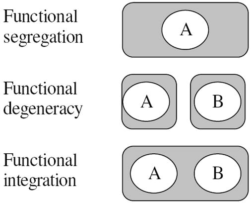
An illustration of functional segregation, degeneracy, and integration. Each gray rectangle represents a task, the rectangle contains brain regions (white ellipses) required to complete that task.

In scenario 2 (Figure 1, middle), control subjects manifest consistent activation in a brain region other than A or B. However, subjects in the experimental group engage two different sub-processes. Some of them engage a sub-process dependent only on region A; others engage a sub-process dependent only on region B. This scenario is an example of functional degeneracy (Edelman and Gally (2001); Price and Friston (2002); Noppeney et al. (2006)), defined as “the ability of elements that are structurally different to perform the same function or yield the same output” (Edelman and Gally (2001)). An example of functional degeneracy is seen when examining action retrieval. Phillips et al. suggested that an action for an object is retrieved either from visual structural features or from accessing semantic knowledge (Phillips et al. (2002)). GLM-based approaches cannot distinguish regions related to different sub-processes in the presence of functional degeneracy.

In the third scenario (Figure 1, bottom), subjects in both the experimental and control groups engage a process dependent on both A and B—an example of functional integration (Friston (1994)). Assume further that the association among F and regions A and B is nonlinear, for example, an exclusive-OR (XOR) function. GLM-based methods cannot handle this type of nonlinear structure-function association, because, considered individually, neither A nor B manifests an activation difference between experimental and control groups.

To facilitate the detection of regions characterizing group differences in case of functional degeneracy or nonlinear associations among regions and the clinical variable, we propose a novel approach, called functional graphical-model-based multivariate analysis (fGAMMA). The major strength of fGAMMA is that it models multivariate associations among voxel-activation patterns and F, based on a Bayesian-network (BN) representation (Pearl (1988)).

As we described in Section 2.2, there are two major advantages to using Bayesian networks, rather than GLM-based approaches, to model associations among brain regions and F: (1) a BN can represent linear or nonlinear associations among variables of interest; in fact, a BN can represent any joint distribution of categorical variables; and (2) a BN is a probabilistic model that encodes uncertainty, which could include data noise, experimental error, and uncertainty regarding cognitive processes.

Although the primary goal of our approach is to identify associations among voxel-activation patterns and F, it is important to identify a model that is stable under data perturbation, because a fMR study may involve small number of subjects, rendering the resulting model unstable to data noise. Therefore, we employ an ensemble-learning approach to stabilize the model. The rationale behind ensemble methods is to reduce model variability via averaging (Breiman (1996); Freund and Schapire (1996); Breiman (2001)).

The remainder of this paper is organized as follows: Section 2 describes fMR data preprocessing, within-subject analysis, Bayesian networks, and an overview of fGAMMA. We present experimental results in Section 3. Section 4 consists of discussion and conclusions.

2 Methods

Figure 2 provides an overview of data flow within the fGAMMA framework. First, fMR images undergo preprocessing, to generate binary-voxel activation maps. Next, fGAMMA generates Bayesian-network model of associations among voxel variables and F, and a corresponding label field, in which each voxel is labeled as belonging to a cluster, or region of interest; this process may be embedded within a model-aggregation resampling framework, to evaluate how stable the Bayesian-network model is to data noise.

Figure 2.

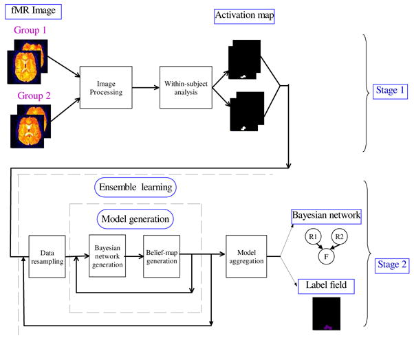
An overview of the analysis procedure

2.1 fMR data preprocessing and within-subject analysis

We used SPM2 for data preprocessing (Figure 2, Stage 1). First, we aligned the images within an acquisition, normalized them to the MNI space, and then smoothed the normalized images using a 9mm-FWHM isotropic Gaussian kernel.

We also used SPM2 to perform within-subject analysis, that is, to detect the activation foci for a single subject (Friston et al. (1995)). We used a high-pass filter with a cut-off period of 128 seconds to remove low-frequency noise, and we used an AR(1) model to correct for serial correlation in the temporal domain. Statistics comparing the estimated effects with appropriate error measures were generated; these results constitute statistical parametric maps for each contrast of interest. Finally, we chose a p-value with family-wise error correction to threshold the statistical parametric maps; for each analysis, we chose this parameter from the typical range of p-value [0.001, 0.05] ¹. Thresholding yielded a binary effect map, whose voxels assume states in {0, 1}, representing off (no effect) and on (effect) at each voxel, respectively. If the contrast of interest represents voxel activation, we herein refer to the generated effect map as a binary activation map.

2.2 Bayesian network

We use Bayesian networks to model multivariate associations among voxel-activation patterns and F. A Bayesian network is a probabilistic graphical model defined as = { , Θ}; and Θ are defined presently. The structure of the Bayesian network, = { , }, is a directed acyclic graph (DAG), where = {X₁, X_2,…, X_n} represents the variables in to be analyzed, and is a set of edges representing associations among these variables. If X_i→X_j is an edge in , then X_i is called a parent node of X_j. We use pa(X_j) to denote the set of parents of X_j.

To quantify probabilistic associations among variables in a BN, we specify the conditional-probability distribution P(X_i | pa(X_i)). If the variables are continuous, the commonly used model assumes P(X_i | pa(X_i)) is Gaussian, implying that the joint distribution of {X_i} be multivariate Gaussian, which may be too restrictive for our application. To enable fGAMMA to detect nonlinear multivariate associations among voxel variables and F, we employ the discrete Bayesian network, in which all variables are categorical, to model this domain. In this case, when we assume that P(X_i | pa(X_i)) is an unrestricted multinomial distribution, the corresponding BN can represent any joint distribution among these variables.

Each variable X_i in a BN is associated with a conditional-probability table, which represents p(X_i | pa(X_i)). Let θ_ijk = p(X_i = k | pa(X_i) = j) be the conditional probability of X_i assuming state k, given that its parents, pa(X_i), assume joint state j; if X_i does not have parents, then θ_i·k = p(X_i = k) is a marginal distribution. Θ = {θ_ijk} constitutes the parameters of the BN.

An example of a simple BN is depicted in Figure 3. In this BN, pa(F) = {A, B}, and p(F = 1 | A = 1, B = 0) = 0.9 means that the probability of a subject’s being in group 1, given that region A is activated and region B is not, is 0.9.

Figure 3.

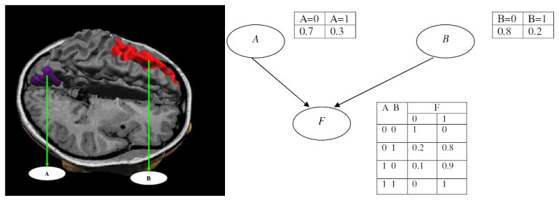
An example of a fMR study. Left: brain regions involved. Right: a Bayesian network that represents probabilistic associations among regions A and B, and the clinical variable F.

Since the number of potential BN models increases exponentially in the number of variables, in our implementation we restricted the type of BN model in fGAMMA to have inverse-tree structure, as shown in Figure 4. In a Bayesian network with inverse-tree structure, F is a leaf node and all other variables (for fGAMMA, all fMR voxel variables) are parents of F.

Figure 4.

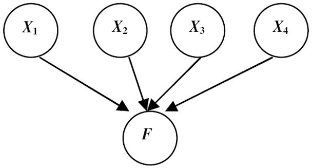
A Bayesian network with inverse-tree structure

A common approach to BN generation from a data set D is to define a metric that captures the fidelity of a BN model to associations among variables in D, as well as the parsimony of that model; this metric guides the search for ∗, the model that optimizes this metric. The most widely used metric is the BDe score (Herskovits (1991); Cooper and Herskovits (1992); Heckerman et al. (1995)); derivation of the BDe score is based on the assumptions that each variable X_i (1 ≤ i ≤ n) in is discrete, that X_i assumes a state in {1, 2,…, r_i}, where r_i is the number of states that X_i can assume (e.g., 2 for a binary variable), and that, for fixed structure , the prior distribution of Θ is Dirichlet: P(θ_ij1,…, θ_ijri | ) ~ Di(α_ij1,…, α_ijri). Given these assumptions, the BDe score, P (D | ), can be expressed as

$$P(\mathbf{D}\mid \mathcal{S})=\prod _{i=1}^n\prod _{j=1}^{q_i}\frac{\mathrm{\Gamma }({\alpha }_{ij})}{\mathrm{\Gamma }({\alpha }_{ij}+N_{ij})}\prod _{k=1}^{r_i}\frac{\mathrm{\Gamma }({\alpha }_{\mathit{ijk}}+N_{\mathit{ijk}})}{\mathrm{\Gamma }({\alpha }_{\mathit{ijk}})},$$ (1)

where N_ijk is the the number of samples in D for which X_i = k and pa(X_i) = j; q_i is the number of states pa(X_i) can assume; N_ij = ∑_k N_ijk; and α_ij = ∑_k α_ijk. Note that BDe metric, which does not distinguish among categorical variable states; that is, this score is invariant to inversion of all variables, or, in general, remapping of states of multinomial variables.

Given a fixed structure, the posterior distribution of P(θ_ij1,…, θ_ijri | ) is Dirichlet Di(α_ij1+N_ij1, …, θ_ijri+N_ijri). The maximum a posterior estimation of parameters Θ are as follows:

$${\widehat{\theta }}_{\mathit{ijk}}=\frac{N_{\mathit{ijk}}+{\alpha }_{\mathit{ijk}}}{N_{ij}+{\alpha }_{ij}}.$$ (2)

θ̂_ijk is the mean of posterior distribution. The variance of posterior which is

$$\frac{(N_{\mathit{ijk}}+{\alpha }_{\mathit{ijk}})(N_{ij}+{\alpha }_{ij}-N_{\mathit{ijk}}-{\alpha }_{\mathit{ijk}})}{{(N_{ij}+{\alpha }_{ij})}^2(N_{ij}+{\alpha }_{ij}+1)}$$ (3)

can be used to describe the uncertainty in estimate θ_ijk (Gelman et al. (1995)).

2.3 Functional Graphical-model-based Multivariate Analysis

As stated in the previous section, fGAMMA generates a Bayesian network with inverse-tree structure; in this network, which F is the leaf node, and each parent of F represents a ROI, or collection of voxels manifesting a common activation pattern. A key property of fGAMMA is that each ROI is among those most strongly associated with F.

Figure 5 explains how the generated Bayesian network distinguishes among subjects in different experimental groups. Assume that several regions are involved in performing a task (e.g., regions 1–6 in Figure 5(a)); we can model the associations among these regions and F using a Bayesian network (Figure 5(b)). However, exhaustive search for the optimal Bayesian network is intractable, due to the sheer number of possible models. To solve this problem, we exploit a key property of Bayesian networks: conditional independence. Let I(X; Y | Z) represent the statement that X and Y are conditionally independent, given Z. Given a set of variables , which includes X and Y, the Markov blanket of X is defined as the smallest set in that renders X conditionally independent of Y, that is, I(X; Y | mb(X)) for all Y ∈ \{X, mb(X)} (Pearl (1988); Koller and Sahami (1996)). In other words, given knowledge of the variables in mb(F), knowledge of any other variables in tells us nothing more about F, and thus will not increase predictive accuracy. Note that mb(F) for a Bayesian network with inverse-tree structure is simply the parent set of F. We previously proved that the set of the parents of F in a Bayesian network with inverse-tree structure (Figure 5 (c)) is guaranteed to be a subset of mb(F) in the ground-truth Bayesian network (Figure 5(b)) (Chen and Herskovits (2005a)). Therefore, the ROIs generated by fGAMMA are among those that are most informative about F.

Figure 5.

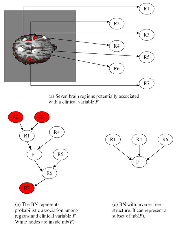
A hypothetical demonstration of how fGAMMA is designed to generate a Bayesian network characterizing group differences; note that Markov blankets in inverse-tree models are subsets of those in unrestricted Bayesian networks.

Let be the set of all voxels defined in the standard MNI space. In the BN-generation process, fGAMMA identifies a subset of voxels RV = {RV_1,…, RV_l} in that are jointly informative about F. Belief-map generation constructs, for each RV_i, a ROI consisting of voxels that are probabilistically equivalent to RV_i. By probabilistically equivalent, we mean that two voxels tend to be in the same state across subjects and experimental conditions. Finally, in the model-aggregation step, fGAMMA checks for statistical artifacts, and modifies the BN model to obtain a stable model.

As previously described in Section 2.1, within-subject analysis for each subject i yields a binary effect map D_i. Let D = {D₁, D₂,…,D_M} and F = {F₁, F₂,…, F_M}, where M is the total number of subjects in the study. We provide the image data D and clinical variable F as input to fGAMMA.

2.3.1 Bayesian-network generation

fGAMMA iteratively performs BN generation and belief-map generation: BN generation yields a small set of representative voxels, whose activation states are strongly associated with F, and belief-map generation yields a set of probabilistically equivalent voxels for each representative voxel; groups of probabilistically equivalent voxels constitute clusters of voxels that have similar probabilistic associations with F. Note that a particular cluster may not be spatially contiguous.

The overall goal of Bayesian-network generation is to select representative voxels that are strongly associated with F. In particular, fGAMMA searches for the representative-voxel set, RV^*= {RV₁, RV₂,…,RV_l}, that maximizes the BDe score for the BN in which pa(F) = RV^*. That is,

$$\mathbf{R}{\mathbf{V}}^{\ast }=\underset{\mathbf{R}\mathbf{V}}{\text{argmax}}\mathit{BDe}(\mathcal{S},\mathbf{D}),$$ (4)

where is an inverse-tree structure, and pa(F) = RV in .

Let denote the entire voxel set. As the computational cost of exhaustive search over all possible RV sets grows exponentially with the number of voxels in , exhaustive search is infeasible for a nontrivial data set. Instead, fGAMMA employs heuristic search to find RV*. Let RV_k and V_k be the representative voxel set and the set of all candidate voxels in iteration k, respectively. fGAMMA starts with an empty representative voxel set RV₀, V₀ = , and iteration index k = 0. On iteration k + 1, fGAMMA first computes the BDe score for the BN structure with pa(F) = RV_k, denoted by BDe(RV_k); then we calculate BDe(RV_k ∪ {V_i}) for V_i in V_k, and add it to a candidate set A if Δ(V_i) = BDe(RV_k ∪ {V_i}) − BDe(RV_k) > 0. Within A, we search for the voxel that maximizes Δ(V_i), and we assign that voxel to RV_k+1. That is,

$$R{V}_{k+1}=\underset{V_i:V_i\in \mathbf{A}}{\text{argmax}}\mathrm{\Delta }(V_i).$$ (5)

The next step is to identify a set of voxels, E ⊂ V_k, that are probabilistically equivalent to RV_k+1. We describe the details of this step, including our definition of probabilistic equivalence, in the next paragraph. Finally, we add the new representative voxel to the representative voxel set (RV_k+1 ← RV_k ∪ {RV_k+1}), we remove the new representative voxel and all voxels that are equivalent to it from the candidate voxel set (V_k+1 ← V_k \{{RV_k+1} ∪ E}), we increment k, and proceed to the next iteration. The model-generation process ends when A = ∅ or V_k+1 = ∅.

2.3.2 Belief-map generation

Belief-map generation identifies a set of ROIs; each ROI consists of a representative voxel and all voxels that are probabilistically equivalent to it. We define a voxel X as probabilistically equivalent to voxel Y if their probabilistic associations with F, that is, their conditional-probability distributions, are similar. For binary X and Y, one measure of probabilistic equivalence is P(X = 0, Y = 1) ≈ 0 and P(X = 1, Y = 0) ≈ 0. In iteration k, fGAMMA’s belief-map generation algorithm searches voxels in A rather than in V_k−1 to generate the equivalence set E, because Δ(RV_k) > 0, and A consists of all voxels V_i in V_k−1 for which Δ(V_i) > 0. Restricting the search space to A instead of V_k−1 can greatly reduce search time and the false-positive rate, since A is typically a small subset of V_k−1.

For each voxel V_i in the candidate set A, fGAMMA calculates the equivalence metric s(V_i, RV_k )= P (V_i = 1, RV_k = 1) + P(V_i = 0, RV_k = 0) to define probabilistic equivalence. The similarity map, S = {s(V₁, RV_k), …, s(V_l, RV_k )}(V_i ∈ A), constitutes the input to belief-map generation. We treat as a clustering problem the task of inferring the equivalence set E for RV_k, based on the similarity map S. We previously implemented a contextual-clustering algorithm to solve this problem (Chen and Herskovits (2005b)).

We refer to the mean similarity measure of voxels within each cluster as the centroid of that cluster. fGAMMA identifies the cluster with the largest centroid, and thus the greatest similarity measure, as the equivalence set for RV_k. This process labels each voxel with its equivalence-set membership. Let L_i be the label variable associated with the voxel at location i. L = {L₁, L₂, …, L_a} represents the label set, where a is the number of voxels in A.

To incorporate spatial information, we model the prior for L as a pairwise Markov random field (MRF). In particular, we employ a MRF with a second-order neighborhood system defined on a 3D lattice, as shown in Figure 6. For any voxel location i, the Markov blanket of i, denoted by mb(i), consists of voxel locations associated with nonzero potential functions. Because in-plane resolution usually exceeds z-axis resolution for fMR experiments, we assume that interactions among voxels in the x – y plane are stronger than those in the z direction, and therefore that mb(i) consists of the eight surrounding locations in the x – y plane, and the two locations directly above and below i in the z direction, as shown in Figure 6. However, an fGAMMA user can specify any neighborhood type for the MRF.

Figure 6.

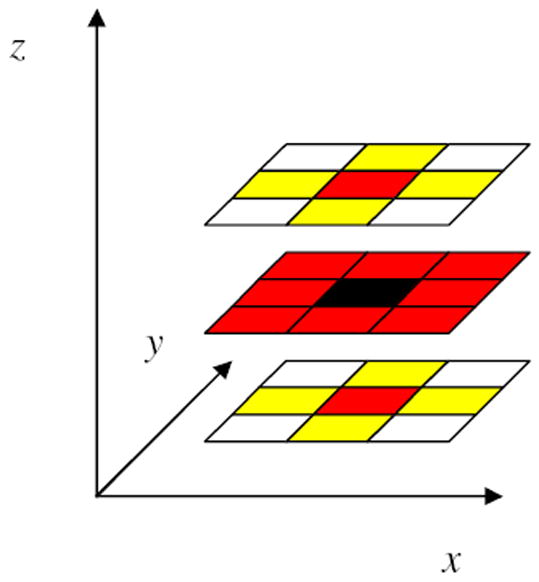
A second-order neighborhood system in a 3D lattice. The yellow and red voxels are the neighbors of the black voxel. The red voxels constitute the Markov blanket of the black voxel.

Let c be the number of clusters in the label map L (1 ≤ c ≤ a). ϒ = {μ₁, μ₂,…, μ_c} is the set of centroids. Given c, the goal is to find L̂ and ϒ̂, such that

$$\{\widehat{\mathbf{L}},\widehat{\mathrm{\Upsilon }}\}=\underset{\mathbf{L},\mathrm{\Upsilon }}{\text{argmax}}P(\mathbf{L},\mathrm{\Upsilon }\mid \mathbf{S}).$$ (6)

L̂ and ϒ̂ are the MAP estimation of L and ϒ, given S. We use a generalized expectation-maximization (EM) method to solve this problem; this algorithm iteratively searches for L and ϒ. In iteration k, our approach first finds L̂(k) that maximizes P(L | S, ϒ̂ (k − 1)); then searches for ϒ̂ (k) that maximizes P(ϒ | S, L̂(k)). Finding ϒ̂(k) is straightforward: when L̂(k) is known, for all voxels in the same cluster based on L̂(k), the empirical mean of intensities in the similarity map is the best linear unbiased estimator of μ.

Given ϒ̂, the maximum a posteriori (MAP) estimate of L is

$$\widehat{\mathbf{L}}=\underset{\mathbf{L}}{\text{argmax}}\prod _{i,j}\psi (L_i,L_j)\prod _i\phi (L_i,S_i),$$ (7)

where S_i = s(V_i, RV_k); ψ(L_i, L_j) = e^{−β(μ(i) −μ(j))2} and φ(L_i, S_i) = e^{−(Si−μ(i))2}; i ∈ A and j ∈ mb(i). μ(i) is the centroid of the cluster to which voxel i belongs. β is a parameter controlling smoothness.

We use loopy belief propagation (Weiss (1997); Yedidia et al. (2003)) to find the MAP estimate of L. The output of loopy belief propagation for each voxel is a vector with length c, whose values constitute the probability distribution for this voxel’s membership in each cluster. We choose the mode of this distribution, which we call L̂_i, to be the label for voxel location i. We present further details regarding Equation 7, the estimation of c, and loopy belief propagation in the Appendix.

In this manner, the label field Λ stores probabilistic-equivalence. Let N_r be the cardinality of RV; then Λ contains N_r ROIs {C₁, C₂, …, C_Nr}, each ROI consisting of a representative voxel and its equivalent voxels. For voxel V_i, if, based on L̂_i, this voxel is probabilistically equivalent to representative voxel RV_k, we set the value of this voxel in Λ to k; if a voxel is not equivalent to any representative voxel, we set its value in the label field to 0. Each cluster in Λ thus constitutes a ROI in which voxels are considered homogeneous with respect to their probabilistic association with F, as represented by the conditional probability distribution P(RV_k | F).

2.3.3 Model aggregation

Bayesian-network generation and belief-map generation yield a model = ( , Λ), where and Λ represent a Bayesian network and a label field, respectively. However, the model generated from D, which consists of the activation maps for all subjects, may not be stable under data perturbation, for two reasons. First, a fMR study comparing groups or trial conditions may include a small number (e.g., dozens) of subjects, whereas the cardinality of the hypothesis space , from which we select the model, is an exponential function of the number of voxels. In this model-generation problem, if we have N voxels in the stereotaxic space, and if we set the maximum length of RV to be r, then the size of the hypothesis space, | |, is ${\sum }_{k=1}^r\left(\begin{array}{c}N\\ k\end{array}\right)$. For N = 10000 and r = 3, | |> 10¹¹. Due to the sheer size of H, there could exist many models with the same BDe score. Second, Bayesian-network generation is based on greedy search, which may cause fGAMMA to be sensitive to small perturbations of D.

We therefore implemented a model-aggregation algorithm to increase the stability of our results in the face of noise, undersampling, and heuristic search. This algorithm selects different subsets of D, generates a model for each subset, and aggregates the resulting models. Let the training samples be D = {D₁, …, D_M}, where M is the total number of subjects and D_i is the activation map for subject i. We use the jackknife method to generate a subset of samples Dⁱ = {D₁, …, D_i−1, D_i+1, …, D_M}, in which we exclude the activation map for subject i. For each Dⁱ, we generate a model = ( , Λⁱ). We thus obtain a model ensemble: Ξ = { }. We induce a stabilized model by aggregating models in the ensemble Ξ.

Algorithm 1 delineates this model-aggregation process; D constitutes the input. Steps 1 and 2 generate a model ensemble Ξ. In step 3, we calculate the frequency of model pattern j, defined as

Algorithm 1.

Model aggregation in fGAMMA

1: Remove the ith sample from D to generate Di (1 ≤ i ≤ M);

2: Generate a model = ( , Λi) for each Di;

3: Calculate the frequency of model based on { };

4: Select the mode of ;

5: for each class j in do

6:  Calculate the class map based on {Λk | = };

7:   Threshold to get a binary class map;

8: end for

$$f_{\mathcal{B}}(j)=\sum _{i=1}^M{1}_{[{\mathcal{B}}^i={\mathcal{B}}^j]},$$ (8)

where 1_[cond] is an identity function, equal to 1 if cond is true, 0 otherwise; and is the histogram of model occurrence for { }. In the next step we select the mode of , , because is the most stable BN among { }. is associated with a set of models, { }, whose = .

Since all {Λ^k} are associated with , their representative voxel sets must also be identical. However, the values of voxels in Λ^k may differ among these models, because fGAMMA uses different data sets Dⁱ to compute Λ^k for each model. Therefore, we must aggregate these {Λ^k}; this process is shown in steps 5–8. To reconcile these differences, we create a class map for each representative voxel RV_a associated with . Each voxel in the class map is the probability of that voxel’s belonging to class a, defined as:

$$V_{\mathcal{C}}(i)=\frac{{\sum }_{j=1}^{N_r}{1}_{[{\mathrm{\Lambda }}_i^j=a]}}{N_r},$$ (9)

where N_r is the cardinality of set {Λ^k}, and ${\mathrm{\Lambda }}_i^j$ denote voxel i in label field Λ^j. Finally, we assign a class to each voxel by voting. If a voxel is in class a for the majority of subjects in { }, we set that voxel in Λ^mode to a. The output of Algorithm 1 is an aggregated model ∗ = ( , Λ^mode).

3 Experimental results

In this section, we apply fGAMMA to synthetic data, and to data from a previously published study including young, and nondemented and demented older adults.

3.1 Simulated Data

In this experiment, we synthesized fMR data for 24 subjects, based on data from a visual-motor experiment available with Voxbo software (http://www.voxbo.org/). Each subject was presented with flashing lights, and either performed sequential finger tapping or rested, in eight 42-second alternating blocks. The 14 volumes in each block were acquired 3 seconds apart; there were thus a total of 112 volumes. Image size was 64 × 64 × 45, and spatial resolution was 3 × 3 × 3 mm³. For each subject, we generated a binary activation map, corresponding to each voxel’s activation state. The activation regions included bilateral motor and visual areas.

We synthesized a study with two groups of 24 subjects each. Subjects in group 2 were exposed to a stimulus, whereas those in group 1 were not. In generating the data for group 2, we stipulated that exactly one of two regions, A and B, with equal probability, would be activated when a subject was exposed to the stimulus; that is, either region A or region B would be activated, but not both. This is a typical functional degeneracy scenario. In this manner, we generated 12 subjects with [A = 1, B = 0, F = 2] and 12 subjects with [A = 0, B = 1, F = 2], where [A = 1, B = 0, F = 2] represents a subject with activation of region A, no activation of region B, and membership in group 2.

In the MNI space, we created two bounding-boxes: bounding-box 1 incorporated right and left visual areas, and bounding-box 2 contained right and left motor areas. We used the binary activation map of the visual areas in the Voxbo data set as the activation map for region A, and that of the motor areas in the Voxbo data set as the activation map for region B. Let D^simu(i) and D^voxbo(i) represent the activation map of subject i in simulated data and in Voxbo data, respectively. We initialized D^simu(i) to zero at each voxel. For group 1, we created 24 activation-difference maps with all zero values, representing [A = 0, B = 0, F = 1]. For each of the 12 samples of type [A = 1, B = 0, F = 2], region A was activated and B was not; since A = 1, for voxels in the bounding-box 1, we set their values in D^simu(i) to be same as those in D^voxbo(i). Since B = 0, for voxels in bounding-box 2, their values in D^simu(i) remained zero. We performed a similar procedure to generate 12 samples of type [A = 0, B = 1, F = 2].

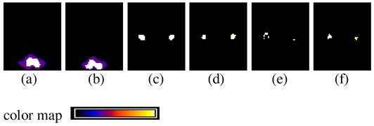
We presented these 48 activation maps, and corresponding values for F, as input to fGAMMA. fGAMMA detected three clusters, shown in Figure 7. Cluster 1 (Figure 7(b)) corresponds to the strongly activated voxels in the visual region (A). Clusters 2 and 3 (Figure 7(d)) are within the motor region (B); fGAMMA detected two clusters in region B because there does not exist a single activation pattern in region B, as there does in region A. As shown in Figure 8, R₂ and R₃ jointly covers all activation patterns in region B for all subjects. Setting pa(F) to RV₁, RV₂, and RV₃ clearly differentiates the two groups.

Figure 7.

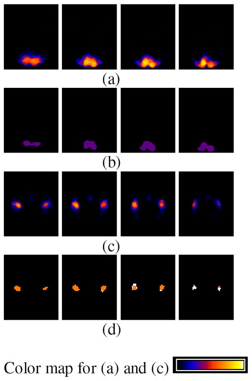
The summation of activation maps for all subjects and the label field Λ^mode for the simulated data. The summation map shows the probability of voxel activation in the activation maps. (a) summation map in region A; slice numbers from left to right are 14, 16, 18, 20, respectively. (b) cluster 1 (purple) in Λ^mode. (c) summation map in region B; slice numbers from left to right are 35, 37, 39, 41, respectively. (d) cluster 2 (yellow) and 3 (white) in Λ^mode.

Figure 8.

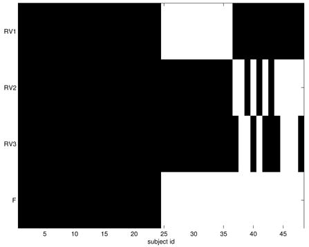
Representative voxels and F for the simulated-data experiment. For representative voxels, black is 0 (not activated) and white is 1 (activated). For F, black is 1 (control) and white is 2 (exposed to stimulus).

Model-aggregation results are shown in Figures 9 and 10. The empirical model distribution arising from jackknife sampling, , is shown in Figure 9. Let denote the BN generated using all subjects without resampling (i.e., D). In Figure 9, we also show how many BNs in model ensemble are identical to , and annotate that portion of the histogram with . fGAMMA generated 11 different BN patterns in the model ensemble; the mode has frequency 0.79; is identical to in this simulated data set. Therefore, we conclude that is stable under data perturbation. Class maps are shown in Figure 10; there are differences among {Λ^k | = }. The label field Λ^mode is consistent with the majority of Λ^k

Figure 9.

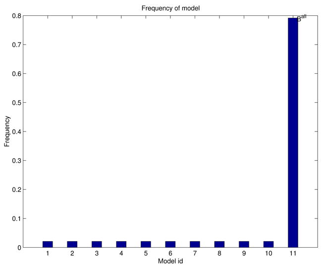
Model-frequency histogram for the simulated-data experiment.

Figure 10.

Class maps for the simulated-data experiment. (a) , slice 16; (b) , slice 20; (c) , slice 37; (c) , slice 39; (e) , slice 39; (f) , slice 41.

To demonstrate that fGAMMA can detect multivariate associations among brain regions and F that cannot be identified by GLM-based mass-univariate methods, we performed a two-sample t-test on the same simulated data. In particular, we used the contrast map of the visual area in the Voxbo data set as the contrast map for region A, and that of the motor areas in the Voxbo data set as the contrast map for region B. We then computed t statistics for these contrast maps to compare between group voxel-activation differences. The resulting t-map is depicted in Figure 11; both regions A and B demonstrate more activation foci in group 2 than in group 1. The t-test does detect a region within which activation levels are significantly different across groups; however, these results cannot be used to delineate interactions among regions and F. Although the activation patterns of these two regions are quite different during the task, we cannot distinguish them based on only this t-map.

Figure 11.

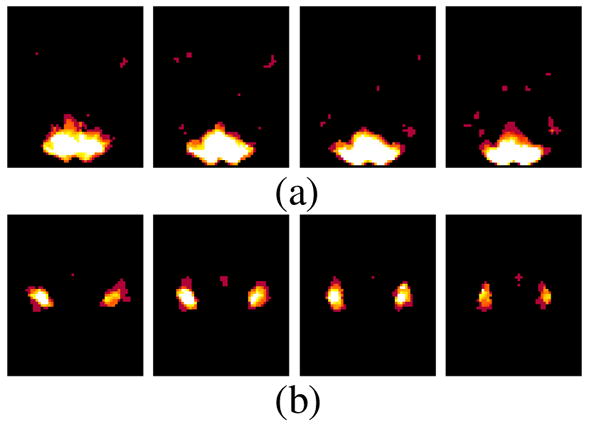
The t-map for comparing voxel-activations across groups for the simulated data. Brighter color represents higher t-statistic value.(a) t-map in region A; slice numbers from left to right are 14, 16, 18, 20, respectively. (b) t-map in region B; slice numbers from left to right are 35, 37, 39, 41, respectively.

3.2 A study of young, nondemented, and demented older adults

In addition to testing fGAMMA on simulated data, we applied fGAMMA to data from a previously published fMR study of nondemented young adults, nondemented older adults, and demented older adults (Buckner et al. (2000)). A subject with dementia of the Alzheimer type manifests cognitive deficits such as memory impairment, language disturbance, or impaired ability to carry out motor activities despite intact motor function. We obtained data for 41 subjects from the registry of the Washington University Alzheimer Disease Research Center (Buckner et al. (2000)). Participants were English-speaking and right-handed. People with neurological, psychiatric, or medical illness that could cause dementia were excluded from this study. Older subjects were assessed with the Clinical Dementia Rating (CDR) (Morris (1993)), where CDR=0 indicates no dementia, CDR=0.5 indicates very mild dementia, and CDR=1 indicates mild dementia of the Alzheimer type. There were 14 participants (5 male) with mean age 21.1 years in the young-adult group. The nondemented older-adult group consisted 14 subjects (5 male) with CDR=0, with mean age of 74.9 years. The demented older-adult group consisted of 13 participants (6 male), with a mean age of 77.2 years; 8 of them had CDR=0.5 and 5 had CDR=1. Functional-MR images were acquired with an asymmetric spin-echo sequence sensitive to BOLD contrast (TR=2.68 sec, T2* evolution time = 50 msec). Image resolution was 3.75 × 3.75 × 8 mm³. These data are publicly available from the National fMR Data Center (http://www.fmridc.org), with access number 2-2000-1118w.

There were two trial conditions in this experiment. In condition 1, a 1.5-second duration visual stimulus was presented. The visual stimulus was an 8-Hz counter-phase flickering checkerboard. Each subject was instructed to press a key with his/her right index finger at stimulus onset. In condition 2, a pair of visual stimuli with interval 5.36 seconds were presented. Each subject underwent 4 runs of 15 trials; 8 image volumes were collected during each trial. Conditions 1 and 2 were pseudo-randomly intermixed; in each run, eight of the trials were of one condition, and the other seven were of the other condition.

We used SPM2 to detect activated voxels for condition 1 (the isolated visual stimulus). We applied a p-value threshold of 0.005 to the t-map, with a multiple-comparison correction based on Gaussian random-field theory (Worsley et al. (1992)). We chose this p-value to control the false-positive rate; although it resulted in low statistical power, we can be confident in activation foci that survive this threshold.

As expected, all three groups showed activation in motor cortex on the left, and in visual cortex. We applied fGAMMA to detect activation-map differences among (I) young vs. nondemented older, (II) young vs. demented older, and (III) nondemented older vs. demented older subjects. In these three analyses, F = 2 indicated young, young, and nondemented-older groups, respectively. The aggregated label fields, and model frequencies are shown in Figure 12, and Figure 13.

Figure 12.

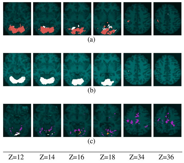
Aggregated label fields are overlaid on transverse sections for each study. The aggregated label fields are superimposed on the average anatomic image in the MNI coordinate system. For (a) and (b), the anatomic image is from a young subject. For (c), it is from a nondemented older subject. (a) Study I: young vs. nondemented older; cluster 1 (RV₁) is red; cluster 2 (RV₂) is white. (b) Study II: young vs. demented older; cluster 1 (RV₁) is white. (c) Study III: nondemented older vs. demented older; cluster 1 (RV₁) is purple; cluster 2 (RV₂) is yellow; cluster 3 (RV₃) is white.

Figure 13.

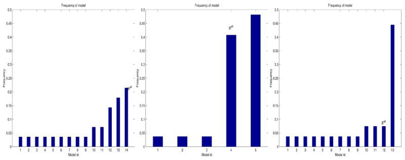
Model-frequency histograms for experiment 2. From left to right: young vs. nondemented older; young vs. demented older; nondemented older vs. demented older.

The CPTs for F are shown in Table 1. Each row in a CPT, denoted by θ_ij, represents a conditional distribution of F given a parent state. We introduce a measure f_RV to describe the relative frequency of the occurrence of a parent state. Combining the CPT for F and f_RV, we can determine the strongest co-occurrence patterns of RV and F, and use them to understand the underlying cognitive processes. In this manner, in Table 1, for study I, we can infer that F has a probabilistic AND type association with RV₁ and RV₂. A dominant co-occurrence pattern was [RV₁ = 0, RV₂ = 0, F = 1], which means if there is no activation in RV₁ or RV₂, that subject will have a high probability (0.94) of being a nondemented-older subject. We observed this pattern with frequency P (RV₁ = 0, RV₂ = 0, F = 1) = P (F = 1 | RV₁ = 0, RV₂ = 0)P (RV₁ = 0, RV₂ = 0) = 0.94 × 0.50 = 0.47. In study II, the association among RV₁ and F was linear. If RV₁ was activated, we could predict this subject was a young adult with high probability (0.88). For study III, the association among RV₁, RV₂, RV₃, and F was complicated. The strongest co-occurrence pattern was [RV₁ = 0, RV₂ = 0, RV₃ = 0, F = 1], suggesting that the demented older group had less activation. Other strong co-occurrence patterns were [RV₁ = 1, RV₂ = 0, RV₃ = 0, F = 2] and [RV₁ = 0, RV₂ = 1, RV₃ = 1, F = 2]; these two co-occurrence patterns characterized the non-demented older group; that is, the non-demented older group tended to have activation in RV₁ only, or in RV₂ and RV₃.

Table 1.

Conditional probability tables for F, and parent-state frequencies (f_RV). Top: young vs. nondemented older; middle: young vs. demented older; bottom: nondemented older vs. demented older. Values in brackets are posterior variance to characterize uncertainty in estimation.

RV1	RV2	P (F = 1 | RV1, RV2)	P (F = 2 | RV1, RV2)	fRV
0	0	0.94 (0.003)	0.06 (0.003)	0.50
1	0	0.10 (0.008)	0.90 (0.008)	0.28
0	1	0.25 (0.038)	0.75 (0.038)	0.07
1	1	0.17 (0.020)	0.83 (0.020)	0.14
RV1	P (F= 1 | RV1)	P (F = 2 | RV1)	fRV
0	0.93 (0.004)	0.07 (0.004)	0.44
1	0.12 (0.006)	0.88 (0.006)	0.55
RV1	RV2	RV3	P (F = 1 | RV1, RV2, RV3)	P (F = 2 | RV1, RV2, RV3)	fRV
0	0	0	0.92 (0.006)	0.08 (0.006)	0.37
1	0	0	0.14 (0.015)	0.86 (0.015)	0.18
0	1	0	0.50 (0.036)	0.50 (0.036)	0.15
1	1	0	0.33 (0.056)	0.67 (0.056)	0.04
0	0	1	0.50 (0.050)	0.50 (0.050)	0.07
1	0	1	0.50 (0.083)	0.50 (0.083)	0.00
0	1	1	0.17 (0.020)	0.83 (0.020)	0.15
1	1	1	0.33 (0.056)	0.67 (0.056)	0.04

The label fields for analyses I and II clearly show reduced spatial extents of activation for nondemented and demented older subjects, compared to young subjects; these results are consistent with those reported in the original analysis of these data (Buckner et al. (2000)). The regions manifesting group differences are primarily in the visual areas. The results of study II are more stable than those of study I: for study II contained 5 BN patterns, whereas for study I contained 14 patterns, and the frequency of the mode was lower in study I than in study II. In addition, the label field from study II was more spatially compact than that from study II, suggesting that the demented older/young difference was greater than the nondemented older/young difference. The label field from study III was noisy; the noise in the label field results from noise in the activations of both the nondemented older and demented older subjects. As expected, fGAMMA’s ability to detect a valid pattern characterizing group differences decreased with increasing noise.

We could not detect a difference among groups for motor-area activation in studies I and II. Similarly, D’Esposito et al. reported that the hemodynamic-response amplitudes of voxels in activated motor areas were similar for young and old adults (D’Esposito et al. (1999)). Buckner et al. reported similar response amplitudes of voxels in activated motor areas across young, nondemented older, and demented older subjects (Buckner et al. (2000)). Our findings are consistent with those previously reported in the literature, and suggest that there is no difference in the spatial extents of motor-area activation between young and old adults.

Figure 13 demonstrates that model aggregation leads to greater stability of models generated by fGAMMA. In studies II and III, is different from .

4 Discussion and Conclusions

We have described a method for group analysis of fMR data; our approach uses a Bayesian-network representation to identify linear or nonlinear multivariate probabilistic associations among groups of activated voxels and a clinical variable F. In addition, fGAMMA incorporates data resampling to select a model that is robust under data perturbation.

fGAMMA and GLM-based approaches, such as random-effects analysis, attempt to detect activation-pattern differences among experimental groups. Both approaches share the same general two-stage analytic framework: within-subject analysis to detect individual activation, followed by between-subject analysis to detect group differences. The major differences between fGAMMA and GLM-based approaches are threefold. First, fGAMMA treats group membership as a categorical variable and generates a model to represent associations among regions and that variable; regions critical to detecting group differences constitute the Markov blanket of the group variable in the Bayesian network generated by fGAMMA. In contrast, GLM-based approaches directly compare the voxel-wise activation differences across groups. Second, fGAMMA is a multivariate nonparametric method, whereas GLM-based approaches, as typically applied to fMR analysis, are mass-univariate and assume normality. Third, fGAMMA adopts a model-selection approach to find an optimal model of the fMR data, as measured by maximization of a fitness function. In contrast, GLM-based approaches compute voxelwise parametric statistics, with multiple-comparison correction.

Empirically, GLM-based approaches cannot handle the case of functional degeneracy, or complex nonlinear associations among regions and the group-membership variable, whereas fGAMMA was designed to handle these scenarios. The simulated functional-degeneracy study in Section 3.1 clearly demonstrates this difference. Our method focuses on the detection of associations among voxels (or voxel groups) and F, whereas most mass-univariate methods, such as random-effects analysis, are formulated to detect region-specific effects.

Various types of structure-function associations can also be detected by other group-analysis methods. For example, linear structure-function associations among regions and F can be revealed by a t-test, and the AND relationship can be obtained using a conjunction analysis with conjunction null (Nichols et al. (2005)).

There exist many multivariate methods for group analysis, such as (Coulon et al. (2000); Calhoun et al. (2001); Svensen et al. (2002); Esposito et al. (2005)). These methods have different strengths and assumptions. For example, independent component analysis for group inference, proposed in Calhoun et al. (2001), reveals spatiotemporal modes of signal variability. This method imposes a common space of observations for all sources, although the activation time courses of different subjects may differ. We plan to apply these multivariate methods to a test data set that contains interesting structure-function associations, such as functional degeneracy, and compare them with fGAMMA.

We assume that the activation pattern associated with the underlying neural process is consistent across subjects, and dominates the data. Although lack of statistical power or noise could affect CPT values, the number of representative voxels, and the spatial shape and extent of ROIs, the types of structure-function associations detected tend not to change because of BN’s ability to encode uncertainty. Equation (3) may help distinguish results due to high noise or small sample size from inherently high variability. We plan to extend our work towards comprehensive evaluation of fGAMMA, including noise level, the choice of threshold, and the number of subjects, among other parameters.

In constructing a Bayesian network to model associations among regions and F, fGAMMA detects regions that, when considered together, are strongly associated with group differences. In this respect, our Bayesian-network approach is fundamentally different from classification methods, such as support vector machines (Cox and Savoy (2003); Mitchell et al. (2004); Zhang et al. (2005)). fGAMMA does not maximize a metric of classification accuracy; rather, fGAMMA maximizes modeling of the joint probability distribution that characterize structure-function associations in the fMR data. To extend fGAMMA to support classification, we are developing a classification algorithm that uses voxels in a label field as features.

Our simulations demonstrated that fGAMMA can identify nonlinear multivariate associations among voxels and F. The results of our analysis of studies involving young, nondemented older, and demented older subjects are consistent with those reported in the literature, demonstrating the validity of our approach. However, we plan additional validation experiments with simulated and with previously analyzed data.

Our current implementation requires binary voxel and clinical variables, which may lead to loss of information. In the fMR study of young, nonde-mented, and demented older adults, we found our results were consistent with those found by applying standard statistical methods to the same data without discretization. These results suggest that discretization, as applied in fGAMMA, does not cause severe loss of information.

fGAMMA currently can analyze only one clinical or group-membership variable. We plan to extend fGAMMA to handle more than one clinical variable. We expect that after this extension of our work, fGAMMA will be able to show how several clinical variables, such as age and sex, as well as group membership, jointly modulate interactions among region activations.

One problem with fGAMMA is the computational cost of model aggregation, which requires running the model-generation algorithm many times. In a fMR study involving dozens of subjects with approximately 10⁶ voxels, with spatial resolution 3 × 3 × 3 mm³, we can obtain results in several hours using a readily available desktop workstation. In a study involving more subjects and voxels, a parallel version of fGAMMA may be required to produce results in a timely manner.

Appendix

We describe the procedure of belief-map generation in this section. The goal of belief-map generation is to infer the equivalence set E based on the similarity map S.

Provided that the number of clusters c is known, the prior for L is a MRF such that

$$P(\mathbf{L})=\frac{1}{Z}{e}^{-{\sum }_i{\sum }_{j:j\in mb(i)}\beta {(\mu (i)-\mu (j))}^2},$$ (10)

where μ(i) denotes the centroid of the cluster to which voxel i belongs, and β is a parameter controlling global smoothness. Let ϒ = {μ₁; μ_2;,…, μ_c} where μ_i is the centroid of cluster i. ϒ and β are the hyperparameters of L. In this MRF model, if L_i and L_j are in clusters a and b, respectively, and the centroids of clusters a and b are close to each other, the probability of observing this pattern is greater than that in the case in which the centroids of clusters a and b are far from each other.

The goal is to find L̂ and ϒ̂ such that

$$\{\widehat{\mathbf{L}},\widehat{\mathrm{\Upsilon }}\}=\underset{\mathbf{L},\mathrm{\Upsilon }}{\text{argmax}}P(\mathbf{L},\mathrm{\Upsilon }\mid \mathbf{S}).$$ (11)

L̂ and ϒ̂ are the MAP estimation of L and ϒ, given S. We use a generalized expectation-maximization (EM) method to solve this problem. The generalized EM algorithm iteratively searches for L and ϒ. In iteration k, the algorithm first searches for L̂(k) such that L̂(k) = argmax_L P (L | S, ϒ̂ (k − 1)), and then finds ϒ̂(k) that maximizes P (ϒ | S, L̂(k)). Finding ϒ̂(k) is straightforward: given L̂(k), for all voxels in cluster i, the empirical mean of their intensities in the similarity map is the estimator of μ_i. The key issue is how to compute L̂(k).

From Bayes’ theorem, P (L | S, ϒ) ∝ P (S | L, ϒ)P (L | ϒ). Assume that

$$P(\mathbf{S}\mid \mathbf{L},\mathrm{\Upsilon })\propto e^{-{\sum }_{i}U(L_i,S_i)},$$ (12)

where U(L_i, S_i) is a function that describes the relationship between the similarity map and the label field. For this purpose, we use U(L_i, S_i) = (S_i − μ(i))²; thus, we assume that S_i = μ(i) + N_i, where N_i represents independently and identically distributed Gaussian white noise. Let ψ (L_i, L_j) = e^{−β(μ(i) − μ(j))2} and φ(L_i, S_i) = e^{−(S_i− μ(i))2}. From Bayes’ theorem and Equations (10) and (12), we have

$$P(\mathbf{L}\mid \mathbf{S},\mathrm{\Upsilon })=\frac{1}{Z}\prod _{i,j}\psi (L_i,L_j)\prod _i\phi (L_i,S_i),$$ (13)

where Z is a normalization constant. Therefore, the goal is to find the MAP estimate of L based on equation (13). That is,

$$\widehat{\mathbf{L}}=\underset{\mathbf{L}}{\text{argmax}}\prod _{i,j}\psi (L_i,L_j)\prod _i\phi (L_i,S_i).$$ (14)

To solve this optimization problem, we use loopy belief propagation (LBP). The LBP algorithm works in an iterative fashion. On each iteration, the message m_ij (L_j) contains the information that is propagated from node i to node j regarding relative likelihoods for particular states that j might assume. If L_i has r states, then m_ij (L_j) is a vector of length r. On each iteration, each node L_i sends a message m_ij (L_j) to nodes in its Markov blanket mb(L_i). The updating rule for m_ij (L_j) is as follows:

$$m_{ij}(L_j)\leftarrow \sum _{L_i}\phi (L_i,S_i)\psi (L_i,L_j)\prod _{k\in mb(i)\backslash j}{m}_{ki}(L_i).$$ (15)

The belief for node i is a vector of length r; it represents the marginal probability distribution for this node, and is determined by the product of the evidence term φ (L_i, S_i) and the messages coming into node i:

$$b(L_i)=\frac{1}{Z_i}\phi (L_i,S_i)\prod _{j\in mb(i)}{m}_{ji}(L_i),$$ (16)

where Z_i is a normalization constant. LBP updates m_ij and b(L_i), based on equations (15) and (16). On each iteration, each node computes the messages for all nodes in its Markov blanket. Once all messages are calculated, the messages are delivered to their recipient nodes; these messages are then used to update the messages and beliefs on the next iteration. If |b_k(L_i) − b_k−1(L_i)| ≈ 0 for any i, then LBP converges, and the hidden label of L_i is set to be the mode of belief vector b(L_i).

The number of clusters is estimated based on GVRC metric (Chen and Herskovits (2005a)). Based on the experimental results in (Chen and Herskovits (2005a)), belief-map generation is not very sensitive to the global smoothness parameter β.

References

- Breiman L. Bagging predictors. Machine Learning. 1996;24 (2):123–140. [Google Scholar]
- Breiman L. Random forests. Machine Learning. 2001;45 (1):5–32. [Google Scholar]
- Buckner RL, Snyder AZ, Sanders AL, Raichle ME, Morris JC. Functional brain imaging of young, nondemented, and demented older adults. Journal of Cognitive Neuroscience Supplement. 2000;12 (2):24–34. doi: 10.1162/089892900564046. [DOI] [PubMed] [Google Scholar]
- Calhoun VD, Adali T, Pearlson GD, Pekar JJ. A method for making group inferences from functional MRI data using independent component analysis. Human Brain Mapping. 2001;14 (3):140–151. doi: 10.1002/hbm.1048. [DOI] [PMC free article] [PubMed] [Google Scholar]
- Chen R, Herskovits EH. KDD ’05: Proceeding of the eleventh ACM SIGKDD international conference on Knowledge discovery in data mining. ACM Press; New York, NY, USA: 2005a. A Bayesian network classifier with inverse tree structure for voxelwise magnetic resonance image analysis; pp. 4–12. [Google Scholar]
- Chen R, Herskovits EH. Graphical-model based morphometric analysis. IEEE Transaction on Medical Imaging. 2005b;24 (10):1237–1248. doi: 10.1109/TMI.2005.854305. [DOI] [PubMed] [Google Scholar]
- Chen Y, Fu S, Iversen SD, Smith SM, Matthews PM. Testing for dual brain processing routes in reading: a direct contrast of Chi-nese character and pinyin reading using fMRI. Journal of Cognitive Neuro-sciencei. 2002 October;14 (7):1088–1098. doi: 10.1162/089892902320474535. [DOI] [PubMed] [Google Scholar]
- Cooper GF, Herskovits EH. A Bayesian method for the induction of probabilistic networks from data. Machine Learning. 1992;9:309–347. [Google Scholar]
- Coulon O, Mangin JF, Poline JB, Zilbovicius M, Roumenov D, Sam-son Y, Frouin V, Bloch I. Structural group analysis of functional activation maps. NeuroImage. 2000;11 (6):767–782. doi: 10.1006/nimg.2000.0580. [DOI] [PubMed] [Google Scholar]
- Cox DD, Savoy RL. Functional magnetic resonance imaging (fMRI) “brain reading”: detecting and classifying distributed patterns of fMRI activity in human visual cortex. NeuroImage. 2003;19:261–270. doi: 10.1016/s1053-8119(03)00049-1. [DOI] [PubMed] [Google Scholar]
- D’Esposito M, Zarahn E, Aguirre GK, Rypma B. The effect of normal aging on the coupling of neural activity to the bold hemodynamic response. NeuroImage. 1999 July;10 (1):6–14. doi: 10.1006/nimg.1999.0444. [DOI] [PubMed] [Google Scholar]
- Edelman GM, Gally JA. Degeneracy and complexity in biological systems. Proceedings of the National Academy of Sciences. 2001;98:13763–13768. doi: 10.1073/pnas.231499798. [DOI] [PMC free article] [PubMed] [Google Scholar]
- Esposito F, Scarabino T, Hyvarinen A, Himberg J, Formisano E, Co-mani S, Tedeschi G, Goebel R, Seifritz E, Salle FD. Independent component analysis of fMRI group studies by self-organizing clustering. NeuroImage. 2005;25 (1):193–205. doi: 10.1016/j.neuroimage.2004.10.042. [DOI] [PubMed] [Google Scholar]
- Freund Y, Schapire RE. International Conference on Machine Learning. 1996. Experiments with a new boosting algorithm; pp. 148–156. [Google Scholar]
- Friston KJ. Functional and effective connectivity in neuroimaging: a synthesis. Human Brain Mapping. 1994;2:56–78. [Google Scholar]
- Friston KJ, Holmes AP, Worsley KJ, Poline JP, Frith CD, Frack-owiak RSJ. Statistical parametric maps in functional imaging: a general linear approach. Human Brain Mapping. 1995;2:189–210. [Google Scholar]
- Gelman A, Carlin JB, Stern HS, Rubin DB. Bayesian Data Analysis. Chapman Hall/CRC; Boca Raton: 1995. [Google Scholar]
- Heckerman D, Geiger D, Chickering DM. Learning Bayesian networks: The combination of knowledge and statistical data. Machine Learning. 1995;20:197–243. [Google Scholar]
- Herskovits EH. Computer-based probabilistic-network construction. Ph.D. thesis, Stanford University; 1991. [Google Scholar]
- Koller D, Sahami M. Towards optimal feature selection. Proceedings of the 13th International Conference on Machine Learning (ML); 1996. pp. 284–292. [Google Scholar]
- Lazar NA, Luna B, Sweeney JA, Eddy WF. Combining brains: a survey of methods for statistical pooling of information. NeuroImage. 2002 June;16 (2):538–550. doi: 10.1006/nimg.2002.1107. [DOI] [PubMed] [Google Scholar]
- Mitchell TM, Hutchinson R, Niculescu RS, Pereira F, Wang X, Just M, Newman S. Learning to decode cognitive states from brain images. Machine Learning. 2004 October;57 (12):145–175. [Google Scholar]
- Morris JC. The Clinical Dementia Rating (CDR): current version and scoring rules. Neurology. 1993;43 (11):2412–2414. doi: 10.1212/wnl.43.11.2412-a. [DOI] [PubMed] [Google Scholar]
- Nichols T, Brett M, Andersson J, Wager T, Poline JB. Valid conjunction inference with the minimum statistic. NeuroImage. 2005;25 (3):653–660. doi: 10.1016/j.neuroimage.2004.12.005. [DOI] [PubMed] [Google Scholar]
- Noppeney U, Penny WD, Price CJ, Flandin G, Friston KJ. Identification of degenerate neuronal systems based on intersubject variability. NeuroImage. 2006;30 (3):885–890. doi: 10.1016/j.neuroimage.2005.10.010. [DOI] [PubMed] [Google Scholar]
- Pearl J. Probabilistic Reasoning in Intelligent Systems. Morgan Kauf-mann; 1988. [Google Scholar]
- Penny WD, Holmes AP, Friston KJ. Human Brain Function. 2. Academic Press; 2003. Random effects analysis. [Google Scholar]
- Phillips JA, Humphreys GW, Noppeney U, Price CJ. The neural substrates of action retrieval: An examination of semantic and visual routes to action. Visual Cognition. 2002;9 (4):662–684. [Google Scholar]
- Price CJ, Friston KJ. Degeneracy and cognitive anatomy. Trends in Cognitive Sciences. 2002;6 (10):416–421. doi: 10.1016/s1364-6613(02)01976-9. [DOI] [PubMed] [Google Scholar]
- Svensen M, Kruggel F, Benali H. ICA of fMRI group study data. NeuroImage. 2002;16:551–563. doi: 10.1006/nimg.2002.1122. [DOI] [PubMed] [Google Scholar]
- Tamm L, Menon V, Johnston CK, Hessl DR, Reiss AL. fMRI study of cognitive interference processing in females with fragile X syndrome. Journal of Cognitive Neurosciencei. 2002 February;14 (2):160–171. doi: 10.1162/089892902317236812. [DOI] [PubMed] [Google Scholar]
- Weiss Y. Interpreting images by propagating Bayesian beliefs. In: Mozer M, Jordan M, Petsche T, editors. Advances in Neural Information Processing Systems. Vol. 9. 1997. pp. 908–915. [Google Scholar]
- Worsley KJ, Liao CH, Aston J, Petre V, Duncan GH, Morales F, Evans AC. A general statistical analysis for fMRI data. NeuroImage. 2002 January;15 (1):1–15. doi: 10.1006/nimg.2001.0933. [DOI] [PubMed] [Google Scholar]
- Worsley KJ, Marrett S, Neelin P, Evans AC. A three-dimensional statistical analysis for CBF activation studies in human brain. Journal of Cerebral Blood Flow and Metabolism. 1992;12:900–918. doi: 10.1038/jcbfm.1992.127. [DOI] [PubMed] [Google Scholar]
- Yedidia JS, Freeman WT, Weiss Y. Understanding belief propagation and its generalizations. Morgan Kaufmann Publishers; Ch: 2003. Exploring Artificial Intelligence in the New Millennium; pp. 239–270. [Google Scholar]
- Zhang L, Samaras D, Tomasi D, Volkow N, Goldstein R. Proceedings of the IEEE International Conference on Computer Vision and Pattern Recognition. 2005. Machine learning for clinical diagnosis from functional magnetic resonance imaging; pp. 1211–1217. [Google Scholar]