Accommodating Linkage Disequilibrium in Genetic-Association Analyses via Ridge Regression

Abstract

Large-scale genetic-association studies that take advantage of an extremely dense set of genetic markers have begun to produce very compelling statistical associations between multiple makers exhibiting strong linkage disequilibrium (LD) in a single genomic region and a phenotype of interest. However, the ultimate biological or “functional” significance of these multiple associations has been difficult to discern. In fact, the LD relationships between not only the markers found to be associated with the phenotype but also potential functionally or causally relevant genetic variations that reside near those markers have been exploited in such studies. Unfortunately, LD, especially strong LD, between variations at neighboring loci can make it difficult to distinguish the functionally relevant variations from nonfunctional variations. Although there are (rare) situations in which it is impossible to determine the independent phenotypic effects of variations in LD, there are strategies for accommodating LD between variations at different loci, and they can be used to tease out their independent effects on a phenotype. These strategies make it possible to differentiate potentially causative from noncausative variations. We describe one such approach involving ridge regression. We showcase the method by using both simulated and real data. Our results suggest that ridge regression and related techniques have the potential to distinguish causative from noncausative variations in association studies.

Introduction

The availability of cost-efficient genotyping technologies and the development of very dense maps of polymorphic loci within the human genome have paved the way for large-scale genetic-association studies. These studies, which include comprehensive whole-genome association (WGA) studies, exploit linkage disequilibrium (LD) relationships between variations at marker loci genotyped on a large number of subjects and variations at loci that reside in the vicinity of these marker loci.^1,2 Many of these studies have produced findings that are very compelling from a statistical point of view and have generated test statistics quantifying the association strength between multiple loci within particular genomic regions and specific phenotypes with p values as small as 10⁻⁸ or 10⁻¹².^1,2 As compelling as these statistical associations are, however, the fact that multiple markers within single genomic regions that are in strong LD—and hence highly correlated—are associated with a particular phenotype makes it difficult to separate in these regions the individual variations that are likely to be causally associated to the phenotype of interest from those that are simply in LD with causal loci.

This phenomenon and problem are not particularly new to genetic analysis because the inability to resolve the precise location of an offending mutation has plagued traditional pedigree and sibling-pair-based linkage studies, as well as genealogically informed haplotype studies, for years as a result of the limited number of recombination events that can be exploited in such studies.^3–5 Although the use of (predominantly) unrelated individuals and the smaller intermarker distances for which strong LD is observed in general population-based case-control association studies is thought to help overcome this problem, recent studies suggest that this problem still, albeit within the smaller genomic regions suggested by these studies, is an area of concern. The following three recent examples are cases in point (although there are many others): Easton et al.⁶ identified multiple single-nucleotide polymorphisms (SNPs) exhibiting strong association with breast cancer (MIM 114480) in the FGFR2 (MIM 176943) and TNRC9 (MIM 611416) gene regions and used standard logistic-regression-analysis procedures to find the most strongly associated SNPs with breast cancer among the many that showed association with breast cancer in these regions; Gudmundson et al.⁷ identified on chromosome 17 multiple SNPs that appeared to be significantly associated with prostate cancer (MIM 176807) and also used multiple logistic regression to resolve the putative “functionally” or “causally” associated variants; and Haiman et al.⁸ identified on chromosome 8q24 seven SNPs that appeared to exhibit independent associations with prostate cancer after use of logistic regression to resolve their contributions to prostate cancer risk among other SNPs that exhibited strong to moderate LD in the same region with these seven.

The use of multiple regression-like analysis methods in contexts in which multiple loci are taken as independent (or predictor) variables with a phenotypic measure taken as a dependent variable would be appropriate only if the variations at those loci are not in strong LD. Thus, traditional regression-analysis models and procedures are highly problematic when strong LD exists among the variations of interest that will be taken as independent variables. For example, it may be the case that there are multiple, functionally relevant loci that are within a particular genomic region and that happen to have alleles that are in LD. In this case, standard regression analyses that do not account for the multicollinearity (i.e., LD) among the predictor SNP variables can produce misleading results.⁹ In addition, it is known that in instances for which there is moderate-to-strong multicollinearity among predictor variables, standard regression analyses break down because of singularities in matrices requiring inversion involved in relevant computations (although this can be remedied in some instances with some numerical tricks).⁹ Thus, although regression methods can be useful and appropriate tools for modeling relationships between genetic variations and phenotypes of interest, they must be used with caution in situations in which a researcher is interested in identifying the most likely functionally or causally relevant SNPs among a number of SNPs that exhibit moderate to strong LD.

We propose the use of ridge-regression procedures for accommodating correlations (i.e., LD) between genetic variations in association studies. Ridge regression was introduced by Hoerl and Kennard¹⁰ in 1970 and has been recently used in a number of settings for large-scale data analysis, such as marker-assisted selection,¹¹ expression-array analysis,¹² and haplotype-association analysis.¹³ As discussed in the Material and Methods and Discussion sections, ridge regression offers many advantages over the traditional multiple-regression models and standard least-squares-regression-coefficient estimation procedures. For example, ridge regression can deal with a number of predictor variables that far exceeds the number of subjects and can also deal with situations in which the predictors are highly correlated. Thus, ridge regression has potential in genetic-association-analyses settings involving multiple variations in LD with each other for which the goal is to differentiate functional from nonfunctional SNPs. Other methodologies have been proposed for this purpose and include conditional haplotype analysis,¹⁴ conditional logistic regression,¹⁵ and Hoh's set-association method.¹⁶ However, these methods do not allow one to simultaneously quantify the effect of each SNP individually along with the combined effect of the SNPs in a way that accommodates the LD between the SNPs.

We first describe the mechanics behind ridge regression and how ridge regression can be used to account for correlated predictor variables such as multiple SNPs in strong LD; some subset of these SNPs are causally associated with an independent variable (i.e., phenotype) of interest. We showcase the utility of the ridge-regression method by using previously published data involving the CHI3L2 gene (MIM 601526). We also compare the results produced by ridge regression to those obtained with traditional multiple-regression methods via simulation studies. Finally, we consider limitations of the proposed ridge-regression approach as well as areas for further research.

Material and Methods

The Multiple-Linear-Regression Model

Let X be an n × p matrix where p is the number of SNPs (or other forms of genetic variation) genotyped on a set of n individuals, and Y be an n-dimensional vector containing phenotype values for each individual. SNP genotypes can be coded as dummy variables with homozygotes being assigned a 0.0, heterozygotes being a 0.5, and opposite homozygotes being a 1.0 under an additive model or, for models involving dominance or recessive effects, with heterozygotes being assigned a 0.0 or 1.0, respectively. For the analyses we describe below, we assumed an additive model. Under the usual linear-regression model: Y = Xβ + ɛ, we can obtain estimates of the regression coefficients β by minimizing the residual sum of squares:

$$\mathit{RSS}=(Y-X\beta )\text{'}(Y-X\beta )$$ (1)

such that the vector of regression coefficients is estimated by:

$${\widehat{\beta }}^{\mathit{MLR}}=\text{arg min}\left(\mathit{RSS}\right)={(X\text{'}X)}^{-1}X\text{'}Y$$ (2)

The solution to Equation 2 either can not be obtained or is highly problematic if (1) p > > n or if (2) some variables are moderately to strongly correlated, because in this situation, the (X'X) matrix could be singular and therefore not invertible. In this case, one must select a subset of variables that are not as strongly correlated for use in the model. Although it has been suggested in the literature that a selection of “target” SNPs for ultimate analysis in regression contexts can be pursued via, e.g., clustering methods, principal-component analysis, or forward stepwise selection, this strategy is not ideal because if many SNPs are correlated and one is chosen for use in an analysis on the basis of its correlation with others, the chosen SNP may not actually be the functional SNP. In addition, it could be the case that there exist more than one functional SNP among those that are correlated, such that choosing one to represent a cluster of correlated SNPs would not reflect the fact that more than one position in the sequence is phenotypically relevant. In addition, Frank and Friedman¹⁷ have shown that ridge regression is preferable to principal-component and subset-selection methods in many contexts. Also, the “local” optima found by stepwise-regression approaches to predictor variable selection may not represent the true “global” optimum¹⁸ because of the potentially large number of predictor variables (SNPs) that might be considered. Finally, many methods such as principal-component and cluster-analysis methods lack ease of result interpretation and power because each SNP is not tested separately or associated or provided with a metric—such as regression coefficient—whose statistical significance can be gauged. In contrast, ridge regression allows direct analysis of all variables (i.e., SNPs or genetic variations) in the model and, in addition, quantifies the individual effects of each of several correlated SNPs, which, as has been pointed out, is crucial in WGA studies if one is to ultimately identify the most likely causally associated SNPs with a phenotype.

The Ridge-Regression Model

As an alternative to choosing a subset of SNPs as potential phenotype predictors that are meant to represent the effects of variations in a particular genomic region, ridge regression has the advantage of including all SNPs in the model and both providing regression coefficients that can be tested for significance for each SNP individually and accommodating potential linkage disequilibrium among them. Ridge regression has been around since the 1970s as a statistical tool used to deal with multicollinearity and to avoid problems related to small sample size and/or a large number of predictor variables.^19,20 Ridge regression can be viewed as a special case of “regularized” regression because it puts constraints on the size of the coefficients to control large variances associated with resulting estimates. In brief, ridge regression works by “shrinking” the effect of redundant variables (e.g., SNPs in strong LD) to zero by imposing a penalty on the size of their coefficients:

$${\widehat{\beta }}^{\mathit{Ridge}}={(X\text{'}X+kI)}^{-1}X\text{'}Y$$ (3)

where the ridge parameter k > 0 represents the degree of shrinkage. By adding the term kI, the ridge-regression model reduces multicollinearity and prevents the matrix X′X from being singular even if X itself is not of full rank. Note that if k = 0, the ridge-regression coefficients are equal to those from the traditional multiple-regression model. Ridge regression does not allow any one regression coefficient to get very large, so it protects against overfitting and usual high variances associated with correlated coefficients. Although there is a great deal in the literature on methods of estimating the value of k, such as generalized cross-validation,²¹ all of them are data driven. Finding the optimal method of choosing k is beyond the goal of this paper. In this paper, we used the original definition of k provided by Hoerl, Kennard, and Baldwin;²² it is easy to implement, and, as shown later, performs well.

To test the significance of each coefficient estimated from ridge regression, one can compute a Wald-test, i.e., dividing the coefficient estimate by its standard error, which is defined as the square-root of his variance:

$$\mathit{VAR}\left(\widehat{\beta }\right)=(W^{-1}X\text{'})(W^{-1}X\text{'})\text{'}$$ (4)

$$\text{where}W=(X\text{'}X+\mathit{kI}).$$

Here, the test statistic follows a Student t distribution as in traditional least-squares-regression-model-based tests of regression coefficients.²³ However, the number of degrees of freedom used for inference is assumed to be the number of “effective degrees of freedom,” and this is smaller than the number of free parameters in the model. The efficient number of degrees of freedom is defined by:

$$\mathit{EDF}=\mathit{trace}(X{(X\text{'}X+\mathit{kI})}^{-1}X\text{'})=\mathit{trace}({(X\text{'}X+\mathit{kI})}^{-1}X\text{'}X)$$ (5)

and it equals the rank of X when k = 0. Consequently, the tests are equivalent to those from a traditional multiple-regression model if there is no correlation among independent variables; i.e., if the variables are independent. Note that independent variables could be centered or standardized prior to the regression analysis, but the literature is not clear about how such standardization would improve performance. We find that the use of standardized variables can give problematic results, so we have not used standardization in our analyses.

The CEPH Family Gene Expression Data as an Example Data Set

We applied three analysis methods to SNPs within the CHI3L2 gene and CHI3L2 gene expression as a phenotype²⁴ in order to compare their performance: single-locus analysis (i.e., standard regression analysis with a single SNP as a predictor), a standard multiple-linear-regression model, and a ridge-regression model. We obtained SNP data collected on 57 unrelated CEPH individuals from the International HapMap Project database. These individuals were chosen by International HapMap Project researchers for massive, genome-wide genotyping studies²⁵ and were also later used for assessment of gene expression patterns obtained from immortalized lymphocytes collected on the HapMap subjects.²⁶ We downloaded the gene expression via GEO accession number GSE2552. Our analyses excluded the individual labeled NA06993 in the gene expression studies because detailed analysis of HapMap data suggested that the sample associated with this person is likely to have derived from an unreported relative. We also added data associated with the individual labeled NA12056 because gene expression data for this individual are now available. We ultimately downloaded phased, haplotype data that were on the 22 autosomal chromosomes from the HapMap (phase 1) database and that were available on the 57 CEPH individuals. We eliminated monomorphic SNPs from our analyses. Missing genotypes for particular individuals were filled in by imputing genotypes with a combination of available parental genotype data, the most likely combination of genotypes observed in the regions with the missing genotype data, and standard haplotype-inference analyses.²⁷ We used the average of the of log₂-transformed gene expression levels associated with each subject for the phenotype.

Because true functional SNPs in the CHI3L2 gene are unknown, we also simulated continuous phenotypes by generating a varying number (1–25) of equally distributed “functional” SNPs among the 26 SNPs of the CHI3L2 region. Phenotypes were generated according to a standard normal distribution based on the genotypic information at the hypothetical functional loci. To create associations between the phenotype and CHI3L2 SNPs for each person, we increased the corresponding phenotype by 2 standard deviations (SDs) each time that a particular allele was observed at a “functional” locus. A total of 1000 sets of phenotypes were generated in this manner. For each of the 25 different cases with a fixed number of “functional” SNPs, we applied the single-locus analysis and the ridge-regression method to a 1000 sets of simulated phenotypes. In these simulations, we did not consider traditional multiple regression because the high degree of correlation among the SNPs in the CHI3L2 generated enormous numerical difficulties in fitting the model (emphasizing its nonutility as a general method for identifying functional SNPs from a group of SNPs in LD). Rather than using an arbitrary p value or significance threshold and method to correct for multiple testing, we used ROC curves to assess the sensitivity and specificity of the methods in differentiating functional from nonfunctional loci. Instead of displaying the results for each of the 25 different settings (i.e., the 25 different assumptions about the number of functional loci), we averaged the ROC curves over the simulated data sets and settings, assuming the various number of functional loci as described below.

Simulation Study

Our simulation study was divided in two parts. First, we sought to compare the performance of three regression methods (single-locus regression, traditional multiple linear regression, and ridge regression) in settings involving multiple SNPs in LD for which only some subset are causally associated with a continuous phenotype. Second, we investigated the effect of the LD strength between two SNP loci on the performance of each regression method for differentiating the causal association between one of the SNPs and the phenotype from the SNP in LD with that causal SNP. All the calculations and analyses were programmed and implemented in R version 2.4.1 and Python version 2.3.5. For the first simulation studies that did not involve the CHI3L2 gene, we assumed sample sizes of either 100 or 500. We also considered a genomic region with 20 biallelic loci within it, with the number of functional loci influencing a continuous phenotype ranging from 1–19, with the allele-specific effect size at the functional loci equal to either 0.5 or 1.0 phenotypic SD units. We generated linkage disequilibrium among the loci by fixing the frequency of the different haplotypes that could be constructed from the 20 loci. Thus, if many haplotypes are assumed to have a frequency of 0.0, this would create strong LD between the loci. We assumed all simulated loci had two alleles, coded as 0 and 1. For each person, two genotypes were randomly generated by random sampling from the subset of haplotypes according to their frequencies.

It should be understood that generating multiple (i.e., >3) SNP loci with fixed prior-specified LD strengths between and allele frequencies on the basis of a simple analytic formula is not trivial. In addition, there are an infinite number of possible situations that we could have explored in terms of allele frequencies and LD strengths. We chose to concentrate on situations for which there was moderate to strong LD among the loci as quantified by the D' measure of LD. We ultimately simulated SNP data by assuming that 14 of the 2²⁰ possible haplotypes had frequencies >0.0 with individual frequencies of 0.32, 0.24, 0.33, and 0.01 for the 11 remaining haplotypes. Use of these frequencies creates strong (D' > 0.55; but highly variable, over all the simulations) LD among each pair of loci and varying allele frequencies, as described in the Results section.

Phenotypes were generated according to a standard normal distribution. To create associations between the phenotype and the simulated SNPs, we increased individual phenotypes by a value equal to an assumed “effect size” for each “1” allele an individual has at a functional locus. In this setting, all, functional loci were assumed to have effect of equal size. We generated 100 data sets for each combination of the assumed number of subjects, number of functional loci, and effect-size parameter. We ensured that each functional locus did, in fact, have an effect in each simulate data set by rejecting simulated data sets in which the locus was monomorphic.

Ultimately, each of the three regression methods was applied to each simulated data set. Thus, for the single-locus analyses and the ridge-regression analyses, we obtained 100 p values for each of the 20 loci corresponding to the significance level of a test involving the relevant regression coefficient. However, for the multiple-regression method, only the SNPs that could enter in the model without causing a singularity were considered. Consequently, the results of our simulations are biased toward more favorable results for traditional multiple regression. Because the power of any one technique may come at the expense of higher type I (α) error, we chose to compare sensitivity (power, i.e., 1-probability of a type II error) at a common specificity (i.e., 1-α, or 1-probability of a type I error). Otherwise, the sensitivity of one method could be artificially higher than that of another because of its larger α level. Because we were unable to choose an appropriate a priori threshold t that would result in a certain type I error over all the analysis methods compared, we employed receiver operating characteristic (ROC) curves to control for different α levels. Because results correspond to p values, we varied the threshold t from 0 to 1 in steps of 0.0001 for a total of 1000 data points for each ROC curve.

Because the “true” number of functional loci in any realistic association analysis is usually unknown a priori, we averaged the ROC curves over the results obtained over the simulated data sets containing various number of functional loci. For illustration of how this was done, consider p values obtained from the simulated data sets by applying one specific method (e.g., ridge regression) to each of the 100 replicates × 19 data sets with varying number of functional loci, for a small effect size (0.5) and 100 people. For the first value of t, we calculated sensitivity and specificity. Sensitivity is the proportion of the 19,000 p values corresponding to the [(1 + 2 + 3 + … + 19) × 100] functional loci that are smaller than t. Similarly, specificity is the proportion of the remaining 19,000 p values corresponding to the [(19 + 18 + 17 + … + 1) × 100] nonfunctional loci that are greater than t. We recalculated sensitivity and specificity for each value of t and obtained ROC curves by plotting “sensitivity” against “1-specificity.”

For the second simulation study, we again compared the three analysis methods: single-locus regression analysis, standard multiple regression analysis, and ridge regression. We set the sample size to 100 subjects, the number of loci to two, and the number of functional loci to one with an effect size of 0.5. Here, we constrained our attention to the most difficult case for detecting an association, i.e., situations involving a small effect size and a small sample size, in order to more easily distinguish the performance of each method because it is easier for any method to detect associations when only one locus is functional. Instead of choosing a number of different haplotypes with fixed frequency, allele frequencies at the two loci were randomly assigned according to a uniform distribution. We generated 1,000,000 simulated data sets. For each set of simulations, we recorded the theoretical and the empirical LD between the two loci as well as the allele frequencies, and for each method, the p value obtained from test statistics measuring the association between the loci and the simulated phenotype. The results were stratified for different values of D' and different allele frequencies, and again ROC analyses were used. For each D' and allele frequency stratum, and for each of the 1000 threshold values of t, sensitivity was calculated as the proportion of significant p values corresponding to the functional locus, and specificity was calculated as the proportion of nonsignificant p values corresponding to the nonfunctional locus.

Results

Ridge Regression Applied to the CHI3L2 Region

We considered the association analysis of SNPs in the CHI3L2 gene region and CHI3L3 gene expression as a phenotype as originally discussed by Cheung et al.²⁶ and, more recently, Wessel, Libiger, and Schork.²⁴ We applied each of the three aforementioned regression methods to the 26 SNPs within the CHI3L2 region. Figure 1 displays the linkage disequilibrium between the loci and shows that the majority of the pairs of SNPs are in strong linkage disequilibrium. Thus, it is not surprising that the results of the use of traditional multiple linear regression suffered from the multicolinearity problems and could fit only 11 of the 26 SNPs in a same model, thereby resulting in several missing coefficient values and no significant p value (Table 1). Here, the choice of the SNPs that have entered the model was based on the algorithm implemented in the R software (version 2.4.1). Note that the application of a forward stepwise procedure in which SNPs are entered into a model in sequence in which the SNPs with the strongest effect enter first, the SNP with the second strongest effect given the effect of the first enters second, etc. In this case, only three SNPs (rs755467, rs2274232, and rs2251715) entered the model; thus, the majority of the SNPs are not tested despite the fact that they might ultimately be causal and functional and in LD with a SNP that entered into the model.

Figure 1.

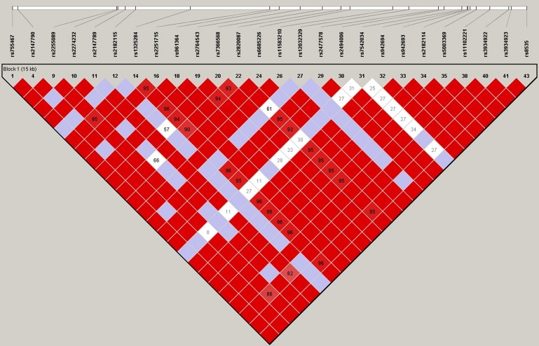
Haploview Plot of 26 SNPs in the CHI3L2 Gene

Haploview (versions 3.32) plot of the pairwise linkage disequilibrium among the 26 loci within the CHI3L2 gene region as obtained from the International HapMap Project database.

Table 1.

Regression Analysis Results for SNPs within the CHI3L2 Gene from the HapMap Gene Expression Data

SNP ID	Single Locus Analysis			Multiple Regression			Ridge Regression
	Estimate	SD	Pr (>|t|)	Estimate	SD	Pr (>|t|)	Estimate	SD	P (>|t|)
Intercept	9.06	0.16	7.01E−51∗	8.90	2.37	0.0005	2.61	0.34	1.20E−09∗
rs755467	1.01	0.18	8.74E−07∗	0.92	1.35	0.5002	1.11	0.31	8.32E−04∗
rs2147790	−0.07	0.25	7.90E−01	0.36	0.49	0.4709	0.34	0.54	5.28E−01
rs2255089	−0.47	0.19	1.37E−02	0.15	1.38	0.9139	1.43	0.43	1.80E−03∗
rs2274232	0.39	0.27	1.62E−01	0.62	0.61	0.3171	0.85	0.16	2.66E−06∗
rs2147789	−0.38	0.17	3.30E−02	−0.05	0.39	0.9026	−0.01	0.44	9.84E−01
rs2182115	−0.51	0.28	6.75E−02	−0.26	0.38	0.4981	−0.24	0.42	5.80E−01
rs1325284	−0.86	0.19	3.97E−05∗	−1.89	1.18	0.1183	−0.09	0.14	5.04E−01
rs2251715	−0.47	0.19	1.44E−02	NA	NA	NA	0.75	0.19	2.21E−04∗
rs961364	0.99	0.18	1.62E−06∗	0.23	0.59	0.6949	0.28	0.64	6.58E−01
rs2764543	−0.86	0.19	3.97E−05∗	NA	NA	NA	−0.09	0.14	5.04E−01
rs7366568	−0.69	0.25	6.79E−03	0.72	0.46	0.1262	0.69	0.51	1.86E−01
rs2820087	−0.76	0.20	4.54E−04∗	−0.23	0.44	0.602	−0.22	0.49	6.53E−01
rs6685226	−0.10	0.26	7.06E−01	−0.44	0.58	0.4472	−0.40	0.62	5.22E−01
rs11583210	−0.37	0.21	9.11E−02	0.23	1.27	0.8598	0.65	0.96	5.01E−01
rs12032329	0.39	0.27	1.62E−01	NA	NA	NA	0.85	0.16	2.66E−06∗
rs2477578	−0.86	0.19	3.97E−05∗	NA	NA	NA	−0.09	0.14	5.04E−01
rs2494006	−0.74	0.20	3.90E−04∗	0.30	0.53	0.5760	0.26	0.59	6.59E−01
rs7542034	0.07	0.81	9.29E−01	0.21	0.84	0.8038	0.42	0.76	5.82E−01
rs942694	−0.78	0.19	1.47E−04∗	0.88	0.84	0.3014	0.78	0.86	3.68E−01
rs942693	−0.86	0.19	3.97E−05∗	NA	NA	NA	−0.09	0.14	5.04E−01
rs2182114	−0.86	0.19	3.97E−05∗	NA	NA	NA	−0.09	0.14	5.04E−01
rs5003369	−0.86	0.19	3.97E−05∗	NA	NA	NA	−0.09	0.14	5.04E−01
rs11102221	−0.34	0.21	1.15E−01	NA	NA	NA	2.68	0.75	9.12E−04∗
rs3934922	0.94	0.18	3.11E−06∗	NA	NA	NA	1.79	0.35	6.76E−06∗
rs3934923	−0.86	0.19	3.97E−05∗	NA	NA	NA	−0.09	0.14	5.04−01
rs8535	1.01	0.18	8.74E−07∗	NA	NA	NA	1.11	0.31	8.32E−04∗

The asterisks represent significant p values (<1.92E−03) at an overall 5% level with a Bonferroni correction. “NA” stands for not applicable (the multiple-regression procedure could not fit the model with this SNP because of multicollinearity).

On the basis of a conservative Bonferroni correction, the single-locus analysis and the ridge regression, which allowed testing of all 26 SNPs individually, 14 and eight SNPs were significant, respectively, at an overall 5% level. Among those, 11 and five SNPs were significant in one method and not the other. Because the real effect of each SNP (i.e., whether it is functional or not) is unknown in this data set, we cannot tell whether this observed difference is due to higher type 1 error or lower power, for one of the two methods, thus motivating our simulation study. What we can say is that accounting for the LD among the SNPs radically changed which of the SNPs is likely to be causally associated with the CHI3L2 phenotype on the basis of statistical analysis. Also, we want to emphasize the fact that the results from the ridge regression depend on the choice of the method used to estimate the ridge parameter k. Figure 2 shows the ridge trace for the 26 coefficient estimates for varying values of k (x axis). One could conceivably use this type of graph to decide on the appropriate value of k.^10,19 We used the Hoerl, Kennard, and Baldwin²² method for generating the value for k, which produced a k = 0.1215, a full model with R² = 0.61, and an error sum of square of 26.93. However, we tried the ridge regression on the same data set with varying values of k, and for each analysis, the set of significant SNPs (i.e., ridge-regression coefficient p < 0.0019) were the same (data not shown). The most important elements of Table 1 and Figure 2 concern not only the change in the values of the coefficients, as well as their significance levels, but also the change of sign for some of the coefficients. This suggests that by not accommodating LD in relevant association-analysis models, one might be mistaken with respect to the actual effect of the alleles on a phenotype.

Figure 2.

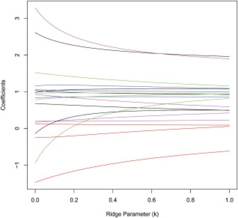
The Ridge Trace Associated with Analysis of the CHI3L2 SNPs

Each curve corresponds to the ridge regression coefficient estimate for one of the 26 loci of the CHI3L2 region for varying value of the ridge parameter k (x axis).

We also pursued simulations that took advantage of the real genotypes obtained on the 57 subjects, but used simulated phenotypes whose associations with particular SNPs were determined a priori, and applied the single-locus analysis and the ridge-regression methods to the resulting data sets. Because we knew the “true” functional loci, we were able to estimate sensitivity and specificity of each method to identify those loci. Figure 3 demonstrates the higher performance of the ridge-regression method in comparison to the single-locus analysis. As mentioned in the Material and Methods section, ROC curves were averaged among the varying number of functional loci. For the different combinations of sample size and effect size, ridge regression always performed best. As expected, the single-locus analysis is unable to differentiate causal SNPs from those merely correlated (i.e., in LD with) those causal SNPs.

Figure 3.

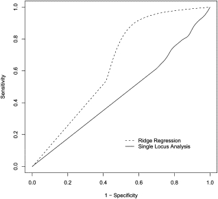
ROC Curves Comparing the Performance of the Single-Locus Analysis and the Ridge-Regression Methods

Each ROC curve represents the performance of one of the two regression methods when trying to detect association between the 26 SNPs of the CHI3L2 region and a simulated phenotype (solid line = single-locus regression; dashed line = ridge regression). Results are averaged among varying number (1–25) of functional loci.

Simulation Study

Figure 4 depicts the theoretical LD strength between the loci used to generate SNPs for the first component of our simulation studies. The pairwise D' values range from 0.57 to 1.0 with an arithmetic average of 0.85. Figure 5 provides the average ROC curves over the simulations obtained for each of the three analysis methods in differentiating causal from noncausal SNPs. Figure 5 clearly shows that ridge regression performs best when trying to differentiate causal from noncausal associations between moderate to highly correlated SNPs and a continuous phenotype. As mentioned in the Material and Methods section, ROC curves were averaged over the various assumed number of functional loci. For the different combinations of sample size and effect size, ridge regression always performed best. As expected, single-locus analysis is unable to differentiate causal SNPs from those merely correlated (i.e., in LD) with causal SNPs.

Figure 4.

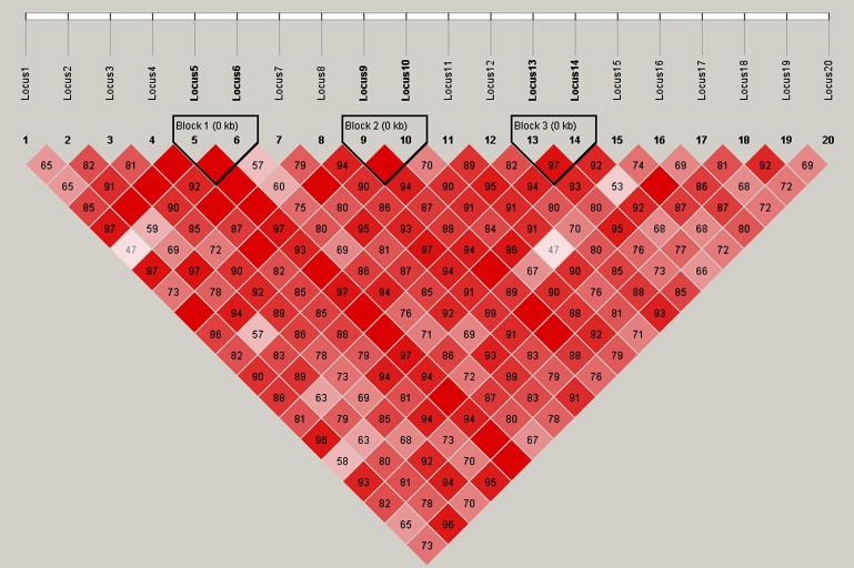
Haploview Plot of 20 SNPs Used in the Simulation Studies

Haploview (version 3.32) plot of the theoretical pairwise linkage disequilibrium among the 20 loci calculated from the respective frequencies of the 14 haplotypes used in simulating the genotype data for the first component of our simulation studies. Dashed line indicates ridge regression, dotted line indicates multiple linear regression, and solid line indicates single-locus analysis.

Figure 5.

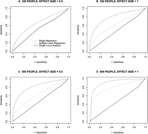
ROC-Curve-Based Overall Comparison of Analysis Methods

Each ROC curve represents the performance of one of the three regression methods when trying to detect association between a set of 20 loci and a phenotype (solid line = single-locus regression; dotted line = standard multiple regression; dashed line = ridge regression). Results are averaged among varying number (1–19) of functional loci. Dashed line indicates ridge regression, dotted line indicates multiple linear regression, and solid line indicates single-locus analysis.

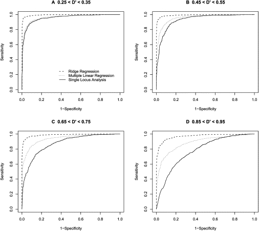
For the second component of our simulation studies, in which two loci of varying LD strength were generated, one of which was causally related to a trait, all the methods performed reasonably well when there was little LD between the SNP alleles, as expected, although ridge regression performed best (Figures 6–8). We stratified the simulations according to the frequency of the first locus as well as the LD strength between the two loci and then averaged the results to generate ROC curves. Figures 6, 7, and 8 show results for the first locus allele frequencies of 0.25, 0.50, and 0.75, respectively. In all cases, ridge regression performed better in differentiating the causal locus from the noncausal locus merely in LD with the causal locus. Single-locus analysis is, as expected, the method most affected by increasing LD strength in differentiating causal from noncausal loci.

Figure 6.

ROC-Curve-Based Comparison of Analysis Methods Based on an Allele Frequency of 0.25

ROC curves comparing the performance of three regression-based methods for association analysis when the frequency of the “1” allele is 0.25. Each ROC curve represents the performance of one of the three regression methods when trying to detect association between a 2 loci (one functional and one nonfunctional) and a phenotype (solid line = single-locus regression; dotted line = standard multiple regression; dashed line = ridge regression). The sample size was fixed to 100 people, and the functional loci had an effect of size 0.5. Dashed line indicates ridge regression, dotted line indicates multiple linear regression, and solid line indicates single-locus analysis.

Figure 7.

ROC-Curve-Based Comparison of Analysis Methods Based on an Allele Frequency of 0.50

ROC curves comparing the performance of three regression-based methods for association analysis when the frequency of the “1” allele is 0.50. Each ROC curve represents the performance of one of the three regression methods when trying to detect association between a 2 loci (one functional and one nonfunctional) and a phenotype (solid line = single-locus regression; dotted line = standard multiple regression; dashed line = ridge regression). The sample size was fixed to 100 people, and the functional loci had an effect of size 0.5. Dashed line indicates ridge regression, dotted line indicates multiple linear regression, and solid line indicates single-locus analysis.

Figure 8.

ROC-Curve-Based Comparison of Analysis Methods Based on an Allele Frequency of 0.75

ROC curves comparing the performance of three regression-based methods for association analysis when the frequency of the ‘1’ allele is 0.75. Each ROC curve represents the performance of one of the three regression methods when trying to detect association between a 2 loci (one functional and one non-functional) and a phenotype (solid line = single locus regression; dotted line = standard multiple regression; dashed line = ridge regression). The sample size was fixed to 100 people, and the functional loci had an effect of size 0.5.

Discussion

Studies seeking to identify genetic variations that are likely to influence common complex diseases via genetic-association analysis will continue to grow as the cost of genotyping technologies are reduced. However, ultimately differentiating “causal” variations from those variations merely in LD with causal variations is not trivial in genetic-association-study contexts, especially when extremely dense panels or maps of markers are used, because the LD between the variations at those loci is likely to be strong. Although laboratory assays can be used for assessing the likely functional significance of particular variations—and hence provide insight into the potential causal nature of the associations involving certain SNPs—these assays can be costly and time consuming, thereby making statistical methods for prioritizing variations for consideration in such laboratory assays even more valuable.

It should also be noted that virtually all of the recently published GWA studies made use of single-locus-based analyses. Single-locus-based analyses, as shown by our simulation studies, may lack the statistical sophistication to resolve causal or functional from noncausal or nonfunctional loci as well as to detect multiple-locus effects within a genomic region, and this can lead both false-positive and false-negative results. Many researchers have, in fact, taken advantage of two-stage designs²⁸ to minimize false-positive results. However, two-stage designs are expensive and time consuming because they require a second population and retesting variations that, ultimately, may not be truly associated with the phenotype of interest. In addition, because the actual number of false positives one can expect in an association study is unknown a priori, it may be the case that several causal SNPs will go undetected in an initial study and hence not be investigated in a follow-up study. Ultimately, then, analyzing (or even reanalyzing) WGA data with a more powerful statistical tool such as the ridge regression should increase the chance of finding compelling associations that can be considered in additional studies.

We have shown that ridge regression outperforms standard multiple regression and traditional single-locus-based analyses in the identification of variations that are functionally or causally related to a trait from those that are merely in LD with those causal variants. Despite this, there are a number of issues and possible ridge-regression extensions that should be considered. First and foremost is the issue of the choice of the ridge parameter, k. Although there are many strategies for choosing an optimal value for k, there is no consensus on the best or most general way to choose k. In addition, it is possible to implement models for which different values of k for each potential predictor or independent (i.e., SNP) variable are used, although the properties of such generalized ridge-regression procedures have not been explored in full.²⁹ We find that adding virtually any positive value of k in Equation 3 makes a difference on the regression estimates. Obviously, more work in this area is needed. In addition, we concentrated on situations in which the phenotype of interest is continuous in nature, but the ridge-regression approach can be applied in case-control or dichotomous phenotype situations through the use of ridge logistic regression.³⁰ Despite these and other even more obvious issues (such as assumptions of normality and linearity in the gene-phenotype relationship), the advantages of accommodating LD in differentiating the most likely causal variations from those that are merely correlated or in LD with the causal variations, the ability to analyze many variations in a single model, computational efficiency, and ease of interpretation of results clearly suggest ridge regression could be great value to researchers pursuing dense-map, large-scale genetic-association studies.

As mentioned previously, one possible use of the proposed ridge-regression procedure involves its application in the basic analysis stages of WGA studies. Although it may be theoretically possible to consider all SNPs simultaneously in a single analysis, we don't recommend this and rather believe that one could exploit a “moving-window” approach in which sets of adjacent SNPs are analyzed for association simultaneously (unpublished data). Thus, for example, one could consider a moving-window-based strategy in which some number, l, of adjacent loci are used in the analysis in order to test for associations between variations at those l loci and the phenotype of interest. After this analysis is performed, the window is moved one locus away, and the analysis is repeated. This is continued until the entire genome is covered. Leveraging the independent effects of multiple causal variations in a single genomic region could increase the evidence that variations in that region are associated with the phenotype of interest over single-locus analyses. The choice of the window size is obviously arbitrary but can be varied so that locus effects that appear to work in aggregate or in isolation could be identified, thus allowing for flexibility in the analysis. Because several loci are tested in these situations, one should consider the use of a multiple testing correction such as false discovery rate. In the event that genome regions are identified that appear to have variations within them that are associated with a particular phenotype, one could analyze all the variations across all these loci in a single model. Interaction and covariate terms could also be incorporated because of the flexibility of the regression model.

Other methods for accommodating correlations among predictor variables in regression-analysis-like contexts have been proposed. For example, partial least-squares analysis attempts to find variables that have high variance and high correlation with particular independent variable;²⁰ the “LASSO”-based regression technique, which exploits “penalties” for terms that do not have predictive power in the model relative to others could also be used,²⁰ and generalized estimating equations (or GEEs) models treat correlations between variables as nuisance parameters to focus attention on the ultimate relationships between a set of sets of variables. A comparison of the power and utility of these various methods with ridge regression in the context of genetic-association studies involving variations in LD would be of great value because our results suggest that ridge regression provides a simple, flexible, and reliable method for differentiating the most likely set of causal variations from those variations that are merely in LD with those causal variations.

Web Resources

The URLs for data presented herein are as follows:

• Gene Expression Omnibus, http://www.ncbi.nlm.nih.gov/geo/

• HapMap, www.hapmap.org

• Online Mendelian Inheritance in Man (OMIM), http://www.ncbi.nlm.nih.gov/Omim/

• RidgeReg (available in the near future), http://polymorphism.scripps.edu

References

- 1.Couzin J., Kaiser J. Genome-wide association. Closing the net on common disease genes. Science. 2007;316:820–822. doi: 10.1126/science.316.5826.820. [DOI] [PubMed] [Google Scholar]
- 2.Topol E.J., Murray S.S., Frazer K.A. The genomics gold rush. JAMA. 2007;298:218–221. doi: 10.1001/jama.298.2.218. [DOI] [PubMed] [Google Scholar]
- 3.Ott J. The Johns Hopkins University Press; Baltimore: 1991. Analysis of Human Genetic Linkage. [Google Scholar]
- 4.Kruglyak L., Lander E.S. High-resolution genetic mapping of complex traits. Am. J. Hum. Genet. 1995;56:1212–1223. [PMC free article] [PubMed] [Google Scholar]
- 5.Houwen R.H., Baharloo S., Blankenship K., Raeymaekers P., Juyn J., Sandkuijl L.A., Freimer N.B. Genome screening by searching for shared segments: mapping a gene for benign recurrent intrahepatic cholestasis. Nat. Genet. 1994;8:380–386. doi: 10.1038/ng1294-380. [DOI] [PubMed] [Google Scholar]
- 6.Easton D.F., Pooley K.A., Dunning A.M., Pharoah P.D., Thompson D., Ballinger D.G., Struewing J.P., Morrison J., Field H., Luben R. Genome-wide association study identifies novel breast cancer susceptibility loci. Nature. 2007;447:1087–1093. doi: 10.1038/nature05887. [DOI] [PMC free article] [PubMed] [Google Scholar]
- 7.Gudmundsson J., Sulem P., Steinthorsdottir V., Bergthorsson J.T., Thorleifsson G., Manolescu A., Rafnar T., Gudbjartsson D., Agnarsson B.A., Baker A. Genome-wide association study identifies a second prostate cancer susceptibility variant at 8q24. Nat. Genet. 2007;39:631–637. doi: 10.1038/ng1999. [DOI] [PubMed] [Google Scholar]
- 8.Haiman C.A., Patterson N., Freedman M.L., Myers S.R., Pike M.C., Waliszewska A., Neubauer J., Tandon A., Schirmer C., McDonald G.J. Multiple regions within 8q24 independently affect risk for prostate cancer. Nat. Genet. 2007;39:638–644. doi: 10.1038/ng2015. [DOI] [PMC free article] [PubMed] [Google Scholar]
- 9.Draper N.R., Smith H. Second Edition. John Wiley and Sons; New York: 1981. Applied Regression Analysis. [Google Scholar]
- 10.Hoerl A.E., Kennard R.W. Ridge regression: Biased estimation for nonorthogonal problems. Technometrics. 1970;12:55–67. [Google Scholar]
- 11.Whittaker J., Thompson R., Denham M.C. Marker-assisted selection using ridge regression. Genet. Res. 2000;75:249–252. doi: 10.1017/s0016672399004462. [DOI] [PubMed] [Google Scholar]
- 12.Hastie T., Tibshirani R. Efficient quadratic regularization for expression arrays. Biostatistics. 2004;5:329–340. doi: 10.1093/biostatistics/5.3.329. [DOI] [PubMed] [Google Scholar]
- 13.Li Y., Sung W.K., Liu J.J. Association mapping via regularized regression analysis of single-nucleotide-polymorphism haplotypes in variable-sized sliding windows. Am. J. Hum. Genet. 2007;80:705–715. doi: 10.1086/513205. [DOI] [PMC free article] [PubMed] [Google Scholar]
- 14.Valdes A.M., Erlich H.A., Noble J.A. Human leukocyte antigen class I B and C loci contribute to Type 1 Diabetes (T1D) susceptibility and age at T1D onset. Hum. Immunol. 2005;66:301–313. doi: 10.1016/j.humimm.2004.12.001. [DOI] [PMC free article] [PubMed] [Google Scholar]
- 15.Zavattari P., Lampis R., Motzo C., Loddo M., Mulargia A., Whalen M., Maioli M., Angius E., Todd J.A., Cucca F. Conditional linkage disequilibrium analysis of a complex disease superlocus, IDDM1 in the HLA region, reveals the presence of independent modifying gene effects influencing the type 1 diabetes risk encoded by the major HLA-DQB1, -DRB1 disease loci. Hum. Mol. Genet. 2001;10:881–889. doi: 10.1093/hmg/10.8.881. [DOI] [PubMed] [Google Scholar]
- 16.Hoh J., Wille A., Ott J. Trimming, weighting, and grouping SNPs in human case-control association studies. Genome Res. 2001;11:2115–2119. doi: 10.1101/gr.204001. [DOI] [PMC free article] [PubMed] [Google Scholar]
- 17.Frank I., Friedman J. A statistical view of some chemometrics regression tools (with discussion) Technometrics. 1993;35:109–148. [Google Scholar]
- 18.Zhang B., Horvath S. Finding the best ridge regression subset by genetic algorithms: applications to multi-locus quantitative trait mapping. Conf. Proc. IEEE Eng. Med. Biol. Soc. 2004;4:2793–2796. doi: 10.1109/IEMBS.2004.1403798. [DOI] [PubMed] [Google Scholar]
- 19.Gruber M.H.J. Marcel Dekker, Inc.; New York: 1998. Improving Efficiency by Shrinkage: The James-Stein and Ridge Regression Estimators. [Google Scholar]
- 20.Hastie T., Tibshirani R., Friedman J. Springer; New York: 2001. The Elements of Statistical Learning: Data Mining, Inference, and Prediction. [Google Scholar]
- 21.Golub G.H., Heath M., Wahba G. Generalized cross-validation as a method for choosing a good ridge parameter. Technometrics. 1979;21:215–223. [Google Scholar]
- 22.Hoerl A.E., Kennard R.W., Baldwin K.F. Ridge regression: Some simulations. Comm. Statist. Theory Methods. 1975;4:105–123. [Google Scholar]
- 23.Halawa A.M., El Bassiouni M.Y. Tests of regression coefficients under ridge regression models. J. Statist. Comput. Simulation. 2000;65:341–356. [Google Scholar]
- 24.Wessel J., Schork N.J. Generalized genomic distance-based regression methodology for multilocus association analysis. Am. J. Hum. Genet. 2006;79:792–806. doi: 10.1086/508346. [DOI] [PMC free article] [PubMed] [Google Scholar]
- 25.Altshuler D., Brooks L.D., Chakravarti A., Collins F.S., Daly M.J., Donnelly P. A haplotype map of the human genome. Nature. 2005;437:1299–1320. doi: 10.1038/nature04226. [DOI] [PMC free article] [PubMed] [Google Scholar]
- 26.Cheung V.G., Spielman R.S., Ewens K.G., Weber T.M., Morley M., Burdick J.T. Mapping determinants of human gene expression by regional and genome-wide association. Nature. 2005;437:1365–1369. doi: 10.1038/nature04244. [DOI] [PMC free article] [PubMed] [Google Scholar]
- 27.Salem R.M., Wessel J., Schork N.J. A comprehensive literature review of haplotyping software and methods for use with unrelated individuals. Hum. Genomics. 2005;2:39–66. doi: 10.1186/1479-7364-2-1-39. [DOI] [PMC free article] [PubMed] [Google Scholar]
- 28.Wang H., Thomas D.C., Pe'er I., Stram D.O. Optimal two-stage genotyping designs for genome-wide association scans. Genet. Epidemiol. 2006;30:356–368. doi: 10.1002/gepi.20150. [DOI] [PubMed] [Google Scholar]
- 29.Walker S.G., Page C.J. Generalized ridge regression and a generalization of the Cp statistic. J. Appl. Stat. 2001;28:911–922. [Google Scholar]
- 30.Le Cressie S., van Houwelingen J. Ridge estimators in logistic regression. Appl. Stat. 1992;41:191–201. [Google Scholar]