An Approximate Bayesian Computation Approach to Overcome Biases That Arise When Using Amplified Fragment Length Polymorphism Markers to Study Population Structure

Abstract

There is great interest in using amplified fragment length polymorphism (AFLP) markers because they are inexpensive and easy to produce. It is, therefore, possible to generate a large number of markers that have a wide coverage of species genomes. Several statistical methods have been proposed to study the genetic structure using AFLPs but they assume Hardy–Weinberg equilibrium and do not estimate the inbreeding coefficient, F_IS. A Bayesian method has been proposed by Holsinger and colleagues that relaxes these simplifying assumptions but we have identified two sources of bias that can influence estimates based on these markers: (i) the use of a uniform prior on ancestral allele frequencies and (ii) the ascertainment bias of AFLP markers. We present a new Bayesian method that avoids these biases by using an implementation based on the approximate Bayesian computation (ABC) algorithm. This new method estimates population-specific F_IS and F_ST values and offers users the possibility of taking into account the criteria for selecting the markers that are used in the analyses. The software is available at our web site (http://www-leca.ujf-grenoble.fr/logiciels.htm). Finally, we provide advice on how to avoid the effects of ascertainment bias.

THE range of many if not most species is spatially subdivided and can be generally described as a metapopulation composed of many local populations. Thus, the genetic diversity of a species is spatially structured into within and between components. This so-called genetic structure has important implications for the evolution of species and knowledge of it is fundamental for applications in the domains of conservation biology and genetic epidemiology. Genetic structuring is typically assessed using the so-called F-statistics first introduced by Wright (1951), who distinguished three statistics, F_IS, F_ST, and F_IT. They have been widely used in population genetics but the interpretation of results has been difficult because of ambiguities about their definitions. Loosely speaking, F_IS represents the shared ancestry between alleles of an individual relative to the population and is usually called the inbreeding coefficient. F_ST represents the shared ancestry within the population relative to the metapopulation and is usually used to measure the degree of differentiation among populations. Finally, F_IT represents the shared ancestry between alleles of an individual relative to the metapopulation and provides an overall measure of inbreeding. Traditionally the study of population genetic structuring is done using a global F_ST coefficient, which ignores differences in the strength of genetic drift across populations. Over a decade ago, Balding and Nichols (1995) proposed the use of population specific F_ST's in the context of a migration–drift equilibrium model. More recently, Balding (2003) proposed a general framework to rigorously define all F-statistics using the beta–binomial model proposed by Balding and Nichols (1995). This new formulation, and in particular its multiallelic version, the multinomial Dirichlet, has been used recently to address many different problems. Ciofi et al. (1999) used it to distinguish between two types of model of population structure and to estimate population-specific F_ST coefficients, Falush et al. (2003) used it for clustering individuals into populations, Beaumont and Balding (2004) used it to identify candidate loci under natural selection, and Foll and Gaggiotti (2006) used it to identify biotic/abiotic factors that are responsible for the observed spatial structuring of genetic diversity and to infer population history.

There are a wide variety of molecular markers available for studying genetic structure. The use of codominant markers such as allozymes, microsatellites, or SNPs leads to clearly distinguishable genotypes and, therefore, they can be readily analyzed using existing software (see Excoffier and Heckel 2006). On the other hand, using dominant markers leads to serious difficulties because of the inability to distinguish heterozygous individuals from those that are homozygyous for the dominant allele. Nevertheless, they have became very popular in the last decade, mostly due to the development of the amplified fragment length polymorphism (AFLP) technique, an inexpensive and easy way of obtaining a large number of genetic markers from a wide variety of organisms (Bensch and Akesson 2005; Meudt and Clarke 2007). It is therefore important to clearly understand the potential problems that may arise when dominant markers are used for the study of genetic structure. The main problem is that estimation of F-statistics requires the allele frequencies to be inferred, which is not straightforward for dominant markers. AFLPs are in fact binary data: for each individual the information is “band presence” or “band absence,” which can be viewed as a phenotype.

One possible solution is to suppose Hardy–Weinberg equilibrium to estimate allele frequencies but this imposes the strong hypothesis of no inbreeding. Indeed, this is what is assumed by most of the methods available (Lynch and Milligan 1994; Zhivotovsky 1999; Hill and Weir 2004). Simply taking the square root of the frequency of null homozygotes leads to a downward bias in the frequency of the null allele. The method proposed by Lynch and Milligan (1994) for RAPDs is applicable to AFLPs but, as indicated by Zhivotovsky (1999), also leads to a downward bias. Thus, this latter author proposed a Bayesian method that seems to perform better when departures from Hardy–Weinberg equilibrium are not strong. All these methods estimate allele frequencies and use them to subsequently calculate genetic diversity measures such as the heterozygosity. Thus, Hill and Weir (2004) propose a moment-based method that simultaneously estimates allele frequencies and diversity measures, but this approach produces estimates with a high variance.

The only method that includes the estimation of the inbreeding coefficient is that of Holsinger et al. (2002). The inbreeding coefficient F_IS can be defined as the probability that two alleles in an individual are identical by descent. At the population level, we can view F_IS as the probability of sampling an individual inbred for a particular locus i. If we denote by A1 the dominant allele, with frequency p, and by A2 the recessive allele, with frequency q = 1 − p, then the dominant phenotype frequency g_[A1] can be linked to the allele frequency p and the inbreeding coefficient F_IS by

We have a similar relation between the phenotype frequency g_[A2] and the allele frequency q and F_IS:

(1)

Note that this equation is exactly the same as Equation 6 in Holsinger et al. (2002) with q = (1 − p), g_[A2] = γ_A2,ik, and F_IS = f. For simplicity we next focus on this equation without loss of generality because q = 1 − p and g_[A2] = 1 − g_[A1]. The problem here is that we have only one equation with two unknown parameters and there are an infinite number of different combinations of q and F_IS that can give the same observed phenotype frequency g_[A2]. This problem arises only in the case of dominant markers. With codominant markers it is possible to use a more direct approach such as the one proposed by Gao et al. (2007).

Holsinger et al. (2002) overcame this problem by considering multiple loci, all of which share the same value of F_IS. The distribution of g_[A2] can be viewed as a mixture of outbred and inbred components, q² and q, respectively, with respective mixture weights 1 − F_IS and F_IS. So the shape of the phenotype frequency distribution gives information about F_IS. This phenotype distribution can be easily simulated because, as Wright (1931) showed, allele-frequency distributions can be modeled using a beta distribution. Thus, it suffices to choose the value of F_IS and draw the allele frequency from a beta distribution to get the corresponding phenotype frequency from Equation 1. As an example let us consider a population of N = 25 individuals with an immigration rate of m = 0.01. This leads to an allele frequency that follows a beta distribution with both parameters equal to 1/(1 + 4Nm) = 0.5. Figure 1 shows the resulting [A2] phenotype frequency distributions as a function of the value of F_IS calculated with Equation 1. For a given value of F_IS, the resulting distribution (Figure 1b) is a mixture between the case F_IS = 0 (only outbred individuals, Figure 1a) and the case F_IS = 1 (only inbred individuals, Figure 1c). Note that Figure 1c is also the distribution of allele frequencies (beta(0.5, 0.5)) because in that case g_[A2] = q.

Figure 1.—

(a–c) Distribution of the [A2] phenotype frequency for three values of F_IS. Allele frequencies were simulated from a beta(a, a) with a = 1/(1 + 4Nm) = 0.5. When F_IS = 0 (a), the distribution corresponds to the Hardy–Weinberg proportions g_[A2] = q²; when F_IS = 1 (c), the phenotype distribution is the same as the allele distribution because g_[A2] = q. An intermediate mixture situation (b) is presented with F_IS = 0.5. These numbers show how multiple dominant loci contain information about F_IS in the shape of the phenotype distribution.

Using these principles, Holsinger et al. (2002) implemented a novel MCMC inference method in the software Hickory that can estimate both F_IS and F_ST. However, these authors noted that sometimes the estimates of F_IS obtained were implausible on the basis of detailed knowledge of the biology of the studied species [see latest version of the manual of Hickory (1.0.4)]. This problem is due to the biases that affect the estimation of F_IS from dominant markers, and in particular AFLPs, mostly due to ascertainment in the choice of markers. The objective of this article is to thoroughly describe these problems and propose ways of avoiding them. In doing so we further extend the method to consider population-specific F_IS and F_ST parameters.

In what follows, we first present the Bayesian formulation that we implement in our method and then describe the biases that we identified in the original version of Holsinger et al. (2002). We then propose a general solution using an ABC approach and close by giving some suggestions on how to minimize estimation biases when using AFLP data.

THE BAYESIAN MODEL

The model for genetic differentiation used is based on ideas first introduced by Balding and Nichols (1995) (see Foll and Gaggiotti 2006 for a more detailed description of the different formulations leading to that model). Strictly speaking, the approach applies to an island model (Wright 1931) but it has also been used to describe a fission model (Falush et al. 2003). For the sake of simplicity we describe the details of our approach using the terminology of this latter model. We consider a collection of J populations that evolved in isolation after splitting from an ancestral population. The extent of differentiation between population j and the ancestral population is measured by F_ST^j and is the result of its demographic history. We consider a set of I loci, each one with two possible alleles A1 and A2, and we denote by p_i the frequency of allele A1 in the ancestral population at locus i. We denote by the entire set of allele frequencies of the ancestral population and by the allele frequencies in the descendant populations, where is the current frequency of A1 at locus i for population j. Under these assumptions, the allele frequencies at locus i in population j follow a beta distribution with parameters θ_jp_i and ,

(2)

where .

In the context of dominant markers, the data consist of the sample counts of observed phenotypes instead of allele counts. They are linked to allele frequencies by Equation 1, which includes the inbreeding coefficient for each population j. Let n_[A1],ij and n_[A2],ij be, respectively, the observed number of phenotypes [A1] and [A2] at locus i for population j. The full data set is presented as a matrix and the sample size at locus i for population j is n_ij = n_[A1],ij + n_[A2],ij. We can consider that the number of phenotypes n_[A1],ij follows a binomial distribution with parameters g_[A1],ij and n_ij, where g_[A1],ij is the unknown [A1] phenotype frequency at locus i in population j:

(3)

And we showed in the previous section that we can write

(4)

(5)

(6)

Note that the binomial distribution is a particular case of the multinomial distribution and the beta distribution a particular case of the Dirichlet distribution, both used for models with more than two alleles. If we assume independence we can multiply across loci and populations to obtain the likelihood function,

and the full prior distribution of allele frequencies,

(7)

where denotes the likelihood given by Equation 3, the prior distribution given by Equation 2, , and . Note that g_[A1],ij and g_[A2],ij are not parameters of the model because they can be calculated from Equations 4 and 6; we use them only to simplify notation.

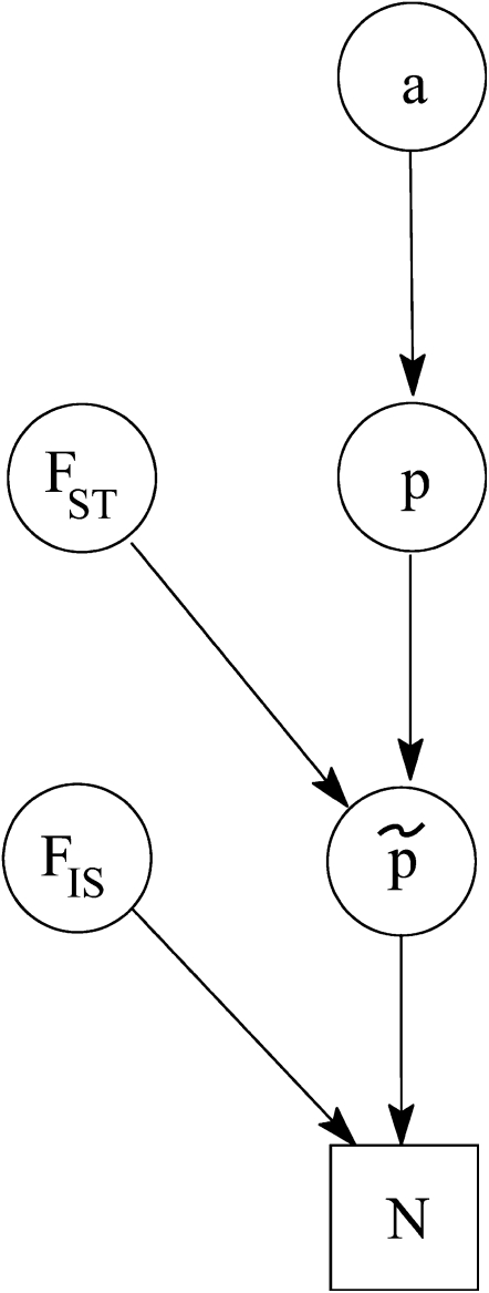
Up to here, our model differs from that of Holsinger et al. (2002) only in that we consider population-specific and parameters. We now introduce an additional modification by assuming a prior for the ancestral allele-frequency distributions that differs from the uniform used by them. More precisely, we use a beta(a, a) prior for every p_i, where a is a hyperparameter to estimate. The justification for this is Wright's (1931) observation that allele-frequency distributions for biallelic loci can be approached by such a distribution. With these assumptions, the posterior distribution of the full model represented by the directed acyclic graph (DAG) in Figure 2 is given by

(8)

Figure 2.—

DAG of the model given in Equation 8. The square node denotes known quantity (i.e., data) and circles represents parameters to be estimated. Lines between nodes represent direct stochastic relationships within the model. The variables within each node correspond to the different model parameters discussed in the text. N is the genetic data, is the vector of inbreeding coefficients, and are, respectively, the actual and ancestral allele frequencies, is the vector of the genetic differentiation coefficient for each local population, and a is the hyperprior determining the shape of the ancestral allele frequencies.

We take noninformative priors for every , and every . The parameter a is scaled between zero and infinity so we use a lognormal distribution as prior: a ∼ lognormal(0, 1). Note that priors for , , and are respectively given by the products of priors of p_i, , and . This Bayesian formulation was implemented using both a classical MCMC approach and the ABC approach proposed by Beaumont et al. (2002) and is described in detail below.

SOURCES OF BIAS

In what follows we describe two sources of bias that are introduced when analyzing AFLP data. The first one is due to the “noninformative” prior of the ancestral allele frequencies used in the original method (Holsinger et al. 2002), and the second one is due to the way markers included in the analysis are chosen (ascertainment bias). In what follows we explore the effects of these biases by comparing results given by an approximate Bayesian computation (ABC) implementation that does not correct for them with another one that does take them into account (this latter one is described in the solution: an abc approach).

Bias due to noninformative priors:

Holsinger et al. (2002) followed the common practice of using a flat prior on all ancestral allele frequencies p_i. In this model, as we explained above, the information on is contained in the shape of the genotype frequency distribution and so, even if a uniform prior is generally called “uninformative,” imposing here a flat prior leads to biased estimates if data sets (simulated or real) do not match this prior. Even if no information is available individually on frequencies, we have information on the general “shape” that allele frequencies should have in natural populations. As explained above, Wright (1931) showed that they can be approached by a beta distribution. For a single population (with no migration) and assuming low and symmetric mutation rates we obtain a “U-shaped” beta distribution with both parameters equal to 4Nμ < 1, where N is the effective size and μ is the mutation rate. With migration, and assuming that mutation is negligible, we obtain a uniform distribution if the migration rate m = 1/2N, a U-shaped beta distribution if m < 1/2N, and a bell-shaped beta otherwise. Thus, we use a beta prior for each p_i, i = 1, , I, with both parameters equal to a, which has to be estimated: p_i ∼ beta(a, a). We suppose that the distribution is symmetric, which is equivalent to assuming symmetric mutation rates and no selection. A more general prior would need a second parameter to estimate, but only little information is available on this hyperprior and so using a second parameter would lead to more uncertainty.

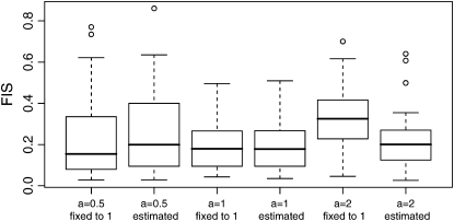
We illustrate the improvement of this new hyperprior by comparing the results of the full model introduced here, where a is estimated, with those of a model that uses the same uniform prior (a = 1) as in Holsinger et al. (2002). We consider a simple example with five populations and 100 loci, F_ST = 0.1, F_IS = 0.2, and 50 individuals in each population. We simulate 50 replicates of three different data sets: in the first one ancestral allele frequencies were simulated from beta(0.5, 0.5) (a = 0.5), in the second one from a uniform distribution (a = 1), and in the last one from a beta(2, 2) (a = 2) as in Holsinger et al. (2002). Results are presented in Figure 3 and were obtained using the software described below. We present results for only one of the five populations considered in our scenario because results for the remaining ones are very similar. First we observe that all box plots for F_IS where a is estimated by our method are centered around the true value of 0.2. In the case where allele frequencies are simulated from beta(2, 2) (a = 2) and a uniform prior is imposed, 's are overestimated around 0.33. The case where a = 0.5 seems to be less influenced by the uniform prior since F_IS is only weakly underestimated. As expected, when a = 1 the results are identical whether we estimate a or not because allele frequencies were simulated from a beta(1, 1) distribution. Finally when a is estimated, it appears that the accuracy of the estimates decreases as the parameter a decreases; this is discussed further below.

Figure 3.—

Box plot of the estimates of F_IS based on 50 replicates of three different data sets, depending on the value of the hyperprior parameter a using the full model presented in Figure 2 (a estimated) and the original model presented in Holsinger et al. (2002) with a flat hyperprior on ancestral allele frequencies (a fixed to 1). Data sets are based on five populations and 100 loci, F_ST = 0.1, and 50 individuals in each population; F_IS is fixed to 0.2. Boxes are constructed using the lower quartile and the upper quartile so that 50% of the values are in the boxes. The horizontal solid line in the box gives the median. The vertical dashed lines are called the “whiskers” and indicate the minimum and maximum values but only if they lie within 1.5 times the box height (the interquartile range). Points (solid circles) outside the whiskers are outlier values and are plotted.

Ascertainment bias:

Besides the bias due to the choice of prior, there are also important biases due to intrinsic properties of AFLP markers and to the way these markers are chosen.

An important property of AFLP markers is that if all individuals have the recessive [A2] phenotype, no band will be observed at all and we will not be able to identify this as a locus. As a result, we can never observe a locus i where all individuals have the [A2] phenotype; this corresponds to the case (we call this a hidden locus in the following). This is an intrinsic problem of AFLP markers and cannot be avoided. The second one is due to the way markers are chosen. In general, markers are not picked up at random and people prefer markers to be polymorphic with the intuition that they will give more information on genetic diversity. For example, Meudt and Clarke (2007, p. 106) in a review on AFLP markers suggest that “a marker must be polymorphic (i.e., show both plus and null alleles) to be informative.” It should be noted that what is called a fixed locus is a marker where all individuals have the same dominant [A1] phenotype and , but this can reflect different genotypes (A1A1 or A1A2). Excluding nonpolymorphic loci can dramatically change the shape of the phenotype distribution. This introduces a strong bias in the estimation of F_IS because, as discussed above and illustrated in Figure 1, the information on F_IS is contained in the shape of the phenotype distribution.

There is yet another ascertainment bias that is introduced when choosing the loci that will be used in the analyses. To distinguish artifacts from “real” bands, people often fix arbitrary minimum and maximum numbers of individuals with the dominant phenotype [A1] and choose only those loci for which the frequency of A1 lies within this interval. For example, some people exclude loci for which the frequency of the band is <1% or >99%. This procedure worsens the bias intrinsic to AFLPs that we described above. To incorporate it into the analysis, we introduce the notation hl (“hidden locus”) to identify the lower threshold and fl (“fixed locus”) to identify the upper threshold. Then, a locus i where is called a hidden locus (almost no individuals have the [A1] phenotype at locus i), and a locus i where is called a fixed locus (almost all individuals have the [A1] phenotype at locus i). Note that the intrinsic bias of AFLPs described at the beginning of this section sets a minimum lower bound of hl = 1.

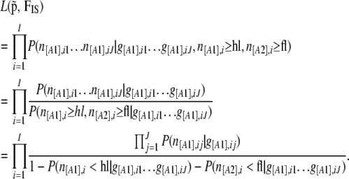
The first consequence of these biases is that the observed phenotype frequencies are not actually drawn from a binomial distribution as assumed by Equation 3. Faced with this, previous studies on single-nucleotide polymorphisms (SNPs) have modified the likelihood by conditioning on observing frequencies only between fixed bounds (Nicholson et al. 2002; Nielsen et al. 2004). Using the same approach, this time for phenotype frequencies rather than allele frequencies, we can rewrite the likelihood as

(9)

The numerator is then the same product of binomial distributions as in the original likelihood function and the denominator can be calculated by considering all the possible cases, for example, for hidden loci (we have similar equations for fixed loci):

with

And then is just a binomial density. This equation is a generalization of the truncated binomial likelihood used by Nielsen et al. (2004) and could be used in the context of a maximum-likelihood approach such as the one used by them for SNPs. However, as is shown in the appendix (G. Guillot, personal communication), it is not possible to use it in a hierarchical Bayesian approach. More specifically, if we follow Nicholson et al. (2002) and simply use this expression as our likelihood function in Equation 8, the ascertainment process is not correctly modeled. This is most conveniently explained by considering the following algorithm for generating a sample that conforms to the model above.

Algorithm 1:

1. Simulate a from lognormal(0, 1).

2. For each population j in 1 · · J,

   1. Simulate from .
   2. Simulate from and calculate .
3. For each locus i in 1 · · I,

   1. Simulate allele frequency p_i in the ancestral population from beta(a, a).
   2. For each population j in 1 · · J,

      1. Simulate allele frequency from beta(θ_jp_i, θ_j(1 − p_i)).
      2. Calculate phenotype frequency

         
   3. For each population j in 1 · · J,

      1. Simulate phenotype counts n_[A1],ij from binomial(n_[A1],ij, g_[A1],ij).
   4. If or if , go back to 3c.

This algorithm implies a rather peculiar model for discovering loci: if a locus does not conform to the discovery criteria it will be discarded, and the next locus will have exactly the same parametric population frequencies as the one discarded. This process will continue until a locus is accepted. Intuitively this is not a reasonable process. Rather, once a locus is discarded the next locus should be drawn with completely independent frequencies in all populations. Thus, at step 3d algorithm 1 should move to step 3a. Unfortunately, we have not been able to calculate the analytical expression (presented in the appendix) for this biologically more realistic ascertainment model, but demonstrate that this is possible using likelihood-free inference (Beaumont et al. 2002; Marjoram et al. 2003).

Two main problems arise from the use of the ascertainment model described by algorithm 1. First there is a violation of the assumption of statistical independence among the allele-frequency distributions of the different populations implicit in Equation 7, and, second, the ascertainment process modifies the distribution of ancestral allele frequencies.

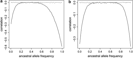
As an illustration of the first effect, for a given ancestral allele frequency, we can simulate a large number of replicates of allele frequencies and number of bands in actual populations from the exact model and then estimate the correlation coefficient between these sets of frequencies before and after having applied the ascertainment process described above with hl = 1 and fl = 1. We do this for F_IS = 0.1 and F_IS = 0.9 and two populations with 30 individuals and F_ST = 0.2 in each population. The effect of varying the number of populations and sample size is investigated later (see Sensitivity study). The correlation coefficients are plotted in Figure 4 against the value of the ancestral allele frequency. For unbiased data sets, the correlation is around zero because allele frequencies are independent in the two populations. But as expected, low and high ancestral allele frequencies produce a high correlation for biased data sets. For example, when the ancestral frequency is low (respectively high), if the allele frequency is close to zero (resp. one) in the first population, it is unlikely to be also close to zero (resp. one) in the second one because the locus was not hidden (resp. fixed).

Figure 4.—

Plot of the correlation coefficient between allele frequencies of two populations for unbiased (dashed lines) and biased (with hl = 1 and fl = 1, solid lines) data sets against the ancestral allele frequency. We simulated 30 individuals and F_ST = 0.2 in each population for F_IS = 0.1 (a) and F_IS = 0.9 (b).

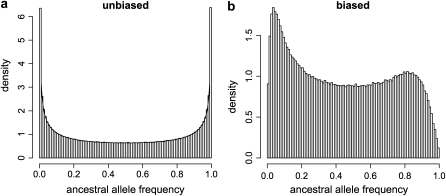
The second effect, the modification of the distribution of ancestral allele frequencies, arises because when we remove hidden and fixed loci, we remove at the same time the ancestral allele frequencies that produced them. For example, as hl increases (resp. fl), the probability of observing low (resp. high) ancestral allele frequencies decreases because they are more likely to produce hidden (resp. fixed) loci. As an illustration, with simulated data sets, we can draw the distribution of ancestral allele frequencies after having applied the ascertainment process because we know their true values. For this, we first simulate an unbiased large number of loci with ancestral allele frequencies drawn from a beta distribution with a = 0.5. Then for each locus, we simulate the allele frequencies in five populations with F_ST = 0.2 from the beta distribution of Equation 2. Finally for each locus in each population we draw the corresponding number of bands observed for 30 individuals and F_IS = 0.2 from the binomial distribution of Equation 3. By this way, we know for each locus the true value of allele frequencies in each population and in the ancestral population. After that, we remove all hidden and fixed loci from this data set using the ascertainment process described above with hl = 3 and fl = 3 to obtain a biased data set. This allows us to plot the distribution of ancestral allele frequencies in the biased data set because we know the true values of each ancestral allele frequency in this simulated data set (we do not need to estimate them). We plot these distributions for both unbiased and biased data sets in Figure 5. We can see that as expected, the loci with low and high frequencies are less likely to appear in the biased data set than in the original one.

Figure 5.—

Simulated distributions of ancestral allele frequencies for an unbiased data set (a) and a biased data set (b). The unbiased data were generated from the exact model with a = 0.5, five populations, 30 individuals, F_IS = 0.2, and F_ST = 0.2 in each population. Then we applied the ascertainment process to this data set using hl = 3 and fl = 3 to obtain the biased data set.

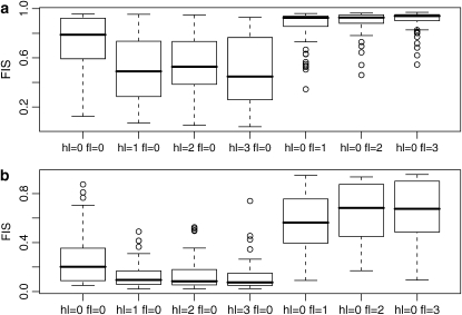
Ignoring these effects, and continuing to use the modified likelihood function, following the approach of Nicholson et al. (2002), leads to strong biases in estimation. We illustrate the influence of the bias using a typical example that may be problematic: we consider five populations, a sample size of 30 individuals per population, and a high differentiation coefficient F_ST = 0.25 in each one. Ancestral allele frequencies are simulated from a U-shaped beta distribution with parameter a = 0.7. We simulate two series of data sets: the first one with F_IS = 0.8 and the second one with F_IS = 0.2 in each population. To introduce the ascertainment bias, we imposed the constraint that at each locus there should be at least hl and at most fl individuals with the band, and we generated data sets with 100 loci. In each of the two series we simulated 50 replicates of different data sets with hl and fl varying independently from 0 to 3 (3 corresponds to 2% of the total number of 150 individuals). The results obtained for each of the five populations are very similar so we present the results for only one of them in Figure 6. When no bias is introduced by the exclusion of loci from the analysis (i.e., hl = 0 and fl = 0), the box plots are centered around the true values of 0.8 and 0.2. On the other hand, when hl is positive, F_IS is underestimated and when fl is positive, F_IS is overestimated. As expected, the bias is maximal for F_IS = 0.2 and hl > 0 because there is a very large number of fixed loci (see Figure 1). The bias is strong even for hl = 1 or fl = 1; however, increasing these values further has little effect on the estimates.

Figure 6.—

Comparison of the estimates of F_IS based on 50 replicates of different data sets with the ascertainment bias hl and fl varying independently from 0 to 3. Estimates are made under the assumption that there is no ascertainment bias (supposing that hl = 0 and fl = 0). (a) F_IS is fixed to 0.8; (b) F_IS is fixed to 0.2. Simulated data sets consist of five populations and 100 loci, F_ST = 0.25, and a sample size of 30 individuals per population.

THE SOLUTION: AN ABC APPROACH

The solution we propose to overcome the two biases described above is to use the ABC algorithm of Beaumont et al. (2002) instead of the classic MCMC scheme. The most valuable advantage of the ABC for our problem is that it does not require a closed form for the likelihood and internal priors (this allows us to include the ascertainment bias in the model). In addition, the ABC algorithm has the advantage of being highly parallelizable. This is an important consideration because of the emergence of multicore processors and the availability of calculation clusters. The ease with which the model is simulated and the fact that the ABC algorithm is highly parallelizable make the method proposed here very fast compared to the MCMC version and allow a very detailed sensitivity study.

The ABC algorithm is a rejection sampler: it generates data sets from given parameter values and accepts them when the simulated data set, D′, is “close” enough to the real data set, D. In the ABC framework, large data sets are reduced to a vector of summary statistics and close means that the Euclidian distance ‖·‖ between these statistics is below a given threshold value. If we assume that the real data set D follows a model M with parameters φ and use π(φ) to denote the prior density, the algorithm is given as follows.

Algorithm 2:

1. Choose a set of summary statistics S that will represent the data, and calculate s, the value of S for D.

2. Generate φ from priors π(·).

3. Simulate D′ from M with parameters φ and calculate s′, the value of S for D′.

4. Accept φ if and return to 2.

5. Stop when a sufficient number of data sets have been accepted.

The value of δ used in step 4 is pilot tuned in a shorter run using a target acceptance rate chosen by the user. For example, an acceptance rate of 0.01 means that the 1% of simulated s′ that are closest to s are accepted in step 4. Our approach also implements the local linear regression method proposed by Beaumont et al. (2002) that allows us to obtain accurate estimates using higher threshold values, δ and, therefore, decreases computation time. In our case, simulating from the model M is very easy, including simulating the biases discussed above. Note that the values of hl and fl need to be known. The complete algorithm for steps 2 and 3 in algorithm 2 is the one presented above (algorithm 1), with step 3d modified to move back to step 3a instead of step 3c to include the realistic ascertainment model we described.

In the ABC algorithm, the summary statistics are of primary importance and their choice determines directly the accuracy of the final results. Here we use different statistics to estimate and coefficients as proposed by Hamilton et al. (2005). Since the information about is contained in the shape of the phenotype frequency distribution of population j (see Introduction), we use the n-quantiles of these distributions as summary statistics for each population. They are representative values of the shape of a distribution: n points are taken at regular intervals from the cumulative distribution function. For example, the five 6-quantiles of the distributions presented in Figure 1 are, from left to right, (0.005, 0.06, 0.25, 0.57, 0.87), (0.04, 0.16, 0.38, 0.66, 0.90), and (0.07, 0.25, 0.50, 0.75, 0.93). These vectors reflect well that the first two distributions are skewed to the left (but the effect is less pronounced in the second case) and that the third distribution is symmetrical. In the context of the fission model (resp. island model), the measures how divergent each local population is from the ancestral population (resp. from the metapopulation as a whole). For this reason we calculate the global phenotype frequency at each locus i as and we define the observed phenotype differentiation for population j at locus i as

Then for each population j the summary statistics used are the n-quantiles of the distribution of Δ_ij among loci. If g_[A1],i = 0 we set Δ_ij = 0 because all populations will also have g_[A1],ij = 0.

Sensitivity study:

The method has been implemented in a software written in C++. We provide a command line version for both Linux and Microsoft Windows operating systems and a graphical user interface for the Windows version. The ABC algorithm is well adapted for parallel computing: with an acceptance rate of 0.005 and a sample size of 5000, the algorithm will simulate 1,000,000 independent data sets in steps 2 and 3. They can be generated independently on different computers or processors. We implemented the ABC algorithm on a computer cluster composed of 72 Itanium processors at 1.6 Ghz. As an example, it takes <15 sec for 48 processors to simulate 1,000,000 samples for a data set composed of five populations of 50 individuals and 100 loci. Multicore processors are now available on desktop computers and, for example, on a 2.66-Ghz quad core processor the same simulation would take <2 min. For each data set we present results based on 50 replicates of the same scenario.

We estimate parameters using 5000 independent samples from the ABC algorithm. We use the mode as a point estimate for the posterior distributions and estimate it using a Gaussian density kernel. Multiparameter least-squares fitting for the local linear regression is performed using the GNU Scientific Library (Galassi et al. 2006).

ABC algorithm parameters:

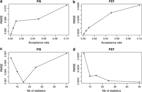
The algorithm we introduce requires the user to set the acceptance rate for the rejection algorithm. In general, smaller acceptance rates give more accurate results but also increase computation time because the user is forced to generate a larger number of data sets to obtain enough of them to estimate the parameters (Beaumont et al. 2002). Thus, it is important to investigate the influence of this parameter on the estimates. We simulated 50 synthetic data sets of five populations with 50 individuals per population, the same values of F_IS = 0.5 and F_ST = 0.15, and 200 loci. We estimated F_IS and F_ST parameters for each one of them using acceptance rates varying between 0.001 and 0.1. The results are illustrated in Figure 7, a and b, which shows the relative mean square error (RMSE) of the estimates of F_IS and F_ST for one of the populations against the acceptance rate. We calculated the RMSE using , where φ is either F_IS = 0.5 or F_ST = 0.15. As expected, a lower acceptance rate give lower RMSEs but the effect of this parameter is not very strong: multiplying the acceptance rate by 100 (0.001–0.1, which makes the calculation 100 time faster) increases the RMSE by only 16% for F_IS (from 0.061 to 0.071) and doubles the one of F_ST (0.03–0.06).

Figure 7.—

Plot of RMSE for estimates of F_IS and F_ST against the two parameters of the ABC algorithm: the acceptance rate and the number of quantiles used.

We also investigated the effect of the number of quantiles used for the summary statistics because it is known that in the ABC framework, using too many summary statistics can lead to a loss of accuracy (Hamilton et al. 2005). The problem lies in the fact that not all summary statistics provide information about the parameter being estimated. Since the distance used in the rejection step is based on all statistics, including many noninformative ones can mask the signal provided by informative statistics. Thus most of the variance of the distance measure used in the rejection step will consist of random noise introduced by the noninformative statistics. This in turn will increase the RMSE. Results are presented in Figure 7, c and d. The influence of the number of quantiles on RMSE is also small. Interestingly, for F_IS there is an optimal number of 15 quantiles while for F_ST RMSE decreases first very rapidly and then very slowly; not much is gained by using values >25. The different behavior is due to the fact that in the case of F_IS the information is contained in the shape of the phenotype frequency spectrum (see Figure 1 and the solution: an abc approach section) while in the case of F_ST it is contained in the shape of the distribution of phenotypic differentiation between local and ancestral populations (see the solution: an abc approach section). For the former, the distribution is bimodal while for the latter the distribution is unimodal (see supplemental material). Thus the number of quantiles that suffice to characterize these two distributions should certainly be different. To take into account this difference in behavior we always use 15 quantiles for the estimation of F_IS and 25 for the estimation of F_ST. Additionally, the threshold value δ was always tuned so as to obtain a target acceptance rate of 0.005.

Ascertainment bias:

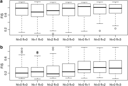
To show that the ABC algorithm can efficiently solve the problem posed by ascertainment bias, we use the same data sets used to plot Figure 6. The bias is corrected fairly well in all the scenarios we explored (Figure 8). The scenario hl = 0, fl = 0 represents the hypothetically unbiased case while hl = 1, fl = 0 represents the case where all observed markers are included in the analysis. All other scenarios represent cases where only polymorphic loci are considered; the only difference among them is the criteria used to decide if a locus is polymorphic or not. If F_IS is high (Figure 8a), our correction minimizes the loss of accuracy for the range of threshold values used for the minimum and maximum number of individuals with the dominant phenotype. However, if F_IS is low (Figure 8b), removing fixed loci for the dominant allele leads to a moderate loss of efficiency in our correction. Clearly, removing fixed loci in this latter case leads to a loss of information for F_IS estimation as expected from Figure 1. Note that the only intrinsic limitation of AFLP markers is hl ≥ 1; thus, this bias can be avoided simply by including all the fixed loci in the analyses.

Figure 8.—

Comparison of the estimates of F_IS based on the same simulated data sets presented in Figure 6. There are 50 replicates of different data sets with the ascertainment bias hl and fl varying independently from 0 to 3. Estimates are made taking into account the ascertainment bias in the ABC algorithm presented in the text. (a) F_IS is fixed to 0.8; (b) F_IS is fixed to 0.2. Data sets are based on five populations and 100 loci, F_ST = 0.25, and 30 individuals per population.

Size of the data set used:

We simulated many different data sets to investigate which kind of data set can give the best results with AFLPs. The starting point is a scenario with 100 loci, five populations, and 50 individuals per population. Then we modified each one of these parameters at a time and calculated the RMSE on the basis of 50 replicates of each data set. We fixed F_ST = 0.25 and F_IS = 0.5 in each population, and chose a = 0.7. We also included ascertainment bias with hl = 1 and fl = 0. We present the RMSEs for F_IS and F_ST for data sets containing 50–500 loci in Table 1. As expected, increasing the number of loci greatly reduces the RMSE. More precisely, the RMSE is reduced by a factor of 4.2 for F_IS and by a factor of 11.6 for F_ST.

TABLE 1.

The effect of the number of loci studied on the quality of the estimates: RMSE of the estimates of F_IS and F_ST using data sets with different numbers of loci

	No. of loci
	50	100	200	500
FIS	0.137	0.102	0.052	0.033
FST	0.0116	0.0044	0.0035	0.0010

Increasing the number of individuals per population is much less helpful than increasing the number of loci. There is no significant improvement for F_IS with 30, 50, or 100 individuals per population, and for F_ST the RMSE is reduced by only 30% (0.0073–0.0051; data not shown). Note that the fact that we have used equal sample sizes for all populations does not affect these results because we estimate population-specific F_ST's and F_IS's. Therefore, the sample size for population j should primarily influence the estimate for this population and not that of other populations. In terms of the number of populations considered, results for F_IS are similar, and the RMSE does not change much when the number of populations changes. However, the RMSE of F_ST is divided by 3 (0.0049–0.0016) when the number of populations is increased from 5 to 50 (data not shown). This can be easily explained by the fact that F_ST estimates are based on the estimation of the ancestral population (resp. metapopulation) allele frequencies, which are better estimated with a large number of populations.

Influence of biased F_IS estimations on F_ST coefficients:

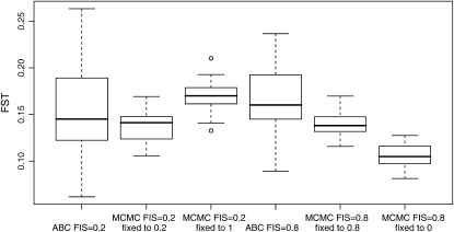
The biases we described above do not have a direct effect on F_ST estimates but they can influence them indirectly if they lead to highly biased estimates of F_IS simply because then allele frequency distributions will also be biased. To show this effect, we simulated 50 replicates of two data sets: one with F_IS = 0.2 and the other with F_IS = 0.8 in each population. For both scenarios the simulated data sets considered 200 loci, 10 populations, and 50 individuals per population, with a = 0.7 and F_ST = 0.15 in each population. For both scenarios we used the new ABC algorithm presented here where F_IS is estimated and an MCMC algorithm where instead of estimating F_IS we used a fixed value. We first fixed the value of F_IS to the true value (0.2 or 0.8) and then to the worst possible false value (1 for the case of F_IS = 0.2 and 0 for the case of F_IS = 0.8). Results are presented in Figure 9. It is clear that both the ABC algorithm and the MCMC algorithm with the correct value of F_IS give correct estimates of F_ST centered around the true value (0.15). However, the estimates of F_ST are clearly biased when using biased estimates of F_IS. F_ST is overestimated when F_IS is overestimated and F_ST is underestimated when F_IS is underestimated. Finally it is important to note that the ABC algorithm gives wider posterior density intervals for F_ST than the MCMC algorithm, but the latter can be used only if one knows the true value of F_IS.

Figure 9.—

Comparison of the estimates of F_ST based on 50 replicates of two data sets: one with F_IS = 0.2 and the other with F_IS = 0.8 in each population. We estimated F_ST with the ABC algorithm that estimates F_IS and with the MCMC algorithm with a fixed value of F_IS: either the true value or a false value.

DISCUSSION

In this article we identify two sources of bias that affect the estimation of F-statistics when using dominant markers and particularly AFLPs. More specifically, we show that when estimating inbreeding coefficients using dominant markers, (i) the use of MCMC techniques cannot take into account the ascertainment process, (ii) flat priors for allele-frequency distributions cannot be considered as noninformative, and (iii) monomorphic loci should be included in the analyses whenever this is possible. To avoid these biases, we presented a new statistical method based on the ABC algorithm. Additionally, our method estimates population-specific F_IS and F_ST coefficients and incorporates parameters to model ascertainment bias.

Our approach takes into account the fact that loci for which a band is not observed constitute hidden loci; it suffices to set hl = 1 (at least one individual has the band). Also, our study allows us to provide guidance to researchers developing AFLP markers. The common practice of excluding loci for which the frequency of the band is very low or very high should be avoided whenever possible. Sometimes it is necessary to impose stringent threshold values for technical reasons. For example, a locus will be included only if at least five individuals have the band (hl = 5) and at least five do not have it (fl = 5). In these cases, our method will still be capable of giving unbiased estimates (cf. Figure 8) but only if one knows the values of hl and fl that were used by the people developing AFLPs. Thus, it is very important to choose the conditions under which a given locus will be included in the analyses and then apply them in a consistent manner. These requirements may represent a problem when analyzing old data sets for which these values are not known. Thus, one desirable extension of our method would be to incorporate the uncertainty in hl and fl within the simulation step of the ABC algorithm. However, we note that doing this would lead to an increase in the RMSE of the estimations.

This article highlights the usefulness of the ABC algorithm for modeling ascertainment bias. We have demonstrated that a previous approach for modeling demographic history in structured populations (Nicholson et al. 2002) used formulas for taking into account ascertainment that are demonstrably problematic and do not conform to the underlying biological processes. Obtaining closed-form solutions for the biologically realistic ascertainment model can be very difficult. Using the ABC approach overcomes this problem and we demonstrate that this approach is particularly well adapted to incorporate the complex ascertainment biases observed for markers such as AFLPs and SNPs. It should be noted that in the case of Nicholson et al. (2002) the problem we have uncovered is unlikely to have a strong effect because they are dealing with codominant markers for which it is possible to easily estimate allele frequencies.

An important challenge posed by the use of ABC methods is finding sufficient summary statistics for the estimation of model parameters. In fact, no such statistics are usually available for population genetics applications but, encouragingly, near-sufficient statistics provide a reasonable approximation (Tavaré et al. 1997). In general, studies that use the ABC approach consider summary statistics such as the mean or the mode of a given parameter (e.g., F_ST, mean linkage disequilibrium between pairs of loci, average number of differences between pairs of DNA sequences, etc.). Here, we propose to use the quantiles of the summary statistic distributions across loci, because they provide much more information than the mean or the mode.

Many methods have been proposed to estimate the frequency of the null allele and the genetic diversity when using AFLP data (see Bonin et al. 2007 for a review) but all of them except that of Holsinger et al. (2002) assume Hardy–Weinberg equilibrium. It has been argued that doing this for AFLP markers when no information on F_IS is available is not a problem when comparing F_ST values across species or populations (Bonin et al. 2007). However, this is only the case if the level of inbreeding is the same for all species/populations. Otherwise, the magnitude of the bias will be different among them.

It should be noted that the model of Holsinger et al. (2002), as in the present article, implicitly assumes that the probability of observing a heterozygote at one locus in an individual, given F_IS and the allele frequencies, is independent of observing a heterozygote at another locus in the same individual. This will be true only if departures from Hardy–Weinberg are due to cryptic population structure (often termed the “Wahlund effect”) because, under a model of inbreeding, loci within an individual are not independent in their probability of heterozygosity. Indeed, it is possible to use this information to distinguish between the two potential causes of departure from Hardy–Weinberg (Overall and Nichols 2001).

Among all the existing methods dedicated to dominant markers, the model of Holsinger et al. (2002) is the only one that simultaneously estimates all parameters but, as we have shown, it is affected by the two sources of bias we have uncovered in this study. Our method, therefore, represents an important improvement over all existing ones and we expect that it will be of great help for the many researchers who are interested in using AFLP markers to study population structure.

APPENDIX

The correct algorithm for modeling ascertainment bias (where step 3d in text algorithm 1 sends us back to step 3a) can be described using a simplified notation. Let and , with . We also denote by A_i the set of all possible values for the vector that match the ascertainment condition (i.e., n_[A1],i < hl and n_[A2],i < fl).

Algorithm A:

1. Sample φ from f(φ).

2. For each locus i, while ,

   1. Sample ψ_i from g(ψ_i | φ).
   2. Sample from .

Algorithm A implies a full joint distribution for locus i, written as

where whenever the phenotypes match the ascertainment condition and 0 otherwise, and with

Then the marginal distribution of (φ, ψ_i) is

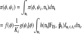This equation should be used as the full prior for (φ, ψ_i); the problem is that we have not been able to calculate the integral K_1,i, which in turn precludes us from using a MCMC approach.

The likelihood can indeed be calculated as

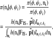which corresponds to the likelihood given in Equation 9 in the text.

References

- Balding, D. J., 2003. Likelihood-based inference for genetic correlation coefficients. Theor. Popul. Biol. 63 221–230. [DOI] [PubMed] [Google Scholar]
- Balding, D. J., and R. A. Nichols, 1995. A method for quantifying differentiation between populations at multi-allelic loci and its implications for investigating identity and paternity. Genetica 96 3–12. [DOI] [PubMed] [Google Scholar]
- Beaumont, M. A., and D. J. Balding, 2004. Identifying adaptive genetic divergence among populations from genome scans. Mol. Ecol. 13 969–980. [DOI] [PubMed] [Google Scholar]
- Beaumont, M. A., W. Y. Zhang and D. J. Balding, 2002. Approximate Bayesian computation in population genetics. Genetics 162 2025–2035. [DOI] [PMC free article] [PubMed] [Google Scholar]
- Bensch, S., and M. Akesson, 2005. Ten years of AFLP in ecology and evolution: Why so few animals? Mol. Ecol. 14 2899–2914. [DOI] [PubMed] [Google Scholar]
- Bonin, A., D. Ehrich and S. Manel, 2007. Statistical analysis of aflp data: a toolbox for molecular ecologists and evolutionists. Mol. Ecol. 16 3737–3758. [DOI] [PubMed] [Google Scholar]
- Ciofi, C., M. A. Beaumont, I. R. Swingland and M. W. Bruford, 1999. Genetic divergence and units for conservation in the Komodo dragon Varanus komodoensis. Proc. R. Soc. Lond. Ser. B Biol. Sci. 266 2269–2274. [Google Scholar]
- Excoffier, L., and G. Heckel, 2006. Computer programs for population genetics data analysis: a survival guide. Nat. Rev. Genet. 7 745–758. [DOI] [PubMed] [Google Scholar]
- Falush, D., M. Stephens and J. K. Pritchard, 2003. Inference of population structure using multilocus genotype data: linked loci and correlated allele frequencies. Genetics 164 1567–1587. [DOI] [PMC free article] [PubMed] [Google Scholar]
- Foll, M., and O. Gaggiotti, 2006. Identifying the environmental factors that determine the genetic structure of populations. Genetics 174 875–891. [DOI] [PMC free article] [PubMed] [Google Scholar]
- Galassi, M., J. Davies, J. Theiler, B. Gough, G. Jungman et al., 2006. GNU Scientific Library Reference Manual, Ed. 2. Network Theory Ltd., Bristol, UK.
- Gao, H., S. Williamson and C. D. Bustamante, 2007. An MCMC approach for joint inference of population structure and inbreeding rates from multilocus genotype data. Genetics 176 1635–1651. [DOI] [PMC free article] [PubMed] [Google Scholar]
- Hamilton, G., M. Currat, N. Ray, G. Heckel, M. Beaumont et al., 2005. Bayesian estimation of recent migration rates after a spatial expansion. Genetics 170 409–417. [DOI] [PMC free article] [PubMed] [Google Scholar]
- Hill, W. G., and B. S. Weir, 2004. Moment estimation of population diversity and genetic distance from data on recessive markers. Mol. Ecol. 13 895–908 (erratum in Mol. Ecol. 13: 3617). [DOI] [PubMed] [Google Scholar]
- Holsinger, K. E., P. O. Lewis and D. K. Dey, 2002. A Bayesian approach to inferring population structure from dominant markers. Mol. Ecol. 11 1157–1164. [DOI] [PubMed] [Google Scholar]
- Lynch, M., and B. G. Milligan, 1994. Analysis of population genetic-structure with rapd markers. Mol. Ecol. 3 91–99. [DOI] [PubMed] [Google Scholar]
- Marjoram, P., J. Molitor, V. Plagnol and S. Tavare, 2003. Markov chain Monte Carlo without likelihoods. Proc. Natl. Acad. Sci. USA 100 15324–15328. [DOI] [PMC free article] [PubMed] [Google Scholar]
- Meudt, H. M., and A. C. Clarke, 2007. Almost forgotten or latest practice? AFLP applications, analyses and advances. Trends Plant Sci. 12 106–117. [DOI] [PubMed] [Google Scholar]
- Nicholson, G., A. V. Smith, F. Jonsson, O. Gustafsson, K. Stefansson et al., 2002. Assessing population differentiation and isolation from single-nucleotide polymorphism data. J. R. Stat. Soc. Ser. B Stat. Methodol. 64 695–715. [Google Scholar]
- Nielsen, R., M. J. Hubisz and A. G. Clark, 2004. Reconstituting the frequency spectrum of ascertained single-nucleotide polymorphism data. Genetics 168 2373–2382. [DOI] [PMC free article] [PubMed] [Google Scholar]
- Overall, A. D. J., and R. A. Nichols, 2001. A method for distinguishing consanguinity and population substructure using multilocus genotype data. Mol. Biol. Evol. 18 2048–2056. [DOI] [PubMed] [Google Scholar]
- Tavaré, S., D. J. Balding, R. C. Griffiths and P. Donnelly, 1997. Inferring coalescence times from DNA sequence data. Genetics 145 505–518. [DOI] [PMC free article] [PubMed] [Google Scholar]
- Wright, S., 1931. Evolution in Mendelian populations. Genetics 16 97–159. [DOI] [PMC free article] [PubMed] [Google Scholar]
- Wright, S., 1951. The genetic structure of populations. Ann. Eugen. 15 323–354. [DOI] [PubMed] [Google Scholar]
- Zhivotovsky, L. A., 1999. Estimating population structure in diploids with multilocus dominant DNA markers. Mol. Ecol. 8 907–913. [DOI] [PubMed] [Google Scholar]