

Abstract
It has been proposed that VF waves emanate from stable localized sources, often called “mother rotors.” However, evidence for the existence of these rotors is conflicting. Using a new panoramic optical mapping system that can image nearly the entire ventricular epicardium, we recently excluded epicardial mother rotors as the drivers of Wiggers’ stage II VF in the isolated swine heart. Furthermore, we were unable to find evidence that VF requires sustained intramural sources. The present study was designed to test the following hypotheses: 1. VF is driven by a specific region, and 2. Rotors that are long-lived, though not necessarily permanent, are the primary generators of VF wavefronts. Using panoramic optical mapping, we mapped VF wavefronts from 6 isolated swine hearts. Wavefronts were tracked to characterize their activation pathways and to locate their originating sources. We found that the wavefronts that participate in epicardial reentry were not confined to a compact region; rather they activated the entire epicardial surface. New wavefronts feeding into the epicardial activation pattern were generated over the majority of the epicardium and almost all of them were associated with rotors or repetitive breakthrough patterns that lasted for less than 2 s. These findings indicate that epicardial wavefronts in this model are generated by many transitory epicardial sources distributed over the entire surface of the heart.
1. Introduction
During ventricular fibrillation, the myocardium is activated by a multitude of complexly interacting electrical wavefronts. A question that has received considerable recent attention is whether the sources of these wavefronts are short lived and widely distributed [1], or whether they are generated by one—or possibly a few—persistent localized sources [2–4]. The former scenario is the classic multiple wavelet mechanism and the latter is often called the mother rotor mechanism because permanent rotors are the putative driving sources. The distinction between the two broad mechanisms could be important to the design of new anti-VF therapies: if VF is locally driven, it might be possible to terminate it by targeting individual rotors or a limited part of the heart. On the other hand, a distributed mechanism suggests that more global interventions, such as defibrillation shocks, would be more effective.
A rotor is a reentrant wavefront that pivots about a point at its end. This pivot point, called a phase singularity (PS), is a point at which the wavefront is in contact with its own refractory wake [5, 6]. In 3D muscle, the singular point generalizes to a 1D filament that snakes through the tissue [5, 7]. The term phase singularity is often used interchangeably with wavebreak [8].
In a recent series of experiments, we used a new optical mapping system that can image nearly the entire ventricular epicardium [9, 10] and graph theoretic pattern analysis algorithms [11] to study early VF (~20 s post-induction) in isolated swine hearts. This time period is important clinically because it corresponds to therapy delivery by implantable defibrillators. We excluded epicardial mother rotors (i.e., stable rotors with filaments intersecting the epicardial surface) as the drivers of VF in this experimental model [10], and were additionally unable to find any evidence that VF is driven by intramural [12] mother rotors. Nevertheless, approximately 12 epicardial rotors of limited duration were present at any given time. A few of these rotors were relatively long-lived, sometimes lasting for seconds [10]. We further found that reentry on the epicardium was incessant, even though the reentry was not organized into persistent rotors [12]. We also observed relatively long-lived (though not generally permanent) breakthrough patterns that were consistent with the presence of intramural rotors [12].
We reasoned that if VF is not driven by mother rotors, then perhaps it is driven by “mother regions,” i.e., discrete regions that spawn wavefronts that expand outward and activate the remainder of the ventricles. We further reasoned that if permanent rotors are not the primary wavefront generators, then maybe rotors that are not permanent, yet still have very long lives, are. The present study addresses these two questions using new analyses of our previously collected VF data. We find that local regions do not drive VF in this model, and furthermore, that short-lived sources (i.e., epicardial rotors and repetitive breakthrough patterns) generate the great majority of wavefronts.
2. Methods
2.1 Animal Preparation and Data Collection
In this paper, we report further analysis of VF mapping data that were previously collected and partially analyzed [10, 12]. Animal preparation and data collection have been described in detail [10]. Briefly, we studied isolated, perfused hearts from six healthy, young, mixed breed pigs of either sex (weight: 23±4 kg). We studied a total of 17 VF episodes—three from each of five animals and two from the sixth. The hearts were stained with the potentiometric fluorescent dye di-4-ANEPPS. 2,3-butanedione monoxime (BDM, 20 mMol) was added to the perfusate to prevent the hearts from contracting. VF was induced by touching a 9-V battery to the right ventricular epicardium. We recorded VF patterns using a newly developed panoramic optical mapping system that can map from nearly the entire epicardial surface at ~1.6 mm spatial resolution and 750 frames/s [9, 10]. With this system, fluorescence is excited using 32 high-power light emitting diodes (470 nm) and recorded with 4 fast CCD video cameras through 590 nm longpass filters. The fluorescence consists of a large background signal upon which are superimposed small fluctuations inversely proportional to the transmembrane potential. The epicardial geometry is reconstructed from a series of images of the heart collected at 5° increments by a fifth video camera that rotates about the heart. The resulting model is a mesh of approximately equally-sized triangles spaced by ~1.6 mm (centroid-to-centroid). Background-subtracted fluorescence data from the four high-speed cameras are merged into a single continuous dataset by texture mapping the data onto the epicardial model. The signal associated with each mesh triangle is normalized to the range 0–100.
Each mapped VF episode was 4 s long. Datasets on the order of 4 s in length are typical in VF research [3, 13, 14]. Although our system can record continuously for minutes, in optical mapping, short runs are advantageous to minimize photodynamic effects such as photobleaching of the potentiometric dye. Our choice of 4-second runs is further justified by our finding that virtually all rotors had lifetimes much less than 4 s [10], showing that the mapping interval was longer than the lifetimes of the patterns of interest. Recording began approximately 20 s after VF induction, which corresponds to Wigger’s stage II VF. This stage of VF is commonly studied in in vivo experiments because it is the stage during which implantable defibrillators deliver therapy, and because experimental subjects without circulatory support will not survive if VF is allowed to continue for significantly longer. Optical mapping studies are often performed with ex vivo hearts that are continuously perfused. In these studies, it is not unusual for mapping to be delayed for several minutes after VF induction [3, 15, 16].
2.2 Wavefront and Rotor Identification
We processed the VF datasets using recently developed analysis algorithms that identify activation wavefronts and PSs and characterize their interrelationships [11]. Briefly, each normalized fluorescence signal is converted to phase [6]: First, we ensure that all action potentials oscillate about a mean of 0 by subtracting any beat-by-beat linear trends. This detrended signal is then plotted against its integral. Points associated with each temporal sample follow a trajectory that circles the origin of this phase plane. The phase value for each sample is found by converting the phase plane to a polar coordinate system and taking the angular coordinate of the point [11]. A major benefit of the phase representation of a signal is that phase has a unique value as a patch of tissue progresses through an action potential—this is in contrast to transmembrane potential, which has the same value twice during an action potential: once when depolarizing and again when repolarizing. This feature simplifies identification of wavefronts and PSs.
PSs are points surrounded by tissue with all possible phase values [5, 6]. Wavefronts are isolines of the phase value corresponding to the upstroke (−π/2). Wavefronts must either be closed loops, or be terminated in space by PSs or by boundaries [6]. Our previously described algorithms for tracking PSs and wavefronts [11] also identify which wavefronts are associated with specific PSs. It is possible for a rotating wave to switch from one PS to another as it circulates. We call such patterns compound rotors. Our previous publication details our method for identifying them [10].
The spatial resolution used in this study (~1.6 mm) has previously been shown to be optimal for characterizing VF patterns [17]. This spatial resolution, together with our temporal resolution of 1.33 ms, can reliably track wavefronts from frame-to-frame as long as the propagation speed at some point along the front is < ~120 cm/s. This is two to three times the propagation speed we have previously reported in this preparation during VF [18].
2.3 Wavefront Graphs
Our algorithms codify the timing of the wavefronts and their interrelationships using a type of directed graph [19] called a wavefront graph [11, 20]. Figure 1 shows a very simple example. In this representation, a wavefront is an arrow. The horizontal positions of an arrow’s initial and terminal endpoints specify the wavefront’s starting and ending times. The vertical positions are not significant. Wavefronts that are present at the beginning or end of mapping are assigned the starting or ending time of the episode. Wavefront fragmentations and collisions are frequent events during VF. A fragmentation is indicated by a wavefront branching into two (or more) new wavefronts. The terminal endpoint of the original wavefront is connected in the wavefront graph to the initial endpoints of the new wavefronts. Examples from Figure 1 are wavefront a fragmenting into wavefronts b and c and wavefront e fragmenting into wavefronts f and g. Conversely, a collision is indicated by two (or more) wavefronts coming together to form a new wavefront. In this case, the terminal endpoints of the original wavefronts are connected to the initial endpoint of the new wavefront. An example is wavefronts c and d combining into wavefront e. More complex events, in which multiple wavefronts come together with multiple new wavefronts emerging, are also possible. Our previous publications contain several additional simple examples of wavefront graphs [11, 12, 20, 21]. Reference [12] contains a complete wavefront graph derived from 1 s of panoramically mapped VF in the swine heart.
Figure 1.
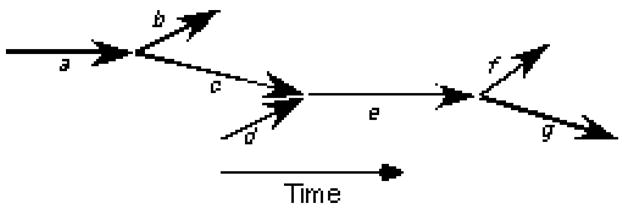
A simple wavefront graph. Each arrow represents a wavefront. The horizontal positions of a wavefront’s endpoints place the wavefront in time. The vertical positions are not significant. Wavefront a fragments into wavefronts b and c; wavefronts c and d collide and coalesce to form wavefront e, which later fragments into wavefronts f and g.
In Figure 1, all of the wavefronts are interconnected; however, this does not have to be the case. Suppose that after the termination of wavefront g, a second cycle of the same activation pattern took place. The two sets of wavefronts (each set containing 7 wavefronts and associated with one cycle) would form two independent subgraphs of the overall wavefront graph. Such subgraphs are called components.
2.4 Perennial Wavefronts
The starting time of a component is the starting time of the earliest wavefront in the component. More than one wavefront may share this starting time. One subset of wavefronts in the component consists of the earliest wavefront(s) and all of their descendents. By descendents, we mean the wavefronts that can be found by tracing forward in time through the wavefront graph. Such wavefronts are found by applying a standard depth-first search algorithm to the wavefront graph (In a depth-first search, “descendant” waves are visited before “sibling” waves; for example, in Figure 1, the depth-first search order starting at a is a-c-e-g-f-b [19].). Conversely, one or more wavefronts may share the ending time of the component. A second subset of the component’s wavefronts consists of these latest wavefront(s) and all of their ancestors. We call wavefronts that are in the intersection of these two subsets perennial wavefronts. The perennial wavefronts of a component are on one of the lines of succession that connect the earliest wavefronts to the latest. In the wavefront graph shown in Figure 1, all wavefronts except for d are in the first subset. All wavefronts except for b and f are in the second. Wavefronts a, c, e, and g are the perennial wavefronts.
2.5 Root Wavefronts
Because propagating wavefronts will eventually collide with either a boundary or another wavefront and be extinguished, for VF to continue, new wavefronts must continually be produced. From the perspective of epicardial mapping data, these new wavefronts can be generated by successive cycles of epicardial reentry or appear de novo on the epicardium. In the later case, the wavefronts could derive either from intramural reentry or from true foci. We term these new wavefronts root wavefronts (RWs) because the remaining wavefronts in the overall epicardial activation pattern descend from them. We define two types of RWs: Rotor RWs are wavefronts attached to a PS that has a lifetime of at least 200 ms. We use a lower bound on PS lifetime to eliminate very short-lived PSs that are likely due to noise in the optical recordings; PSs lasting longer than 200 ms have completed at least one cycle of reentry. Breakthrough RWs are wavefronts that appear de novo on the epicardium. RWs are propagating wavefronts, and as such, occupy a finite area of the epicardium that changes from frame to frame. However, for some of our analyses, it is useful to assign a single epicardial site to each RW to represent its position. We term these sites root sites. For a rotor RW, the root site is defined as the position of the PS in the last frame of the wavefront; for a breakthrough RW, the root site is defined as the first site identified as part of the wavefront in its first temporal frame [11].
Each RW is said to contribute to all of the wavefronts that can be reached from it by tracing forward in time through the wavefront graph. During VF, each wavefront is usually contributed to by many RWs. To determine the set of RWs that contribute to each wavefront, we first create an empty set (i.e., an empty container) of contributing RWs for each wavefront. We then iterate over all RWs in the wavefront graph and for each determine the wavefronts that can be reached from it using a standard depth-first search algorithm [19]. This RW is then added to the contributing RW set of all the wavefronts that were reached. For example, in Figure 1, wavefronts a and d are RWs. Wavefronts b, c, e, f, and g can be reached from RW a and wavefronts e, f, and g can be reached from RW d. Wavefronts e, f and g have both RW a and RW d in their contributing RW set; wavefronts b and c have only RW a in their contributing RW set.
2.6 Characteristic Length
In some of our analyses, we are interested in how widely (or narrowly) a set of sites is scattered over the epicardium. We therefore defined a characteristic length (ChL) parameter that can be computed for any set of sites (i.e., triangles) in the mesh that makes up an epicardial geometry. ChL is simply an average distance between sites: if the sites are widely scattered, ChL will be larger than if they are narrowly scattered. To compute ChL, we first identify all unique pairs of sites in the set. This is the first site paired with each of the others, the second site paired will all but the first, the third site paired with all but the first and second, and so forth. We then estimate the length of the geodesic line that joins the two sites in each pair. A geodesic line is the shortest line between two points that runs over the surface. Because all triangles in the model are approximately equal in size, the length of a geodesic is approximately equal to the minimum number of triangle-to-triangle steps needed to reach the second site from the first, multiplied by the model’s average centroid-to-centroid triangle spacing. This spacing is typically ~1.6 mm. We find the minimum number of steps between two sites using a standard breadth-first graph search algorithm [19]. In such a search, the first site’s three immediate neighbors are examined to see if one of them is the second site. If none of them is, the sites neighboring those three sites are checked next. This process continues—with all sites in a level of neighbors being checked before descending to the next level of neighbors—until the second site is found. Once the inter-site distance for all pairs has been found, ChL is computed as the average distance.
Because ChL is a linear dimension, it is a function of both the area and shape of the region spanned by a set of sites. For example, a set of sites uniformly distributed over a rectangle will have a larger ChL than the same sites distributed over a square of the same area. ChL is also a function of the distribution of sites. If sites are concentrated near the center of a region, ChL will be smaller than if the sites were concentrated near the region’s perimeter. To illustrate some values of ChL, we computed ChL using: 1. all of the sites in an epicardial model (Figure 2A); 2. the sites on one side of a longitudinal cutting plane running approximately through the apex of the same model (Figure 2B); and 3. the sites on the apical side of a transverse cutting plane approximately midway between apex and base (Figure 2C). These geometries contained 4326, 2387, and 2233 triangles, respectively (because all triangles are similar in size, the surface area of a model is proportional to the number of triangles). The ChL values were 34.04 mm, 26.61 mm, and 22.89 mm, respectively. Note that because of the shape dependence of ChL, the ChLs of the models in panels B and C are not well predicted by their area relative to the model in panel A.
Figure 2.
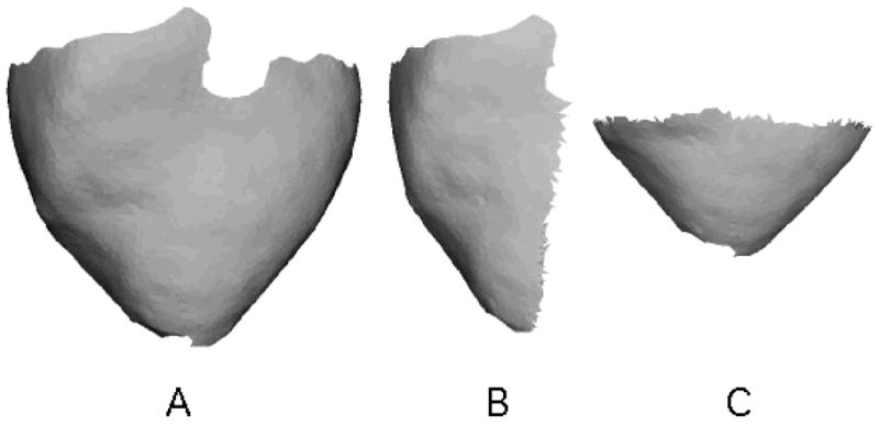
Geometric models used to compute ChL. A. Complete epicardial model. B. Lateral half of the model in A. C. Apical half of the model in A. These geometries contained 4326, 2387, and 2233 triangles, respectively. The ChL values were 34.04 mm, 26.61 mm, and 22.89 mm, respectively.
The ChL of a large set of sites can be accurately approximated by the ChL of a random sample of the sites. To show this, we computed the ChL of sets of sites containing 100, 250, 500, 1000, 2000, or 4000 sites randomly selected from the epicardial model shown in Figure 2a. We used 10 trials for each set size. By one-way ANOVA, set size had no effect on ChL (p>0.6; Figure 3).
Figure 3.
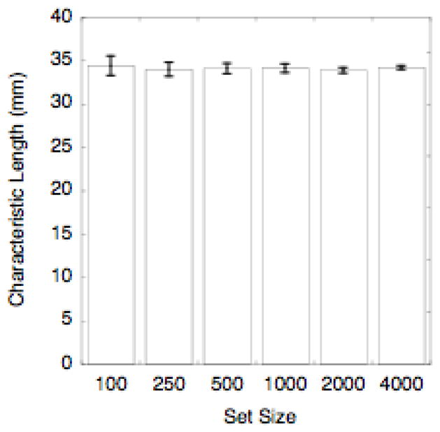
Independence of characteristic length on the size of the set used to compute it. The bars show characteristic length averaged over 10 trials for each set size. The error bars are standard deviations. There was no significant difference between groups (p>0.6). The ChL of the full set from which the test samples were drawn was 34.04 mm.
3. Results
We studied a total of 17 VF episodes from 6 animals. An example of the fluorescence data from one VF episode texture mapped onto the associated epicardial model is available as Video 1 in the online supplement to our previous publication [10]. Video 2 from the same paper animates the wavefronts and phase singularities found in this episode. We previously showed that these VF episodes contained 42,841±13,074 wavefronts (range: 18,162–74,215). Furthermore, the wavefront graphs from all 17 VF episodes each contained a dominant component that contained 92%±1% of wavefronts and was responsible for 98%±1% of site activations. In all cases, the dominant component persisted from the beginning to the end of the mapped interval, indicating that complete reentrant pathways were continuously present on the epicardium [12] —even though these pathways were not organized as epicardial rotors [10].
For the present analysis, we identified the set of perennial wavefronts from the dominant component in each VF episode. Figure 4 shows snapshots of wavefronts (isolines of the phase value −π/2) identified by our algorithms [11]. The snapshots are all from the same VF episode and are separated by 1 s. The heart’s geometry is displayed with a Hammer map projection so that the entire epicardium can be seen. Perennial wavefronts are cyan, the remaining wavefronts in the dominant component are yellow, and wavefronts from other components are red. At all time points, the perennial wavefronts—the wavefronts that participate in continuous epicardial reentry—are spread over the entire epicardium. This is more evident in Movie 1, which animates this entire episode in the same format. Movie 2 is an additional example from a different heart.
Figure 4.
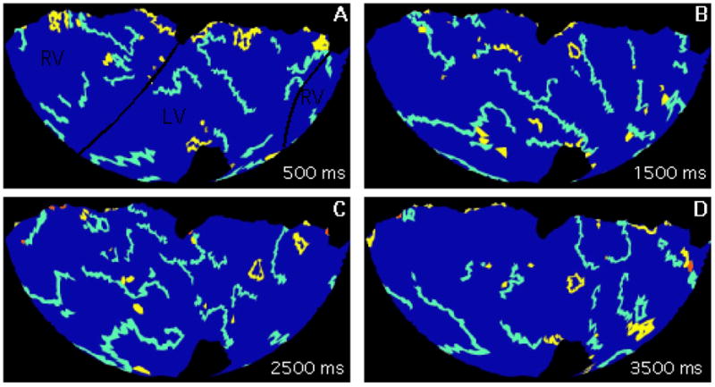
Wavefronts during VF. Snapshots are from the same episode and are separated by 1 s. The geometry is displayed with a Hammer map projection so that the entire epicardium is visible. The black lines in panel A indicate the approximate boundaries between the right and left ventricles. The wide colored lines are wavefronts: the perennial wavefronts are cyan, the remaining wavefronts from the dominant component are yellow, and wavefronts from other components are red. The entire 4-second episode is animated in supplemental movie S1.
To quantify the epicardial extent of the perennial wavefronts, for each VF episode, we computed how many triangles in the epicardial model that were ever activated by any wavefront were also activated at least once by a perennial wavefront. In all 17 episodes, essentially all sites were activated by the perennial wavefronts (99.87% ± 0.004%).
Of all the wavefronts, 27%±4% were RWs (range 22%–36%). Rotor RWs were 35% ± 12% of all RWs (range 15%–59%). The remaining RWs were breakthrough RWs. As an index of the epicardial span of the RWs, we computed the ChL of the root sites in each episode. We then normalized this ChL by the ChL of all sites in the associated epicardial geometry. If the root sites are a random sample of all of the epicardial sites, then the normalized root site ChL will be close to 1 (Figure 3). Conversely, if the root sites are clustered in particular regions, the normalized root site ChL will be closer to 0. We found that normalized root site ChL was 0.96±0.04 (range: 0.89 to 1.01), which indicates that the root sites were scattered over nearly the entire epicardium. Figure 5 shows the distribution of all root sites in one VF episode. The normalized root site ChL in this case was 0.96.
Figure 5.
Distribution of root sites (white triangles) from one VF episode. Some white triangles may have been the root site for more than one root wavefront. The geometry is displayed with a Hammer map projection. The anatomic orientation is similar to Figure 4. The normalized source site ChL is 0.96.
We identified the set of RWs that contributed to each individual wavefront. We then computed the ChL of the root sites for each such set. These quantities were called wavefront ChLs. We found the weighted average of the wavefront ChLs in each episode. For this calculation, the weight was the size of the associated wavefront, where size was defined as the sum of the number of sites the wavefront occupied in each frame. The average wavefront ChL was then normalized by the episode’s root site ChL. This quantity was 0.93±0.02 (range: 0.90–0.98). This large value indicates that the RWs contributing to each individual wavefront spanned nearly the same epicardial area as the set of all RWs in the episode.
We classified each rotor RW as arising from a compound rotor [10] that was either short-lived (< 2 s, which is half the mapped interval) or long-lived (>= 2s). The fraction of rotor RWs associated with long-lived rotors was only 0.07 ± 0.13 (range: 0.0–0.5). In other words, almost all wavefronts spawned by epicardial rotors came from short-lived rotors. We also identified repetitive breakthrough patterns that lasted for at least 2 s without significant shift of the epicardial breakthrough site [10, 12]. The fraction of breakthrough RWs associated with these long-lasting breakthrough patterns was nearly 0 (0.002 ± 0.003; range 0.0–0.011). Thus, breakthrough wavefronts could arise anywhere on the epicardium at any time without association with long-term repetitive patterns.
4. Discussion
The question of whether VF is driven by a stable, localized periodic source has been controversial in recent years. The evidence for local drivers is strongest in hearts from small animals [2, 3], however, investigators from a different laboratory using a very similar experimental preparation were unable to reproduce these findings [15, 22]. One possible explanation for the discrepancy is that the perfusate in the studies that found stable drivers could have had reduced osmolarity, which could have modulated action potential duration through activation of chloride channels, thereby transforming multiple wavelet VF to highly-organized, locally driven VF [23]. Such VF is sometimes called type II VF and can be induced by interventions that flatten action potential duration restitution and depress excitability [24]. In hearts more comparable in size to human hearts, some investigators have reported evidence for persistent periodic drivers. However, this evidence is indirect [4, 25] or obtained with relatively low spatial resolution [26]. A number of other studies have specifically sought reentry during VF but have not found clear evidence for mother rotors [14, 21, 27–33]. However, those studies mapped limited regions, admitting the possibility that such drivers were present, but located in an unmapped part of the heart. Both sets of studies employed a mixture of species (sheep, dog and pig), heart preparations (in vivo, isolated perfused), and recording modalities (electrical, optical) indicating that the existence of evidence for mother rotors is not solely a function of experimental model.
To determine if previous failures to find mother rotors were simply the result of looking in the wrong place, we mapped stage II VF in isolated perfused swine hearts using a newly developed panoramic optical mapping system that can image essentially the entire epicardium with ~1.5mm spatial resolution. We found that rotors are present in the isolated swine heart preparation with about a dozen whose lifetimes exceed 200 ms being present at any given time. However, although each VF episode had at least one rotor that lasted for 1 s or longer, only one of 17 episodes contained rotors that persisted for the entire 4-s mapped interval. We therefore excluded stable, persistent epicardial rotors as the drivers of VF in this model [10]. In a subsequent paper, using graph theoretic analysis of the same VF datasets, we sought evidence that sources hidden within the heart wall were required to maintain epicardial activation. We were unable to find such evidence, instead finding that reentrant pathways visible on the epicardium were always present and therefore sufficient to maintain activation [12].
The lack of evidence for mother rotors in this experimental model led us to ask two related questions for the present study: First, is VF driven by a particular region, even if the region does not necessarily contain a mother rotor? Our data show that the answer is no. We found that the perennial wavefronts—the wavefronts that participate in incessant epicardial reentry—were not confined to a compact region; rather, they activated the entire epicardium. If VF were driven by a limited region, we would expect to see the perennial wavefronts confined to that region with non-perennial wavefronts spreading outward as predicted by the mother rotor hypothesis [2]. Furthermore, the root sites—the epicardial sites associated with new wavefronts that feed into the epicardial activation pattern—were distributed over nearly the entire epicardium. In addition, the characteristic length of the root sites associated with individual wavefronts (wavefront ChL) was close to 1, indicating that individual wavefronts descended from root wavefronts distributed over almost all of the epicardium and not solely from localized root wavefronts.
The second question relates to the relative importance of long-lived rotors (and repetitive breakthrough patterns, which are consistent with intramural rotors). Could such sources be the primary generators of wavefronts, even though they are not true mother rotors in the sense that they are not permanent? Again the answer is no. Almost all the root wavefronts, both rotor RWs and breakthrough RWs, were associated with driving patterns less than 2 s in duration (93%±0.13% and 99.8%±0.3%, respectively).
The picture that emerges from these data is that early VF in this experimental model is driven by a multitude of transient sources distributed throughout the heart. Although long-lived sources are present, they are not the primary wavefront generators. This suggests that new anti-VF treatments designed to target individual rotors or limited parts of the heart may be less effective than more global interventions.
These patterns are broadly consistent with mapping studies of VF in human hearts. Wu et al. [34] mapped a limited (32mm × 38mm) epicardial region of isolated human hearts explanted from transplant recipients. Nanthakumar et al. [35] mapped a similarly sized region of in situ hearts of patients undergoing cardiac surgery. Both studies found that while reentry was present, it typically lasted only a few cycles. Nash et al. mapped VF patterns in patients undergoing cardiac surgery using 256 electrodes spanning the entire epicardium. They reported that VF at times appeared to be driven by a single rotor, but that this pattern was not persistent and that stable rotors were not the sole drivers of VF [36]. In a similar mapping study of patients with cardiomyopathy, Masse et al. found that rotors were present in all hearts studied, but all had limited lifetimes, with the longest in each episode lasting about 2 s. Overall, VF in human hearts appears to feature larger wavefronts and simpler patterns than VF in swine. This is borne out by a recent whole-heart computer modeling study of human VF that produced VF patterns that were markedly simpler than those typically observed in large animal studies [37].
Limitations
The study focused on Wiggers’ stage II VF in hearts isolated from healthy young pigs. Because activation patterns are known to change as VF proceeds [16, 32], VF characteristics could be different at different times in VF. VF characteristics may also be different in the presence of pathologies such as ischemia or infarction when fixed heterogeneities may play a more prominent role in VF maintenance [38]. In our study, the hearts were exposed to BDM to eliminate motion artifacts in the optical recordings. We previously found that VF patterns in this preparation are slower and more regular than those in the same hearts before excision [18]. Other authors have found that BDM converts VF to a stable tachycardia in isolated ventricular tissue from dogs [39] and pigs [40]. Evans et al. used BDM to stabilize reentry to create a model of monomorphic ventricular tachycardia in rabbit hearts [41]. Thus, although BDM almost certainly affected VF patterns, it is likely that in the absence of BDM, VF wavefront sources would have been even more unstable and transitory than what we observed.
Supplementary Material
Movies 1 and 2 animate wavefronts identified and classified by our algorithms during VF. Each movie shows a different episode. The perennial wavefronts are cyan, the remaining wavefronts from the dominant component are yellow, and wavefronts from other components are red. The geometry is displayed with a Hammer map projection. Figure 4 in the main manuscript shows four frames from Movie 1. (QuickTime; 8 MB)
Acknowledgments
We thank C. Killingsworth, F. Vance, and R. Collins for veterinary support. Supported in part by NIH grants HL-64184 (JMR) HL-28429 (REI) and a research grant from the Whitaker Foundation (MWK).
References
- 1.Moe GK, Reinboldt WC, Abildskov JA. A computer model of atrial fibrillation. American Heart Journal. 1964;67:200–20. doi: 10.1016/0002-8703(64)90371-0. [DOI] [PubMed] [Google Scholar]
- 2.Chen J, Mandapati R, Berenfeld O, Skanes AC, Jalife J. High frequency periodic sources underlie ventricular fibrillation in the isolated rabbit heart. Circulation Research. 2000;86:86–93. doi: 10.1161/01.res.86.1.86. [DOI] [PubMed] [Google Scholar]
- 3.Samie FH, Berenfeld O, Anumonwo J, Mironov SF, Udassi S, Beaumont J, Taffet S, Pertsov AM, Jalife J. Rectification of the Background Potassium Current: A Determinant of Rotor Dynamics in Ventricular Fibrillation. Circulation Research. 2001;89:1216–23. doi: 10.1161/hh2401.100818. [DOI] [PubMed] [Google Scholar]
- 4.Zaitsev AV, Berenfeld O, Mironov SF, Jalife J, Pertsov AM. Distribution of excitation frequencies on the epicardial and endocardial surfaces of fibrillating ventricular wall of the sheep heart. Circulation Research. 2000;86:408–17. doi: 10.1161/01.res.86.4.408. [DOI] [PubMed] [Google Scholar]
- 5.Winfree AT. When Time Breaks Down. Princeton: Princeton University Press; 1987. [Google Scholar]
- 6.Gray RA, Pertsov AM, Jalife J. Spatial and temporal organization during cardiac fibrillation. Nature. 1998;392:75–8. doi: 10.1038/32164. [DOI] [PubMed] [Google Scholar]
- 7.Pertsov AM. Scroll waves in three dimensions. In: Zipes DP, Jalife J, editors. Cardiac Electrophysiology, From Cell to Bedside. Philadelphia: W.B. Saunders; 2004. pp. 345–54. [Google Scholar]
- 8.Liu YB, Peter A, Lamp ST, Weiss JN, Chen PS, Lin SF. Spatiotemporal correlation between phase singularities and wavebreaks during ventricular fibrillation. Journal of Cardiovascular Electrophysiology. 2003;14 doi: 10.1046/j.1540-8167.2003.03218.x. [DOI] [PubMed] [Google Scholar]
- 9.Kay MW, Amison PM, Rogers JM. Three-dimensional surface reconstruction and panoramic optical mapping of large hearts. IEEE Transactions on Biomedical Engineering. 2004;51:1219–9. doi: 10.1109/TBME.2004.827261. [DOI] [PubMed] [Google Scholar]
- 10.Kay MW, Walcott GP, Gladden JD, Melnick SB, Rogers JM. Lifetimes of epicardial rotors in panoramic optical maps of fibrillating swine ventricles. Am J Physiol Heart Circ Physiol. 2006;291:H1935–1. doi: 10.1152/ajpheart.00276.2006. [DOI] [PMC free article] [PubMed] [Google Scholar]
- 11.Rogers JM. Combined phase singularity and wavefront analysis for optical maps of ventricular fibrillation. IEEE Transactions on Biomedical Engineering. 2004;51:56–65. doi: 10.1109/TBME.2003.820341. [DOI] [PubMed] [Google Scholar]
- 12.Rogers JM, Walcott GP, Gladden JD, Melnick SB, Kay MW. Panoramic optical mapping reveals continuous epicardial reentry during ventricular fibrillation in the isolated swine heart. Biophysical Journal. 2007;92:1090–5. doi: 10.1529/biophysj.106.092098. [DOI] [PMC free article] [PubMed] [Google Scholar]
- 13.Choi BR, Salama G. Simultaneous maps of optical action potentials and calcium transients in guinea-pig hearts: mechanisms underlying concordant alternans. Journal of Physiology. 2000;529(Pt 1):171–88. doi: 10.1111/j.1469-7793.2000.00171.x. [DOI] [PMC free article] [PubMed] [Google Scholar]
- 14.Rogers JM, Huang J, Melnick SB, Ideker RE. Sustained reentry in the left ventricle of fibrillating pig hearts. Circulation Research. 2003;92:539–45. doi: 10.1161/01.RES.0000061569.23879.20. [DOI] [PubMed] [Google Scholar]
- 15.Choi BR, Liu T, Salama G. The distribution of refractory periods influences the dynamics of ventricular fibrillation. Circulation Research. 2001;88:E49–58. doi: 10.1161/01.res.88.5.e49. [DOI] [PubMed] [Google Scholar]
- 16.Witkowski FX, Leon LJ, Penkoske PA, Giles WR, Spano ML, Ditto WL, Winfree AT. Spatiotemporal evolution of ventricular fibrillation. Nature. 1998;392:78–82. doi: 10.1038/32170. [DOI] [PubMed] [Google Scholar]
- 17.Bayly PV, Johnson EE, Idriss SF, Ideker RE, Smith WM. Efficient electrode spacing for examining spatial organization during ventricular fibrillation. IEEE Transactions on Biomedical Engineering. 1993;40:1060–6. doi: 10.1109/10.247805. [DOI] [PubMed] [Google Scholar]
- 18.Qin H, Kay MW, Chattipakorn N, Redden DT, Ideker RE, Rogers JM. Effects of heart isolation, voltage-sensitive dye, and electromechanical uncoupling agents on ventricular fibrillation. American Journal of Physiology Heart and Circulatory Physiology. 2003;284:H1818. doi: 10.1152/ajpheart.00923.2002. [DOI] [PubMed] [Google Scholar]
- 19.Chachra V, Ghare PM, Moore JM. Applications of Graph Theory Algorithms. New York: North Holland; 1979. [Google Scholar]
- 20.Rogers JM, Usui M, KenKnight BH, Ideker RE, Smith WM. A quantitative framework for analyzing epicardial activation patterns during ventricular fibrillation. Annals of Biomedical Engineering. 1997;25:749–60. doi: 10.1007/BF02684159. [DOI] [PubMed] [Google Scholar]
- 21.Rogers JM, Huang J, Smith WM, Ideker RE. Incidence, evolution, and spatial distribution of functional reentry during ventricular fibrillation in pigs. Circulation Research. 1999;84:945–54. doi: 10.1161/01.res.84.8.945. [DOI] [PubMed] [Google Scholar]
- 22.Choi BR, Nho W, Liu T, Salama G. Life span of ventricular fibrillation frequencies. Circulation Research. 2002;91:339–45. doi: 10.1161/01.res.0000031801.84308.f4. [DOI] [PubMed] [Google Scholar]
- 23.Choi BR, Hatton WJ, Hume JR, Liu T, Salama G. Low osmolarity transforms ventricular fibrillation from complex to highly organized, with a dominant high frequency source. Heart Rhythm. 2006 doi: 10.1016/j.hrthm.2006.06.026. In press. [DOI] [PubMed] [Google Scholar]
- 24.Wu TJ, Lin SF, Weiss JN, Ting CT, Chen PS. Two types of ventricular fibrillation in isolated rabbit hearts: importance of excitability and action potential duration restitution. Circulation. 2002;106:1859–66. doi: 10.1161/01.cir.0000031334.49170.fb. [DOI] [PubMed] [Google Scholar]
- 25.Thomas SP, Thiagalingam A, Wallace E, Kovoor P, Ross DL. Organization of myocardial activation during ventricular fibrillation after myocardial infarction: evidence for sustained high-frequency sources. Circulation. 2005;112:157–63. doi: 10.1161/CIRCULATIONAHA.104.503631. [DOI] [PubMed] [Google Scholar]
- 26.Everett TH, Wilson EE, Foreman S, Olgin JE. Mechanisms of ventricular fibrillation in canine models of congestive heart failure and ischemia assessed by in vivo noncontact mapping. Circulation. 2005;112:1532–41. doi: 10.1161/CIRCULATIONAHA.104.521351. [DOI] [PMC free article] [PubMed] [Google Scholar]
- 27.Huang J, Walcott GP, Killingsworth CR, Melnick SB, Rogers JM, Ideker RE. Quantification of activation patterns during ventricular fibrillation in open-chest porcine left ventricle and septum. Heart Rhythm. 2005;2:720–8. doi: 10.1016/j.hrthm.2005.03.025. [DOI] [PubMed] [Google Scholar]
- 28.Nanthakumar K, Huang J, Rogers JM, Johnson PL, Newton JC, Walcott GP, Justice RK, Rollins DL, Smith WM, Ideker RE. Regional differences in ventricular fibrillation in the open-chest porcine left ventricle. Circulation Research. 2002;91:733–40. doi: 10.1161/01.res.0000038945.66661.21. [DOI] [PubMed] [Google Scholar]
- 29.Rogers JM, Huang J, Pedoto RW, Walker RG, Smith WM, Ideker RE. Fibrillation is more complex in the left ventricle than the right ventricle. Journal of Cardiovascular Electrophysiology. 2000;11:1364–71. doi: 10.1046/j.1540-8167.2000.01364.x. [DOI] [PubMed] [Google Scholar]
- 30.Valderrabano M, Lee MH, Ohara T, Lai AC, Fishbein MC, Lin SF, Karagueuzian HS, Chen PS. Dynamics of intramural and transmural reentry during ventricular fibrillation in isolated swine ventricles. Circulation Research. 2001;88:839–48. doi: 10.1161/hh0801.089259. [DOI] [PubMed] [Google Scholar]
- 31.Huang J, Rogers JM, Killingsworth CR, Walcott GP, KenKnight BH, Smith WM, Ideker RE. Improvement of defibrillation efficacy and quantification of activation patterns during ventricular fibrillation in a canine heart failure model. Circulation. 2001;103:1473–8. doi: 10.1161/01.cir.103.10.1473. [DOI] [PubMed] [Google Scholar]
- 32.Huang J, Rogers JM, Killingsworth CR, Singh KP, Smith WM, Ideker RE. Evolution of activation patterns during long-duration ventricular fibrillation in dogs. Am J Physiol Heart Circ Physiol. 2004;286:H1193–200. doi: 10.1152/ajpheart.00773.2003. [DOI] [PubMed] [Google Scholar]
- 33.Lee JJ, Kamjoo K, Hough D, Hwang C, Fan W, Fishbein MC, Bonometti C, Ikeda T, Karagueuzian HS, Chen PS. Reentrant wave fronts in Wiggers’ stage II ventricular fibrillation. Characteristics and mechanisms of termination and spontaneous regeneration. Circulation Research. 1996;78:660–75. doi: 10.1161/01.res.78.4.660. [DOI] [PubMed] [Google Scholar]
- 34.Wu TJ, Ong JJ, Hwang C, Lee JJ, Fishbein MC, Czer L, Trento A, Blanche C, Kass RM, Mandel WJ, Karagueuzian HS, Chen PS. Characteristics of wave fronts during ventricular fibrillation in human hearts with dilated cardiomyopathy: role of increased fibrosis in the generation of reentry. J Am Coll Cardiol. 1998;32:187–96. doi: 10.1016/s0735-1097(98)00184-3. [DOI] [PubMed] [Google Scholar]
- 35.Nanthakumar K, Walcott GP, Melnick S, Rogers JM, Kay MW, Smith WM, Ideker RE, Holman W. Epicardial organization of human ventricular fibrillation. Heart Rhythm. 2004;1:14–23. doi: 10.1016/j.hrthm.2004.01.007. [DOI] [PubMed] [Google Scholar]
- 36.Nash MP, Mourad A, Clayton RH, Sutton PM, Bradley CP, Hayward M, Paterson DJ, Taggart P. Evidence for multiple mechanisms in human ventricular fibrillation. Circulation. 2006;114:536–42. doi: 10.1161/CIRCULATIONAHA.105.602870. [DOI] [PubMed] [Google Scholar]
- 37.Ten Tusscher KHWJ, Hren R, Panfilov AV. Organization of Ventricular Fibrillation in the Human Heart. Circ Res. 2007;100:e87–101. doi: 10.1161/CIRCRESAHA.107.150730. [DOI] [PubMed] [Google Scholar]
- 38.Zaitsev AV, Guha PK, Sarmast F, Kolli A, Berenfeld O, Pertsov AM, de Groot JR, Coronel R, Jalife J. Wavebreak formation during ventricular fibrillation in the isolated, regionally ischemic pig heart. Circ Res. 2003;92:546–53. doi: 10.1161/01.RES.0000061917.23107.F7. [DOI] [PubMed] [Google Scholar]
- 39.Riccio ML, Koller ML, Gilmour RF. Electrical restitution and spatiotemporal organization during ventricular fibrillation. Circulation Research. 1999;84:955–63. doi: 10.1161/01.res.84.8.955. [DOI] [PubMed] [Google Scholar]
- 40.Lee MH, Lin SF, Ohara T, Omichi C, Okuyama Y, Chudin E, Garfinkel A, Weiss JN, Karagueuzian HS, Chen PS. Effects of diacetyl monoxime and cytochalasin D on ventricular fibrillation in swine right ventricles. Am J Physiol Heart Circ Physiol. 2001;280:H2689–96. doi: 10.1152/ajpheart.2001.280.6.H2689. [DOI] [PubMed] [Google Scholar]
- 41.Evans F, Gray R, Ideker R. Global effects of shocks on epicardial transmembrane potential. PACE. 2000;23:609. [Google Scholar]
Associated Data
This section collects any data citations, data availability statements, or supplementary materials included in this article.
Supplementary Materials
Movies 1 and 2 animate wavefronts identified and classified by our algorithms during VF. Each movie shows a different episode. The perennial wavefronts are cyan, the remaining wavefronts from the dominant component are yellow, and wavefronts from other components are red. The geometry is displayed with a Hammer map projection. Figure 4 in the main manuscript shows four frames from Movie 1. (QuickTime; 8 MB)