

Abstract
A one-dimensional (1D) reaction-diffusion equation is presented to model oxygen delivery by the microcirculation and oxygen diffusion and consumption in intact muscle. This model is motivated by in vivo experiments in which oscillatory boundary conditions are used to study the mechanisms of local blood flow regulation in response to changes in the tissue oxygen environment. An exact periodic solution is presented for the 1D “in vivo” model and shown to agree with experimental data for the case where the blood flow regulation system is not activated. Approximate low- and high-frequency solutions are presented, and the latter is shown to agree with the pure diffusion solution in the absence of sources or sinks. For the low frequencies considered experimentally, the 1D in vivo model shows that as depth increases: i) the mean of tissue O2 oscillations changes exponentially, ii) the amplitude of oscillations decreases very rapidly, and iii) the phase of oscillations remains nearly the same as that of the imposed surface oscillations. The 1D in vivo model also shows that the dependence on depth of the mean, amplitude, and phase of tissue O2 oscillations is nearly the same for all stimulation periods >30s, implying that experimentally varying the forcing period in this range will not change the spatial distribution of the O2 stimulation.
Keywords: microcirculation, blood flow regulation, functional microvascular imaging
1 Introduction
The cells in all tissues and organs require sufficient oxygen in order to maintain normal function. The microcirculation is the site not only of all direct blood-tissue transport of O2, but also of regulation of blood flow to ensure sufficient local O2 supply. The structural and functional complexity of the microcirculation makes its study challenging to both experimentalists and theoreticians, and this is especially true for the inherently time-dependent dynamics of flow regulation. Experimentally, it is difficult to fully quantify three-dimensional (3D) time-dependent blood-tissue transport of O2 at the capillary level. It is therefore necessary to supplement experiment with detailed computational modeling [1–3]. However, 3D numerical simulations of capillary-tissue O2 transport can require a large amount of processing time and memory. Thus, although full 3D simulations are often needed to study the microcirculation, it is of interest to develop simpler models when possible.
In the present work, we seek to use mathematical modeling to improve understanding of experiments being performed in the laboratory of Dr. Christopher G. Ellis at the University of Western Ontario to study control of microvascular O2 delivery [4, 5]. In these experiments, a computer-controlled gas flow chamber is used to specify the oxygen partial pressure (PO2) at one surface of an intact rat skeletal muscle. By imposing sinusoidal oscillations on the muscle surface PO2, the tissue’s underlying O2-sensitive system of flow regulation [6] can be studied. Since O2 delivery is believed to be related to the integrated effect of local O2 concentration over a number of microvessels and their surrounding cells, to increase understanding of flow regulation it is necessary to determine the full blood/tissue O2 distribution resulting from the imposed surface PO2. During these experiments, quantitation of capillary red blood cell (RBC) supply rate and oxyhemoglobin saturation (SO2) is performed with a functional imaging system based on dual-wavelength videomicroscopy [7–11]. However, local variations in tissue PO2 cannot currently be measured and supply rate or SO2 data may not be available for all capillaries that are affected by the oscillating surface PO2. In addition, it is not known how far the imposed PO2 oscillations penetrate into the muscle tissue and hence whether certain capillaries or larger microvessels (arterioles and venules) are affected.
While full 3D simulations are planned to estimate tissue PO2 and investigate its relation to flow regulation, we have recently developed a simplified one-dimensional (1D) model that is able to explain certain observed features and provide useful new information. Thus far, this model has been applied to cases where the imposed oscillations in surface PO2 do not trigger the flow regulation system, i.e., where no significant changes occur in the RBC supply rate to the capillary bed being observed. As shown in Figure 1, the measured capillary SO2 in these ‘non-responders’ experiences periodic oscillations with a mean and amplitude that decrease with depth into the tissue and a phase that remains close to that of the imposed oscillations in surface PO2. Further, the decrease in oscillation amplitude with depth is not frequency-dependent in the range of oscillation periods studied (30s–120s). Taking these SO2 results as representative of the behavior of local tissue PO2, it is apparent that O2 oscillations in intact muscle tissue do not propagate in the same manner as they would in a purely diffusive medium. (See, for example, the analogous problem of the flow generated in a viscous fluid by a sinusoidally oscillating plane boundary [12]). We seek a simple model that gives an accurate description of the propagation of O2 oscillations in live (but non-regulating) tissue and explains the relationship to the classical results for pure diffusion.
Figure 1.
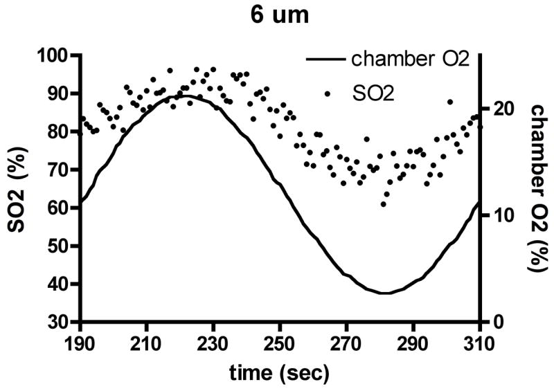
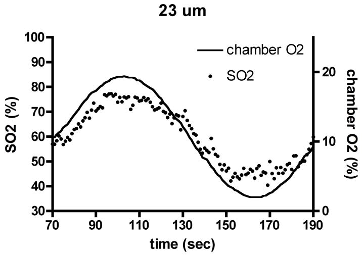
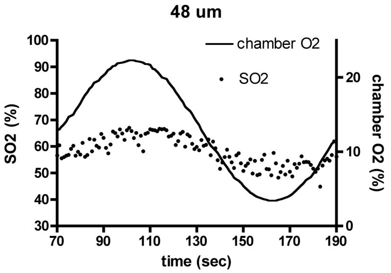
Experimental results for capillary O2 saturation (SO2) changes (dots, left axis) during applied oscillations in muscle surface O2 (lines, right axis) in the absence of local flow regulation. Depths shown: (a) 6 μm, (b) 23 μm, (c) 48 μm. Amplitude and mean of SO2 oscillations decrease with depth into tissue, but phase remains approximately constant.
In what follows, we present a 1D reaction-diffusion equation that models oxygen delivery by capillaries and oxygen diffusion and consumption in muscle tissue. We present an exact periodic solution for the 1D oxygen transport model and show that it generally agrees with experimental data for the case where blood flow is not being regulated. We also present approximate periodic solutions for the low- and high-frequency cases, the latter of which agrees with the solution for pure diffusion. Finally, we discuss the importance of these results for blood-tissue oxygen transport and for future work on local regulation of tissue O2 delivery.
2 Mathematical Model and Exact Solutions
The mathematical model used is specifically tailored to skeletal muscle and the relevant experimental conditions. To reduce the dimensionality of our model, we consider a fixed arterio-venous (A-V) location (‘y’ in Figure 2) in the capillary bed and assume that the distribution of capillary convective O2 supply is approximately homogeneous in the cross-flow direction (‘z’ in Fig. 2). For simplicity, we also assume capillary homogeneity with depth into the tissue (‘x’ in Fig. 2). In effect, the average values of capillary spacing and O2 supply in the z and x directions are being assumed in this model. Therefore, the 1D partial differential equation used in the model could be derived through an averaging process as the zeroth-order approximation to the full 3D equation that includes realistic heterogeneity in z and x. We expect that local deviations from the average properties assumed in the 1D model will lead to local differences in the dynamics of tissue PO2. However, at this stage we are interested only in the average (or bulk) behavior of tissue PO2 as a function of time and depth, and so our 1D model should represent an appropriate approximation.
Figure 2.
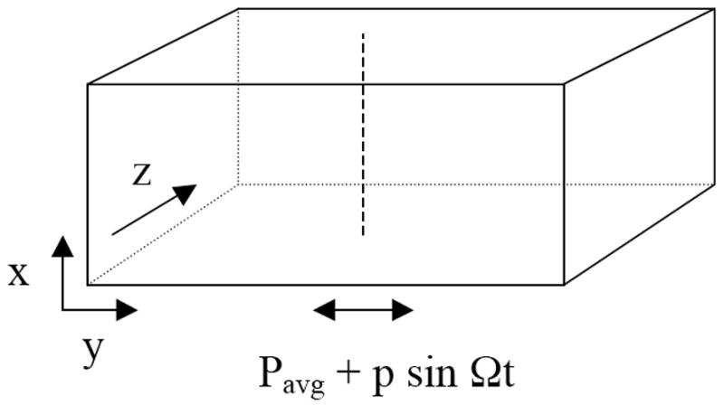
Schematic of three-dimensional experimental situation modeled as one-dimensional problem along dashed vertical line (‘x’ direction). Capillaries and muscle fibers run in ‘y’ direction and oscillating PO2 is applied at lower muscle surface given by x=0.
In the experimental situation being modeled, the oscillating boundary PO2 is such that the tissue PO2 in normal resting muscle remains relatively high. Therefore, neither oxymyoglobin desaturation nor submaximal local O2 consumption is expected. In this case, the role of Mb in facilitating tissue O2 diffusion can be ignored and tissue O2 consumption can be assumed constant. However, we include a PO2-dependent description of the dual role of capillaries as sources and sinks under the given experimental conditions. We use a reference value for average capillary PO2 and assume that for lower local tissue PO2 values the capillary acts as an O2 source, while for higher values it acts as an O2 sink. The coefficient of this term models the combined effects of average capillary density and intravascular O2 transport resistance, with the exact value determined to give physiological values for tissue PO2 at steady state.
Given the above considerations, we use the following time-dependent 1D model for tissue PO2:
| (1) |
where D and α are the tissue O2 diffusion coefficient and solubility, respectively, M0 is the local O2 consumption rate (with units of ml O2/ml tissue/sec), K is a constant that depends on the capillary mass-transfer coefficient and density (and has units of mmHg/sec), and P* is the average capillary PO2. The local concentration of O2 is given by αP, implying that the units of α are ml O2/ml tissue/mmHg.
In equation (1), three effects are included that can change the local tissue PO2 at a given time t. The first of these is diffusion of O2, given by the term D∂2P/∂x2, which occurs in living tissue due to O2 gradients and can serve to increase or decrease P. O2 diffusion would normally occur in all three spatial directions; however, variations in y and z are not included in the model. The second effect included in (1), given by −M0/α, is consumption of O2 by tissue, which is assumed to occur at a constant rate (since P is assumed to remain far above the critical value of about 1mmHg) and acts to decrease P. The third effect included in (1), given by K(1−P/P*), is blood-tissue O2 transfer. This effect is the principal one that is approximated or ‘modeled’ in equation (1), since in reality blood-tissue O2 transfer depends on the local capillary and tissue PO2 distributions. Because we do not wish to consider small-scale details of capillary geometry, spacing, and O2 supply, we use the parameter K to represent the average flux of O2 for a given difference between tissue (P) and capillary (P*) PO2 values.
In order to simplify the analysis of equation (1), we now rearrange it slightly to obtain:
| (2) |
where A=K−M0/α and B=K/P*. This form of the governing equation shows that, in addition to D, there are two constants (assumed to be positive) that determine the dynamics of P: A, which represents the balance between capillary O2 supply and tissue O2 consumption when P=0 (maximum O2 flux into the tissue); and B, which determines how O2 flux into the tissue decreases for P>0.
Equation (2) is an inhomogeneous second-order linear partial differential equation of parabolic type. More specifically, it is a linear 1D reaction-diffusion equation with inhomogeneous term A. For appropriate initial and boundary values, it will have a solution that is well-behaved (i.e., bounded at any finite time and continuous for t>0) and unique [13, 14]. In addition, the full solution P(x,t) to any initial-boundary value problem for (2) can be explicitly obtained using standard methods (algebraic transformation of the equation, separation of variables, Laplace or Fourier transforms; see [15, 16]). As shown below, the typical approach to solving an equation such as (2) is to first solve the steady-state problem. The full equation is then transformed to eliminate the inhomogeneous term and the time-dependent solution is found. Since we will be considering boundary conditions that are periodic in time, the time-dependent solution will have both transient and periodic parts. Here we focus on the time-periodic solution and therefore do not consider the transient solution.
For steady-state conditions, we use boundary conditions for x ≤ 0 and t ≤ 0 that represent PO2 being fixed at Pavg at the surface of the muscle (x=0):
| (3) |
where the second boundary condition is required to eliminate the exponentially growing solution (ebx), which would lead to an unphysical result (infinite PO2) as x → ∞.
Integration of the steady-state form of the partial differential equation (2) then yields the solution:
| (4) |
where . Thus, far from the surface at which its value is set, tissue PO2 is determined by the balance between O2 delivery and consumption inherent in the governing equation. The constant b represents the rate at which the tissue PO2 changes from the value set at the surface (P(x=0)=Pavg) to its natural far-field value (P(x → ∞)=A/B). As the diffusion coefficient D increases, b becomes smaller because the influence of the surface PO2 extends further into the tissue. On the other hand, as the constant B increases, b becomes larger because the effect of capillary O2 delivery to the tissue becomes stronger.
For periodic conditions, we use the following boundary conditions on PO2 for x, t ≥ 0:
| (5) |
The exact periodic solution to (2), assuming all transients have disappeared, is then:
| (6) |
where ω=Ω/B. When no oscillations are imposed at the muscle surface (p=0), we recover the steady-state solution (4). For p > 0, the changes with depth (x > 0) in the amplitude and phase of tissue PO2 will depend on the parameters b and ω. b is a wavenumber (inverse length) scale that is determined by the magnitude of O2 convection relative to O2 diffusion, while ω is the ratio of the forcing frequency to the natural frequency of O2 convection. ω can also be viewed as the ratio of the timescale of O2 convection (1/B) to the forcing period (T=2π/Ω).
For the parameters listed in Table 1, Figure 3 shows the behavior of the exact solution (6). Fig. 3a shows typical behavior of tissue PO2 in time and space, while Figs. 3b and 3c show the dependence of the amplitude and phase of the solutions (6) on normalized depth (ξ= x*b) and ω. At low frequencies (Fig. 3b), the phase of oscillations changes very slowly with depth and attenuation of the oscillation amplitude is essentially independent of frequency. At high frequencies (Fig. 3c), the phase of oscillations changes more rapidly with depth and attenuation increases rapidly with frequency (high-frequency solution below implies amplitude factor of for this case). Note that the behavior of tissue O2 oscillations in the 1D in vivo model (6) does not depend on the O2 consumption parameter A.
Table 1.
Parameters used in 1D O2 transport model.
| Parameter | Value | Reference |
|---|---|---|
| D | 2.41·10−5 cm2/s | Goldman et al., 2004 |
| α | 3.89·10−5 ml O2/ml/mmHg | Goldman et al., 2004 |
| M0 | 1.50·10−4 ml O2/ml/s | Goldman et al., 2004 |
| P* | 48 mmHg | See text |
| K | 30 mmHg/s | See text |
Figure 3.
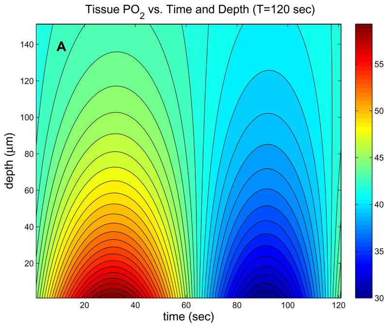


Behavior of exact 1D in vivo solution. (a) Contour plot of tissue PO2 showing dependence on time and depth for period T=120 sec. (b) Contour plots of the amplitude and phase (vs. ω= ΩB and ξ=x*b) showing the low-frequency behavior, which is similar to in vivo experimental observations. (c) Contour plots of the amplitude and phase showing the high-frequency behavior, which is similar to the pure diffusion solution.
3 Approximate Solutions for Low and High Frequencies
Although the exact solution (6) can be evaluated directly, the frequency dependence is more easily understood by examining the limiting cases of low (ω ≪ 1) and high (ω ≫ 1) frequencies. For ω ≪1, we can use a first-order Taylor series to obtain:
| (7) |
With this approximation, we can then show that (6) becomes:
| (8) |
A comparison between the approximation (8) and the exact solution is shown in Fig. 4a. The amplitude and phase of the approximation (8) are both fairly accurate even for ω=1, and become indistinguishable from the exact values for ω<0.1. Since ω ≪1, we have cos(ωbx/2) ≈ 1 and sin(ωbx/2) ≈ 0. Therefore, the cosΩt term is very small and the phase of the imposed PO2 oscillations changes very little with depth into the tissue. This same behavior has been observed experimentally, as shown in Fig. 1. Note that in the limit ω→0 the approximation (8) becomes:
| (9) |
in which there is no phase change with depth.
Figure 4.


Comparison of approximate solutions to exact solution. (a) Approximate solution for ω ≪1. Good agreement with exact solution is seen up to ω=1. (b) Approximate solution for ω ≫1. Agreement with exact solution requires ω ≥10.
For the case ω ≫1, we use a first-order Taylor expansion in 1/ω to obtain:
| (10) |
Using , we approximate (6) as:
| (11) |
The solution (11) has the same steady state as the exact solution (first two terms on right-hand side) and shows the effect of frequency on oscillation amplitude for large ω. In particular, while attenuation was almost independent of frequency for small ω, it now increases with ω in proportion to . The change in oscillation phase with depth also is seen to depend on the quantity . A comparison between the above approximation and the exact solution is shown in Fig. 4b. The amplitude and phase of (11) shown good agreement with the exact values for ω=1 and become highly accurate for ω ≥10. Since ω is large, the decrease in oscillation amplitude with depth will be greater for high frequencies and the phase change with depth will be significant.
The above high-frequency behavior has not been tested for tissues with a functional microcirculation (i.e., local O2 sources/sinks) but, interestingly, it is similar to what would be expected in the absence of microcirculatory transport. In particular, noting that and dropping the first-order 1/(2ω) terms, the solution (11) can be rewritten as:
| (12) |
where . This should be compared to the classical solution for pure diffusion (A=B=0 in (2)) with an oscillating boundary PO2:
| (13) |
The change with depth in the amplitude and phase of the imposed oscillations is identical in (12) and (13), indicating that at high frequencies perfused tissue responds as if it did not have a microvasculature. The above two solutions become even more similar if b is small, i.e., when O2 convection is small compared to O2 diffusion, and become identical for b → 0 (or if Pavg=A/B).
4 Predicted Tissue PO2 Oscillations and Comparison to Pure Diffusion Solution
In the results above, the parameters Pavg, p, and A were not needed to examine the oscillatory part of the solution (6). All other parameters in the model (2)–(6) were fixed with the exception of Ω, which was varied via ω. Some of these fixed parameters are basic physiological quantities that have known values, in particular: the tissue O2 consumption rate (M0), the tissue O2 diffusivity (D), and the tissue O2 solubility (α). We now specify additional parameters needed to predict the actual changes that would be observed experimentally. Based on imposed boundary PO2 oscillations that have been used thus far, we set Pavg=45mmHg and p=15mmHg. P* is chosen to match the average capillary SO2 value halfway between the arteriolar and venular ends, which is necessary because the model does not include variations in the axial or flow direction (‘y’ in Fig. 2). For a different choice of A-V location, the value of P* will need to be adjusted (see below). Given M0, α, and P*, K=30mmH/s is chosen to give A/B≈42mmHg, based on the average tissue PO2 found in experiment-based 3D simulations of capillary-tissue O2 transport in the rat extensor digitorum longus (EDL) muscle [2]. The value of B then becomes K/P*=0.625/s and .
Given the above parameters, we can predict variations in tissue PO2 caused by the imposed oscillations at the muscle surface. The left column in Fig. 5 shows the predictions of our 1D in vivo model for four different depths and three different frequencies. It can be seen that, at the low frequencies being considered experimentally in the Ellis laboratory (periods of ~120s, Fig. 5a), attenuation of the oscillations with depth is large while the phase change with depth is small. Even at slightly higher frequencies (period of 7.5s), attenuation does not increase substantially, implying the low-frequency solution (8) is still valid. Comparing the solutions of the in vivo model to the pure diffusion solutions, we see major qualitative differences in how the amplitude and phase of the imposed oscillations change with depth. For low frequencies, the in vivo model predicts more attenuation of amplitude with depth, while at higher frequencies the amplitudes given by the in vivo and pure diffusion models are comparable since in the in vivo case attenuation is only weakly dependent on frequency. For all frequencies and depths considered, the in vivo model predicts that the phase of tissue PO2 oscillations will be much closer to that of the forcing, i.e., less phase lag.
Figure 5.


Solutions of 1D in vivo model and 1D pure diffusion model for experimental parameters. (a) Results for T=120s and depths of 10, 60, and 150 microns. (b) Results for T=7.5s and depths of 10, 60, and 150 microns. The in vivo model has much higher attenuation and lower phase shift with depth for low frequencies. The phase of the in vivo model becomes more depth-dependent at higher frequencies, but attenuation remains less frequency-dependent than in the pure diffusion model.
By assuming K is a fixed parameter in the 1D in vivo model (representing the maximal rate of blood-tissue O2 transport), we can vary P* (and hence B=K/P*) to predict how oscillations will vary with A-V location. Fig. 6a shows these results for P*=43mmHg. Comparing these results to those in Fig. 5a for P*=48mmHg, it can be seen that the mean of the imposed oscillations decreases more with depth for lower P* (closer to the capillary exit). This is because as P* decreases, A/B decreases, increasing the difference between the mean PO2 imposed at the boundary (Pavg) and the natural far-field mean of tissue PO2 (A/B). Therefore, as the term (Pavg−A/B) e−bx in Eq. 8 decreases with depth it has a greater effect on the overall solution. As P* decreases, there is also an increased exponential decay with depth of both the mean and the oscillation amplitude, due to increasing B. However, this effect is relatively small compared to the changes in Pavg−A/B (see Fig. 6b). These results imply that A-V location will be important to consider when making experimental measurements, as well as when comparing data to theoretical results.
Figure 6.


Dependence of oscillations on P* predicted by 1D in vivo model. (a) tissue PO2 vs. time and depth for T=120s and P*=43mmHg. (b) results for P*=53mmHg and P*=43mmHg, where at each depth the results for the latter case have been shifted up to have the same maximum value as the former. This comparison shows that the mean values of the PO2 oscillations are more sensitive to P* than are the amplitudes.
5 Conclusions
We have presented a simple 1D model of tissue O2 delivery and consumption that predicts how tissue PO2 will vary with time and depth as a result of imposed PO2 oscillations at one surface of an exteriorized skeletal muscle. For the parameters being used experimentally, the predictions of this model are markedly different from what would be expected for pure diffusion. In contrast to the pure diffusion model, the 1D in vivo model implies that with increasing depth there is: i) an exponential change in the mean of tissue PO2, ii) a very rapid decrease in the amplitude of tissue PO2 oscillations, and iii) a very small change in the phase of tissue PO2 oscillations relative to the imposed surface oscillations.
All three of these results have implications for experiments that are currently being conducted in the Ellis laboratory. First, the potential for varying mean tissue PO2 suggests that the imposed surface oscillations should have the same mean as the tissue would normally have (A/B), in order to stimulate flow regulation purely in response to the oscillations themselves rather than the mean. Second, the rapid decay of the imposed oscillations with depth implies that in the EDL muscle only capillaries and parts of the smallest arterioles and venules (i.e., microvessels close to the muscle surface) are being affected, so that the flow response will be due mainly to signals propagated upstream from capillaries. Third, the relatively constant phase of the imposed oscillations implies that all surface capillaries will experience the same time variation in the surrounding PO2. Therefore, the evoked responses in the endothelium of all affected capillaries should be nearly synchronous (though of different magnitudes) and the propagated signals from different capillaries should arrive at upstream locations (arterioles) at nearly the same time. Based on these predicted features, we expect the stimulation protocol to be well suited to determining how changes in capillary SO2 result in compensatory changes in capillary O2 supply (determined by capillary RBC velocity, hematocrit, and inlet SO2).
The 1D in vivo model also predicts that all stimulation periods >30s will lead to essentially the same variation in the mean, amplitude, and phase of tissue PO2 oscillations with respect to depth and phase of the forcing (Fig. 5a). Therefore, observed differences in the flow response to periods in this range will not be due to changes in the spatial distribution of the O2 stimulation, but rather to the inherent frequency dependence of the flow control system. This fact, in combination with such data as the speed of the conducted response, should allow interpretation of observed flow responses in terms of the level of arteriolar control that is involved.
Acknowledgments
The author would like to acknowledge helpful discussions with Dr. Christopher G. Ellis and data provided by Ms. Stephanie Milkovich. This work was supported by grants from the Heart and Stroke Foundation of Ontario (to CGE) and the National Institutes of Health (HL089125).
Footnotes
Publisher's Disclaimer: This is a PDF file of an unedited manuscript that has been accepted for publication. As a service to our customers we are providing this early version of the manuscript. The manuscript will undergo copyediting, typesetting, and review of the resulting proof before it is published in its final citable form. Please note that during the production process errors may be discovered which could affect the content, and all legal disclaimers that apply to the journal pertain.
References
- 1.Beard DA, Schenkman KA, Feigl EO. Myocardial oxygenation in isolated hearts predicted by an anatomically realistic microvascular transport model. Am J Physiol Heart Circ Physiol. 2003;285(5):H1826–36. doi: 10.1152/ajpheart.00380.2003. [DOI] [PubMed] [Google Scholar]
- 2.Goldman D, Bateman RM, Ellis CG. Effect of sepsis on skeletal muscle oxygen consumption and tissue oxygenation: interpreting capillary oxygen transport data using a mathematical model. Am J Physiol Heart Circ Physiol. 2004;287(6):H2535–44. doi: 10.1152/ajpheart.00889.2003. [DOI] [PubMed] [Google Scholar]
- 3.Secomb TW, et al. Analysis of oxygen transport to tumor tissue by microvascular networks. Int J Radiat Oncol Biol Phys. 1993;25(3):481–9. doi: 10.1016/0360-3016(93)90070-c. [DOI] [PubMed] [Google Scholar]
- 4.Ellis C, Milkovich S, Goldman D. Experimental protocol investigating local regulation of oxygen supply in rat skeletal muscle in vivo. Journal of Vascular Research. 2006;43:45. [Google Scholar]
- 5.Milkovich SL, et al. Local regulation of oxygen supply in rat skeletal muscle in vivo: variations in hemodynamic response. FASEB Journal. 2007;21:A481. [Google Scholar]
- 6.Ellsworth ML. Red blood cell-derived ATP as a regulator of skeletal muscle perfusion. Med Sci Sports Exerc. 2004;36(1):35–41. doi: 10.1249/01.MSS.0000106284.80300.B2. [DOI] [PubMed] [Google Scholar]
- 7.Ellis CG, Ellsworth ML, Pittman RN. Determination of red blood cell oxygenation in vivo by dual video densitometric image analysis. Am J Physiol. 1990;258(4 Pt 2):H1216–23. doi: 10.1152/ajpheart.1990.258.4.H1216. [DOI] [PubMed] [Google Scholar]
- 8.Ellis CG, et al. Application of image analysis for evaluation of red blood cell dynamics in capillaries. Microvasc Res. 1992;44(2):214–25. doi: 10.1016/0026-2862(92)90081-y. [DOI] [PubMed] [Google Scholar]
- 9.Japee SA, Ellis CG, Pittman RN. Flow visualization tools for image analysis of capillary networks. Microcirculation. 2004;11(1):39–54. doi: 10.1080/10739680490266171. [DOI] [PubMed] [Google Scholar]
- 10.Japee SA, Pittman RN, Ellis CG. Automated method for tracking individual red blood cells within capillaries to compute velocity and oxygen saturation. Microcirculation. 2005;12(6):507–15. doi: 10.1080/10739680591003341. [DOI] [PubMed] [Google Scholar]
- 11.Japee SA, Pittman RN, Ellis CG. A new video image analysis system to study red blood cell dynamics and oxygenation in capillary networks. Microcirculation. 2005;12(6):489–506. doi: 10.1080/10739680591003332. [DOI] [PubMed] [Google Scholar]
- 12.Batchelor GK. An introduction to fluid dynamics. Cambridge: Cambridge University Press; 1987. pp. 186–193. [Google Scholar]
- 13.Berg PW, McGregor JL. Elementary partial differential equations. San Francisco: Holden-Day; 1966. [Google Scholar]
- 14.Britton NF. Reaction-diffusion equations and their applications to biology. London: Academic Press; 1986. [Google Scholar]
- 15.Farlow SJ. Partial differential equations for scientists and engineers. New York: Dover; 1993. [Google Scholar]
- 16.Pinsky MA. Partial differential equations and boundary-value problems with applications. New York: McGraw-Hill; 1991. [Google Scholar]