Space–time clustering of case–control data with residential histories: insights into empirical induction periods, age-specific susceptibility, and calendar year-specific effects

Abstract

Our research group recently developed Q-statistics for evaluating space–time clustering in case–control studies with residential histories. This technique relies on time-dependent nearest-neighbor relationships to examine clustering at any moment in the life-course of the residential histories of cases relative to that of controls. In addition, in place of the widely used null hypothesis of spatial randomness, each individual's probability of being a case is based instead on his/her risk factors and covariates. In this paper, we extend this approach to illustrate how alternative temporal orientations (e.g., years prior to diagnosis/recruitment, participant's age, and calendar year) influence a spatial clustering pattern. These temporal orientations are valuable for shedding light on the duration of time between clustering and subsequent disease development (known as the empirical induction period), and for revealing age-specific susceptibility windows and calendar year-specific effects. An ongoing population-based bladder cancer case–control study is used to demonstrate this approach. Data collection is currently incomplete and therefore no inferences should be drawn; we analyze these data to demonstrate these novel methods. Maps of space–time clustering of bladder cancer cases are presented using different temporal orientations while accounting for covariates and known risk factors. This systematic approach for evaluating space–time clustering has the potential to generate novel hypotheses about environmental risk factors and provides insights into empirical induction periods, age-specific susceptibility, and calendar year-specific effects.

1 Introduction

Pattern recognition plays an important role in the analysis of geographic distributions of disease by providing an objective basis for evaluating whether pattern on a map is likely to be explained by chance (Waller and Jacquez 1995). Dozens of approaches are available for quantifying pattern on disease maps (e.g., Besag and Newell 1991; Cuzick and Edwards 1990; Kulldorff and Nagarwalla 1995; Kulldorff et al. 2006; Tango and Takahashi 2005; Turnbull et al. 1990; Waller and Turnbull 1993; Waller et al. 1995); however, most of these tests were developed for spatially static datasets and therefore rely on assumptions that individuals are immobile, and that the latency between causative exposures and health events (e.g., diagnosis and death) is negligible (Jacquez 2004). In most analyses, only place of residence at time of diagnosis or time of death is used to record the locations of health events.

When analyzing chronic diseases such as cancer, causative exposures may occur many years prior to disease diagnosis. The duration of time from initial etiologic action of a causative exposure to disease detection has been called the empirical induction period (Rothman 1981). During this empirical induction period individuals may move from one place of residence to another. Failure to account for residential mobility, therefore, can make detecting clustering of cases in relation to the spatial distribution of their causative exposures difficult or even impossible. Recent studies demonstrate that results obtained using methods that assume static spatial point distributions at time of diagnosis or death fail to capture the full magnitude of the spatial pattern and can lead to erroneous conclusions regarding the timing, existence, extent, and locations of disease clusters (Jacquez et al. 2005; Sabel et al. 2003).

A priori hypotheses concerning the timing of clustering often do not exist. In these situations, health researchers may wish to investigate whether clustering at any point in time is associated with development of disease. Furthermore, without clear intuition regarding the appropriate temporal model, researchers might want to consider multiple temporal orientations: e.g., participants' age, calendar year, and years prior to diagnosis/recruitment. The time-geographies may differ when using these three orientations. For example, if residences are mapped based on where participants lived when they were born, participants will be mapped near one another if they were born in the same geographic area, even if born in different calendar years. Similarly, if residences are mapped based on where participants lived in a given calendar year (e.g., 1975), individuals of different ages will be mapped near one another. As another example, if residences are mapped based on where participants lived 10 years prior to diagnosis/recruitment, individuals of different ages and individuals diagnosed in different calendar years will be mapped near one another. These three temporal orientations can result in unique time-geographies that reveal different aspects of spatial pattern reflecting underlying associations between disease risk and the timing of events over a life-course. Therefore, factoring in human mobility and multiple temporal orientations may be valuable for investigating spatial patterns of chronic diseases with long empirical induction periods.

To characterize human mobility, Hagerstrand (1970) proposes constructs for representing the space–time paths formed as individuals move throughout their days, now known as geospatial life-lines (Sinha and Mark 2005). Several recent efforts have applied this concept of geospatial life-lines and furthered our ability to identify space–time disease clusters (Han et al. 2004, 2005; Ozonoff et al. 2005; Paulu et al. 2002; Sinha and Mark 2005; Vieira et al. 2005). All of these approaches, however, analyze static spatial point distributions at a few snapshots in time, and therefore do not fully account for human mobility. They fail to account for underlying temporal changes in place of residence, and they do not provide measures of spatial pattern between time slices. These methods, therefore, do not provide a complete and detailed analysis of clustering at any moment over a life-course.

Individual mobility is poorly characterized in cancer cluster analyses, in part, because of dependence on traditional geographic information systems (GIS). Traditional GIS are based on spatial data structures–the “what, where” dyad that inadequately displays changes through time. These spatial data structures cannot readily deal with space–time georeferencing or space–time queries (Jacquez 2000), and instead are best suited for generating “snapshots” in time of static systems (Hornsby and Egenhofer 2000). Recent advances in Space–Time Information Systems (STIS) technology, however, enable characterization of the “what, where, when” triad needed for effective representation of data used to analyze health outcomes (Avruskin et al. 2004; Meliker et al. 2005). STIS rely on space–time data structures, thereby enabling powerful epidemiological queries that are not possible through “space only” GIS. STIS technology allows a user to observe and quantify how geographies change with time. This technology is necessary for implementing the mathematical and statistical algorithms underlying our Q-statistic, and is required to assess space–time clustering in case–control data.

Our research team recently developed global, local, and focused versions of Q-statistics for evaluating space–time clustering in residential histories using case–control data (Jacquez et al. 2005). This approach is based on a space–time representation that is consistent with Hagerstrand's notion of space–time paths. The Q-statistics utilize the residential history of participants represented as a life-line, and thus evaluate local, global, and focused clustering at any moment in the life-course of the residential histories of cases relative to the residential histories of controls. One of the benefits of the different versions of the Q-statistics is their ability to quantify what is happening at the local, spatial, and temporal scales that is of relevance to individuals, while also providing global statistics for evaluating aggregations of cases.

The Q-statistics also have been shown to detect clustering after accounting for known risk factors (e.g., smoking) and covariates (such as age at time of interview, race, and sex) (Jacquez et al. 2006). By using “neutral models” to specify spatial null hypotheses, each individual's probability of being a case based on his/her known risk factors and covariates is incorporated into the assignment of case–control identifiers (Goovaerts and Jacquez 2004). The resulting null hypothesis then is not one of spatial independence (the widely used but often inappropriate null hypothesis of many cluster tests); rather, it accounts for the geographic distribution of covariates and known risk factors. Thus any observed case clustering cannot be attributed to geographic variation in the modeled risk factors and covariates, and instead may be due to geographic pattern in some other, perhaps unknown, risk factor.

The aim of this paper is to illustrate how alternative temporal orientations influence space–time clustering results in an ongoing bladder cancer case–control study. Q-statistics and spatial null hypotheses that account for risk factors and covariates are applied to investigate spatial pattern in residential histories using calendar year, participants' age, and years prior to diagnosis/recruitment as alternative temporal orientations.

2 Methods

In this section Q-statistics and methods for constructing spatial null hypotheses that account for risk factors and covariates are briefly reviewed. This methodological approach then is extended to calculate global and local clusters using alternative temporal orientations. Next, a bladder cancer case–control study in southeastern Michigan is described, followed by an application of these methods to this dataset to illustrate the approach.

2.1 Q-statistics and spatial null hypotheses

Jacquez et al. (2005, 2006) develop global, local, and focused tests for case–control clustering of residential histories that account for covariates and other risk factors. Readers unfamiliar with Q-statistics may wish to refer to the original works. Q-statistics rely on a matrix representation that describes how spatial nearest neighbor relationships change through time. Versions of the Q-statistics that are applied in this paper are described below.

To identify the location and timing of significant clustering, the following spatially and temporally local case–control cluster statistic is used:

$$Q_{i,k,t}=c_i\sum _{j=1}^N{\eta }_{i,j,k,t}{c}_j.$$ (1)

This quantity is the count, at time t, of the number of k nearest neighbors of case i that are cases, and not controls. Individuals i and j have case–control identifiers, c_i and c_j defined to be 1 if and only if a case, and 0 otherwise. N is the total number of participants (cases and controls) in a study. The term η_i,j,k,t is a binary spatial proximity metric that is 1 when participant j is a k nearest neighbor at time t of participant i; otherwise it is 0. Since a given individual i may have k unique nearest neighbors, the Q_i,k,t statistic is in the range 0…k. When i is a control, Q_i,k,t = 0. When i is a case, low values indicate cluster avoidance (e.g., a case surrounded by controls), and large values indicate a cluster of cases. When Q_i,k,t = k, at time t all of the k nearest neighbors of case i are cases. This statistic is recalculated for each participant every time there is a change in residence. Therefore, Eq. 1 reports a value for each residence at each and every time–geography of the residential histories.

To determine if global clustering is present, the following equations are needed:

$$Q_{i,k,{\omega }_o}=c_i\sum _{j=1}^N{\eta }_{i,j,k,t_{\text{o}}}{c}_j{\omega }_o,$$ (2)

$$Q_{k,{\omega }_o}=\sum _{i=1}^N{Q}_{i,k,{\omega }_o,}$$ (3)

$$Q_k^{\omega }=\sum _{o=0}^{T-1}{Q}_{k,{\omega }_o}.$$ (4)

Equation 2 is similar to Eq. 1, only this local statistic is duration-weighted, indicated by ω_o, which refers to the duration of time spent at a residence; residences of longer duration are given greater importance in this statistic. Equation 3 is a global version of this statistic and reports if clustering occurs throughout the entire area at a particular moment in time. It is calculated by summing Eq. 2 all cases at that moment in time. Equation 4, then, gives a measure of global case clustering of residential histories throughout the study area and over the entire study time period. It is calculated by summing Eq. 3, over all T + 1 time points. This statistic indicates whether there is global clustering of residential histories when all of the residential histories over the entire study period are considered simultaneously. It is a measure of the persistence of global clustering and is large when case clustering persists through time.

In the absence of knowledge of covariates and other risk factors, simple randomization may be used when evaluating the statistical significance of the above statistics. This is accomplished by holding the location histories for the cases and controls constant, followed by permuting the case–control identifiers at random over the residential histories. This corresponds to a null hypothesis where the probability of an individual being declared a case (c_i = 1) is proportional to the number of cases in the data set, or

$$p\left(c_i=1|H_{0,I}\right)=\frac{n_1}{n_0+n_1},$$ (5)

where n₁ is the number of cases and n₀ is the number of controls, and this null hypothesis assumes that the risk of being declared a case is the same over all of the N case and controls. When covariates and risk factors are quantified, one may wish to incorporate that information into the null hypothesis. Any case-clustering that is found then will be above and beyond the modeled risk factors and covariates, and thus will indicate the possible presence of risk sources beyond those specified under this null hypothesis.

In order to provide a more realistic null hypothesis, the probability of being declared a case can be calculated as a function of covariates and risk factors. This is accomplished using logistic regression. Let x denote the vector of covariates and risk factors. Further, let p=Pr(c=1|x) denote the response probability to be modeled, which is the probability of person i being a case. The linear logistic model then is

$$\text{logit}\left(p\right)=\text{log}\left[p/\left(1-p\right)\right]=\alpha +\beta \prime \text{x}$$ (6)

and the equation for predicting the probability of being a case given the vector of covariates and risk factors for the ith individual is

$$\widehat{p}(c_i=1|{\text{x}}_i)=\frac{{\text{e}}^{\alpha +\beta \prime x_i}}{1+{\text{e}}^{\alpha +\beta \prime x_i}}.$$ (7)

Here the logit function is the natural logarithm of the odds, α is the intercept parameter, and β is the vector of regression (slope) coefficients. One then fits the regression model to the vector of covariates and risk factors to calculate the intercept and slope parameters. This estimated equation then is used to calculate, for each individual, the probability of being a case given that individual's known covariates and risk factors.

Approximate randomization is used to evaluate the probability of a given Q-statistic under the null hypothesis that the likelihood of being a case is a function of the covariates and risk factors specified in Eq. 7. Evaluating the reference distribution for a given Q-statistic involves the following steps:

• Step 1: Calculate statistic (Q*) for the observed data.

• Step 2: Permute the case–control identifier c_i over the residential histories of the participants in a manner consistent with the desired null hypothesis, and conditioned on the observed number of cases. Assume we have n_a cases, N participants and that P_i is the probability of the ith participant being a case. Notice that the P_i is provided by the logistic equation.

• Step 2.1: Rescale the P_i as follows: $P_i^{\prime }=P_i/{\sum }_{j=1}^N{P}_j.$

• Step 2.2: Map the P_i′ to the interval [0…1]. For example, assume we have N = 2 participants, n_a = 1 case and that P₁ = 0.7 and P₂ = 0.8. P₁′ then maps to the interval [0…0.7/1.5) and P₂′ maps to the interval [0.7/1.5…1.5/1.5).

• Step 2.3: Allocate a case by drawing a uniform random number from the range [0…1). Set the case identifier equal to 1 (c_i = 1) where i is the identifier corresponding to the study participant whose interval for P_i′ contains the random number.

• Step 2.4: Rescale as shown in Step 2.1 but not including the probability for the participant whose case identifier was assigned in Step 2.3.

• Step 2.5: Repeat Steps 2.2–2.4 until all of the n_a case identifiers are assigned.

• Step 2.6: Set the remaining N–n_a case identifiers to 0, these are the controls.

Notice Steps 2.1–2.6 result in 1 realization of the distribution of case–control identifiers.

• Step 3: Calculate Q for the realization from Step 2.

• Step 4: Repeat Steps 2–3 a specified number of times (e.g., 999) accumulating the reference distribution of Q.

• Step 5: Compare Q* to this reference distribution to evaluate the statistical probability of observing Q* under the null hypothesis that accounts for the known risk factors and covariates.

2.2 Temporal orientations

Q-statistics are appropriate for data that contain standard units of time, such as years, months, days, hours, minutes, and seconds. When calculating the duration of time spent at each residence, however, different temporal orientations may be useful to consider: reference to age (i.e., years since birth), reference to diagnosis/recruitment (i.e., years prior to diagnosis/recruitment), or reference to calendar year (i.e., years between two dates on a calendar). Results obtained from using these three temporal orientations are compared in the ensuing analyses.

2.3 Data

A population-based bladder cancer case–control study is underway in southeastern Michigan. Cases diagnosed in the years 2000–2004 and living in Genesee, Huron, Ingham, Jackson, Lapeer, Livingston, Oakland, Sanilac, Shiawassee, Tuscola, and Washtenaw counties are being recruited from the Michigan State Cancer Registry (Fig. 1). Controls are being frequency matched to cases by age (±5 years), race, and gender, and are being recruited using a random digit dialing procedure from an age-weighted list. At this stage of recruitment, controls are not adequately matched; therefore, age, race, and gender are adjusted for in the subsequent analyses. To be eligible for inclusion in the study, participants must have lived in the 11-county study area for at least the past 5 years and have no prior history of cancer (with the exception of non-melanoma skin cancer). Participants are offered a modest financial incentive and research is approved by the University of Michigan IRB-Health Committee. The data analyzed here are from 219 cases and 437 controls (Table 1).

Fig. 1.

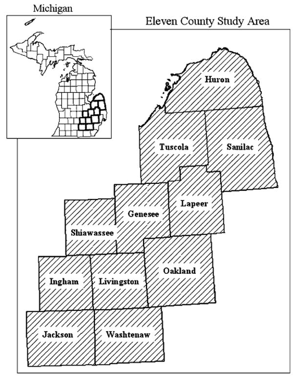
Eleven-county study area in southeastern Michigan

Table 1.

Demographic and descriptive characteristics of 219 cases and 437 controls

	Cases (%)	Controls (%)
Age (years)
30–39	1	2
40–49	6	8
50–59	20	9
60–69	33	48
≥70	40	32
Gender
Male	77	87
Female	23	13
Race
Caucasian/white	95	92
African American/black	1	3
Asian/Asian American	1	2
American Indian or Alaskan native	3	3
Education
≤ High school	39	25
Some post-high school	30	26
College graduate	19	22
Post-graduate education	12	27
Total number of residences	1,624	3,434
Percent of person-years in study area	66	63

Percentages do not always equal 100% due to rounding

Participants completed a written questionnaire describing their residential mobility, providing the years moved in and out of each residence and its exact street address. If exact address is not known, closest cross-streets are provided. On average, 66 years of residential history were collected for each participant, with a mean duration of 8 years (median 6 years) at each residence. Participants changed residences eight times, on average. Cases averaged 1 year longer at each residence compared with controls. Each residence in the study area was geocoded and assigned a geographic coordinate in ArcGIS (Version 9.0; ESRI, Redlands, CA, USA); residences outside the study area were not geocoded. Approximately 66% of cases' person-years and 63% of controls' person-years were spent in the study area. Of the residences within the study area, 88% were automatically geocoded or interactively geocoded with minor operator assistance. The unmatched addresses were manually geocoded using self-reports of cross-streets with the assistance of internet mapping services (6%); if cross-streets were not provided or could not be identified, residence was matched to town centroid (6%).

2.4 Statistical analyses

Global and local Q-statistics, unadjusted and statistically adjusted, were calculated to examine space–time clustering of residential histories of bladder cancer cases and controls using the following three temporal orientations: age, calendar year, and years prior to diagnosis/recruitment.

Q-statistics were computed using STIS^™ (Version 1.2; TerraSeer Inc., Crystal Lake, IL, USA) and the number of nearest neighbors was allowed to vary from k = 6 to 10, to explore how sensitive cluster location and strength is to the number of nearest neighbors. Concordance of results across different levels of k is used to reach conclusions regarding clustering. The global Q-statistic was duration-weighted (Eq. 4) and used to assess global clustering of residential histories when all of the residential histories over the entire study period are considered simultaneously. The local Q-statistic (Eq. 1) is used to assess clustering at each residence, and it was recalculated every time a participant moved to a different residence. Local clustering that persisted in the same area for five consecutive years across the different levels of k is reported.

To account for covariates and risk factors in the Q-statistics, an unconditional logistic regression analysis was executed using “proc logistic” in Statistical Analysis System^® (Version 8.0; SAS Institute Inc., Cary, NC). The following covariates and risk factors were included in the logistic regression model: age at time of interview, sex, race, level of education, and average number of cigarettes smoked daily. These parameters have been summarized as being significant for bladder cancer and are commonly adjusted for in epidemiologic investigations of bladder cancer (Silverman et al. 1996). The parameter estimates of the model were used to estimate a probability of being a case (Eq. 7) for each participant and included in the statistically adjusted analyses of the Q-statistics in STIS^™.

3 Results

Since the study is still ongoing, results are presented only to demonstrate the novel space–time clustering approach. In these preliminary analyses, residential histories of cases cluster over the entire study period when the time–geography is based on calendar years (Table 2). The clustering remains significant under unadjusted (spatial randomness) and statistically adjusted (smoking, education, and covariates) spatial null hypotheses, regardless of the number of nearest neighbors selected (k ranged from 6 to 10). Using a time–geography of residential locations during years prior to diagnosis/recruitment, clustering is significant in the unadjusted analyses, but no longer significant once adjusted for smoking, education, age at time of interview, race, and sex. Again, these results are consistent regardless of the number of nearest neighbors selected. The third time–geography of residential locations during different ages is not significant in unadjusted or adjusted analyses, and is consistent for k from 6 to 10.

Table 2.

The value of global Q-statistics for clustering under three temporal orientations: participants' age, years prior to diagnosis/recruitment, and calendar year

Age of participants				Years prior to diagnosis/recruitment			Calendar year
k	Qk	p(Qk |ind)	p(Qk |cov)	Qk	p(Qk |ind)	p(Qk |cov)	Qk	p(Qk |ind)	p(Qk |cov)
6	0.75	0.20	0.42	0.84	0.032	0.12	1.03	0.001	0.004
7	0.87	0.23	0.43	0.98	0.028	0.13	1.20	0.001	0.003
8	0.99	0.17	0.42	1.12	0.023	0.09	1.37	0.001	0.004
9	1.12	0.16	0.35	1.26	0.034	0.11	1.54	0.001	0.003
10	1.25	0.16	0.41	1.40	0.025	0.12	1.70	0.001	0.004

Unadjusted and statistically adjusted results. Nearest neighbors considered (k = 6–10). Q_k is the value of the global statistic for evaluating clustering of residential histories of cases over the entire study period and study area; p(Q_k |ind) the probability of Q_k under the null hypothesis of spatial independence; p(Q_k |cov) is the probability of Q_k adjusted for smoking, age at time of interview, sex, education, and race

Even though global clustering over the entire study period is significant for only one temporal orientation, local clustering could still be significant in parts of the study area over shorter periods of time. In maps displaying residential locations during different calendar years, the unadjusted analyses reveal persistent clustering for 5 years or longer in Oakland County, from 1960s to 1990s, and in Genesee, Ingham, and Jackson Counties in 1990s. After statistical adjustment, clustering remains in Oakland County in 1960s, 1980s, and 1990s, and in Genesee and Ingham counties in 1990s. Figure 2 shows snapshots for 1960 and 1995 from the continuous time–geography generated in STIS^™. Cases that are the centers of significant clusters are highlighted. This figure displays statistically adjusted clusters in Jackson County in 1995; however, these clusters are transient and do not last for 5 years for any of the levels of k. Also note a few clusters that are significant in the unadjusted analyses, but no longer significant after statistical adjustment.

Fig. 2.

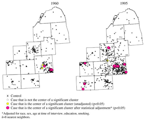
Local clusters of residential histories for different calendar years. Snapshots of continuous animation from STIS. k = 8 nearest neighbors. a 1960. b 1995

The unadjusted analyses revealed persistent clustering in Oakland County in the 10 years prior to diagnosis/recruitment on maps displaying residential locations during years prior to diagnosis/recruitment. No clustering persists at any other time prior to diagnosis/recruitment (Fig. 3). After statistical adjustment, clustering persists in Oakland County and also appears in Ingham County in the 10 years prior to diagnosis. In Fig. 3, the cluster depicted in Jackson County at 5 years prior to diagnosis is transitory.

Fig. 3.

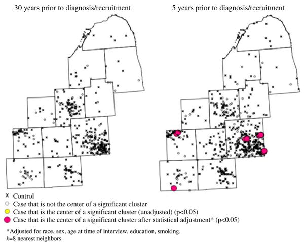
Local clusters of residential histories for time-geographies representing years prior to diagnosis/recruitment. Snapshots of continuous animation from STIS. k = 8 nearest neighbors. a 30 years prior to diagnosis/recruitment. b 5 years prior to diagnosis/recruitment

On maps using the third temporal orientation, participants' age, persistent clustering is observed only along the border of Lapeer and Tuscola Counties when participants were in their late 40s. This cluster remains in unadjusted and adjusted analyses (Fig. 4). Clusters do not appear during other ages. The cluster in Oakland County seen in Fig. 4 is ephemeral.

Fig. 4.

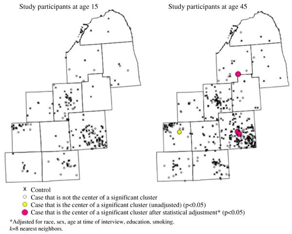
Local clusters of residential histories for time-geographies of participants' ages. Snapshots of continuous animation from STIS. k = 8 nearest neighbors. a Study participants at age 15 years. b Study participants at age 45 years

4 Discussion

The bladder cancer case–control study from which this dataset originated is still in the data collection phase. Therefore, we cannot draw any inferences from the analysis of these data, and have used them only to illustrate how space–time clustering is dependent on the temporal orientation of data. This study is only preliminary and these analyses will be rigorously revisited when data collection is complete, at which time factors potentially responsible for the clusters will be investigated. However, we provide the following discussion to depict how to interpret output from these novel Q-statistics.

In these preliminary analyses, global clustering (after statistical adjustment) is only significant in time-geographies of residential histories at different calendar years. Local clustering, however, is observed with all three temporal orientations in different regions of the study area for durations of at least 5 years. Local clusters are observed in Oakland County in 1960s, 1980s, 1990s, and up to 10 years prior to diagnosis/recruitment. Clusters also are observed in Genesee and Ingham Counties in 1990s and along the border of Lapeer and Tuscola Counties when participants were in their late 40s.

The presence of these clusters implicitly implies underlying risk factors during the aforementioned periods of time. Possible risk factors include industrial pollution, environmental contamination, occupational exposures, diet, and ethnic origin/genetic composition, among others. The multistep model of carcinogenesis suggests that risk factor(s) causing a continuous accumulation of genetic lesions are necessary for cancer genesis (Hahn et al. 1999; Vogelestien and Kinzler 1993). Working under the guidance of this model, exposure to risk factor(s) in 1960s and 1980s conceivably is responsible for early genetic mutations that later resulted in bladder cancer for some individuals. Based on the pattern of the clustering, these risk factor(s) are likely present in Oakland County during the 1960s and 1980s, but not during the 1950s or 1970s. If these results remain in the final analyses, possible risk factors that exhibit a similar spatio-temporal pattern and etiological relevance will be explored, such as different sources and types of industrial pollutants in Oakland County.

Clustering is more pervasive in the more urban parts of the study area in 1990s, which also was when participants were within 10 years of being diagnosed or recruited into the study. Hence the clustering pattern in 1995 (Fig. 2) looks very similar to that seen 5 years prior to diagnosis/recruitment (Fig. 3). This correlation occurs because cases have been diagnosed over a relatively short time window (5 years). The longer the diagnosis period, the less correlation there will be between these two temporal orientations. The similar patterns portrayed in Figs. 2 and 3 may suggest the presence of risk factor(s) responsible for late-stage genetic lesions that elicit bladder carcinogenesis within an empirical induction period of no more than 10 years. Urban risk factor(s) of etiological relevance will be explored if these results are confirmed in the final analyses.

A cluster also is observed for individuals in their late 40s, suggesting a potential age range of susceptibility or vulnerability to bladder carcinogenesis. Any risk factor(s) responsible for this cluster must have been present for many years because the individuals in this cluster, while being of similar age, were in this region during different calendar years. Considering that the global Q-statistic is not significant for time–geographies based on participants' age, and the extent of multiple testing (discussed in more detail below), this cluster is not likely to generate insights of note.

The results reported here clearly indicate the importance of considering multiple temporal orientations when conducting cluster investigations because while one orientation may reveal significant clustering, other temporal orientations may not. Thus, a potential cluster could be missed if several temporal orientations are not explored. This is an important finding because only one temporal orientation is considered in most clustering analyses (Han et al. 2004; Ozonoff et al. 2005; Sinha and Mark 2005).

In terms of disease etiology, different temporal orientations may provide insights into different aspects of a disease process. Rothman (1981) considers empirical induction periods in which specific exposures ultimately lead to full-blown disease. The exposures in isolation may not be a sufficient cause of disease onset; rather, a combination of exposures may be required. The question then arises as to how one might identify the time span over which this suite of constituent exposures occurred. By considering different temporal orientations, an analyst can evaluate alternative hypotheses regarding the timing of exposures. For example, a specific sub-population might have experienced an ephemeral exposure sufficiently damaging to lead directly to disease in many of the exposed individuals, such as occurred in Nagasaki and Hiroshima. In these instances one might use a temporal orientation referenced relative to this known exposure event. Alternatively, one might hypothesize times in a life-course when individuals are thought to be biologically vulnerable to a given exposure, suggesting the use of an age-referenced temporal orientation. Ideally, the selection of the temporal orientation to use in an analysis will be driven by hypotheses regarding specific mechanisms of disease causation. In situations where a reasonable hypothesis is not available, as often is the case, exploratory analyses such as those illustrated in this paper may provide valuable information.

Q-statistics represent a significant methodological advance that enables assessment of the time lag between exposure and diagnosis that is the hallmark of disease processes. By modeling residential histories as a series of connected locations that changes through time, Q-statistics facilitate the ability to: (1) track time spent at different residences, (2) track the changing space–time geometry of the residential histories of a study population, (3) incorporate knowledge of individual-level risk factors and covariates into cluster statistics, and (4) examine how clustering changes under alternative temporal orientations.

Despite these advances, this approach has several limitations. In common with other clustering studies, individuals are mapped only at their home address even though they spend time away from home (e.g., at work, relatives' homes). In addition, the choice of the number of k nearest neighbors is subjective. In this paper k varies from 6 to 10, and concordance of results across different levels of k was used to reach conclusions regarding clustering. The metrics do not need to be nearest neighbor relationships in order for the Q-statistics to work; however, nearest neighbor relationships are invariant under changing population densities, unlike geographic distance and adjacency measures. There also is some evidence that nearest-neighbor metrics are more powerful than distance- and adjacency-based measures (Jacquez 1996). When exploring multiple values of k, however, implications of multiple testing need to be considered. Since this work is exploratory and for hypothesis generation, we use a p = 0.05; this choice ultimately lies with each individual researcher.

Q-statistics are appropriate in case–control studies where participants are recruited in a population-based manner, and no geographic bias is introduced into the sampling frame. Generally, Q-statistics require that time moves in a linear fashion, and that units of time have the same meaning, regardless of when they occur. For example, even though years may “fly by” as people get older, each year of life represents the same duration of time in the Q-statistics. It is possible that given a viable hypothesis about the temporal dynamics of a disease's progression, one may wish to place greater emphasis on years that fall during critical periods of development using a pre-specified temporal orientation. Our research group has begun to consider means of incorporating such a priori temporal hypotheses using estimates of exposure windows and disease latency periods in the Q-statistics, although more work is needed in this area (Jacquez et al. 2005; Jacquez and Meliker, in press). In addition, future research also needs to address the use of time-varying risk factors in the statistical adjustment procedure. Methods for factoring duration of exposure to risk factors (e.g., smoking) into the statistical adjustment, and evaluating interactions between risk factors and clustering are areas of high research priority.

5 Conclusions

The approach presented here is ideally suited to exploratory investigations of space–time clustering in situations where strong a priori hypotheses about the timing of clustering do not exist. Inappropriate assumptions about the length of an empirical induction period can result in non-differential misclassification and bias results toward the null (Rothman 1981). Therefore, repeated clustering tests, such as those presented here, can be used to minimize such misclassification, identify significant spatial clustering at any moment throughout a life-course, and provide estimates of an empirical induction period, age-specific susceptibility windows, and calendar year-specific effects. This approach is suitable for case–control studies with residential histories that contain no geographic bias in case–control selection. The ability of the local tests to quantify pockets of cases in space and time, while accounting for known risk factors and covariates, is of great value for hypothesis generation. Applying the Q-statistics to examine clustering in several temporal orientations has the potential to furnish insights about factors responsible for clustering, and for shedding light on the temporal relationship between those factors and disease.

6 Statement of potential conflict of interest

The authors work at BioMedware Inc., Ann Arbor, MI, the company that is developing the STIS^™ software.

References

- Avruskin GA, Jacquez GM, Meliker JR, Slotnick MJ, Kaufmann AM, Nriagu JO. Visualization and exploratory analysis of epidemiologic data using a novel space time information system. Int J Health Geogr. 2004;3:26. doi: 10.1186/1476-072X-3-26. [DOI] [PMC free article] [PubMed] [Google Scholar]
- Besag J, Newell J. The detection of clusters in rare diseases. J R Stat Soc A Stat. 1991;154:143–155. [Google Scholar]
- Cuzick J, Edwards R. Spatial clustering for inhomogeneous populations. J R Stat Soc B Methodol. 1990;52:73–104. [Google Scholar]
- Goovaerts P, Jacquez GM. Accounting for regional background and population size in the detection of spatial clusters and outliers using geostatistical filtering and spatial neutral models: the case of lung cancer in Long Island, New York. Int J Health Geogr. 2004;3:14. doi: 10.1186/1476-072X-3-14. [DOI] [PMC free article] [PubMed] [Google Scholar]
- Hagerstrand T. What about people in regional science? Pap Reg Sci Assoc. 1970;24:7–21. [Google Scholar]
- Hahn WC, Counter CM, Lundberg AS, Beijersbergen RL, Brooks MW, Weinberg RA. Creation of human tumor cells with defined genetic elements. Nature. 1999;400:464–468. doi: 10.1038/22780. [DOI] [PubMed] [Google Scholar]
- Han D, Rogerson PA, Nie J, Bonner MR, Vena JE, Vito D, Muti P, Trevisan M, Edge SB, Freudenheim JL. Geographic clustering of residence in early life and subsequent risk of breast cancer (United States) Cancer Cause Control. 2004;15:921–929. doi: 10.1007/s10552-004-1675-y. [DOI] [PubMed] [Google Scholar]
- Han D, Rogerson PA, Bonner MR, Nie J, Vena JE, Muti P, Trevisan M, Freudenheim JL. Assessing spatio-temporal variability of risk surfaces using residential history data in a case control study of breast cancer. Int J Health Geogr. 2005;4:9. doi: 10.1186/1476-072X-4-9. [DOI] [PMC free article] [PubMed] [Google Scholar]
- Hornsby K, Egenhofer M. Identity-based change: a foundation for spatio-temporal knowledge representation. Int J Geogr Inf Sci. 2000;14:207–224. [Google Scholar]
- Jacquez GM. Disease cluster statistics for imprecise space–time locations. Stat Med. 1996;15:873–885. doi: 10.1002/(sici)1097-0258(19960415)15:7/9<873::aid-sim256>3.0.co;2-u. [DOI] [PubMed] [Google Scholar]
- Jacquez GM. Spatial analysis in epidemiology: nascent science or a failure of GIS? J Geogr Syst. 2000;2:91–97. [Google Scholar]
- Jacquez GM. Current practices in the spatial analysis of cancer: flies in the ointment. Int J Health Geogr. 2004;3:22. doi: 10.1186/1476-072X-3-22. [DOI] [PMC free article] [PubMed] [Google Scholar]
- Jacquez GM, Kaufmann A, Meliker J, Goovaerts P, AvRuskin G, Nriagu J. Global, local and focused geographic clustering for case–control data with residential histories. Environ Health. 2005;4:4. doi: 10.1186/1476-069X-4-4. [DOI] [PMC free article] [PubMed] [Google Scholar]
- Jacquez GM, Meliker JR, AvRuskin GA, Goovaerts P, Kaufmann A, Wilson M, Nriagu J. Case–control geographic clustering for residential histories accounting for risk factors and covariates. Int J Health Geogr. 2006;5:32. doi: 10.1186/1476-072X-5-32. [DOI] [PMC free article] [PubMed] [Google Scholar]
- Jacquez GM, Meliker JR. Case–control clustering for mobile populations. In: Fotheringham S, Rogerson P, editors. Handbook of spatial analysis. Sage Publications; Beverley Hills, CA: 2007. (in press) [Google Scholar]
- Kulldorff M, Nagarwalla N. Spatial disease clusters: detection and inference. Stat Med. 1995;14:799–810. doi: 10.1002/sim.4780140809. [DOI] [PubMed] [Google Scholar]
- Kulldorff M, Huang L, Pickle L, Duczmal L. An elliptic spatial scan statistic. Stat Med. 2006 doi: 10.1002/sim.2490. [DOI] [PubMed] [Google Scholar]
- Meliker JR, Slotnick MJ, AvRuskin GA, Kaufmann A, Jacquez GM, Nriagu JO. Improving exposure assessment in environmental epidemiology: application of spatio-temporal visualization tools. J Geogr Syst. 2005;7:49–66. [Google Scholar]
- Ozonoff A, Webster T, Vieira V, Weinberg J, Ozonoff D, Aschengrau A. Cluster detection methods applied to the Upper Cape Cod cancer data. Environ Health. 2005;4:19. doi: 10.1186/1476-069X-4-19. [DOI] [PMC free article] [PubMed] [Google Scholar]
- Paulu C, Aschengrau A, Ozonoff D. Exploring associations between residential location and breast cancer incidence in a case–control study. Environ Health Perspect. 2002;110:471–478. doi: 10.1289/ehp.02110471. [DOI] [PMC free article] [PubMed] [Google Scholar]
- Rothman N. Induction and latent periods. Am J Epidemiol. 1981;114:253–259. doi: 10.1093/oxfordjournals.aje.a113189. [DOI] [PubMed] [Google Scholar]
- Sabel CE, Boyle PJ, Loytonen M, Gatrell AC, Jokelainen M, Flowerdew R, Maasilta P. Spatial clustering of amyotrophic lateral sclerosis in Finland at place of birth and place of death. Am J Epidemiol. 2003;157:898–905. doi: 10.1093/aje/kwg090. [DOI] [PubMed] [Google Scholar]
- Silverman D, Morrison A, Devesa S. Bladder cancer. In: Schottenfeld D, Fraumeni JF Jr, editors. Cancer epidemiology and prevention. Oxford University Press; New York: 1996. pp. 1156–1179. [Google Scholar]
- Sinha G, Mark D. Measuring similarity between geospatial lifelines in studies of environmental health. J Geogr Syst. 2005;7:115–136. [Google Scholar]
- Tango T, Takahashi K. A flexibly shaped spatial scan statistic for detecting clusters. Int J Health Geogr. 2005;4:11. doi: 10.1186/1476-072X-4-11. [DOI] [PMC free article] [PubMed] [Google Scholar]
- Turnbull BW, Iwano EJ, Burnett WS, Howe HL, Clark LC. Monitoring for clusters of disease: application to leukemia incidence in upstate New York. Am J Epidemiol. 1990;132:S136–S143. doi: 10.1093/oxfordjournals.aje.a115775. [DOI] [PubMed] [Google Scholar]
- Vieira V, Webster T, Weinberg J, Aschengrau A, Ozonoff D. Spatial analysis of lung, colorectal, and breast cancer on Cape Cod: an application of generalized additive models to case–control data. Environ Health. 2005;4:11. doi: 10.1186/1476-069X-4-11. [DOI] [PMC free article] [PubMed] [Google Scholar]
- Vogelestien B, Kinzler KW. The multistep nature of cancer. Trends Genet. 1993;9:138–141. doi: 10.1016/0168-9525(93)90209-z. [DOI] [PubMed] [Google Scholar]
- Waller LA, Turnbull BW. The effects of scale on tests for disease clustering. Stat Med. 1993;12:1869–1884. doi: 10.1002/sim.4780121913. [DOI] [PubMed] [Google Scholar]
- Waller LA, Turnbull BW, Gustafsson G, Hjalmars U, Andersson B. Detection and assessment of clusters of disease: an application to nuclear power plant facilities and childhood leukaemia in Sweden. Stat Med. 1995;14:3–16. doi: 10.1002/sim.4780140103. [DOI] [PubMed] [Google Scholar]
- Waller LA, Jacquez GM. Disease models implicit in statistical tests of disease clustering. Epidemiology. 1995;6:584–590. doi: 10.1097/00001648-199511000-00004. [DOI] [PubMed] [Google Scholar]