The complete electrode model for EIT in a mammography geometry

Abstract

We have developed an EIT system for simultaneous use in a mammography examination, allowing for highly accurate co-registration between the two modalities. In this pre-clinical study, we investigate the importance of properly modeling the interface between the electrodes and the medium being imaged. We have implemented the complete electrode model for a parallel-plane mammography geometry, in which currents are injected into the medium through two planar sets of electrodes above and below the medium. We make use of the ACT4 device to conduct saline-tank experiments showing the improvement of the complete model over an ave-gap model, which ignores both the conductivity of the electrodes and the surface impedance. The experimental results show an improvement in both forward modeling accuracy and in the quality of the resulting reconstructed images using the complete electrode model, as compared to the ave-gap model.

1. Introduction

Research has shown that approximately one in eight women will suffer from breast cancer in her lifetime (Feuer et al 1993). While widespread screening using x-ray mammography has been effective in reducing the mortality rate due to this disease (Nystrom et al 1993), the sensitivity of mammography is not uniform for all groups of women. In particular, the sensitivity of mammography is lower for young women and women with very dense breasts (Kerlikowske et al 1996). In addition, the specificity of mammography alone is not high, with approximately 20% of women subjected unnecessarily to biopsy after ten mammograms (Elmore et al 1998).

Electrical impedance tomography (EIT) uses patterns of currents injected into the boundary of the medium through a set of electrodes. Measuring the resulting voltage patterns, we are able to estimate the complex admittivity distribution inside the medium (Barber and Brown 1984). Prospective applications of EIT are in ventilation and pulmonary perfusion (Kunst et al 1998), functional brain imaging (Tidswell et al 2001), and breast cancer detection and characterization (Cherepenin et al 2001, Kerner et al 2002), the intended application for the methods described in this report.

Ex vivo examination of freshly excised tissue has shown a significant difference between the electrical admittivity spectra, measured at relatively low frequencies (less than 1 MHz) of malignant carcinomas and those of normal tissue as well as of benign lesions (fibroadenomas) (Jossinet 1998). Based upon these findings, we have developed an instrument (ACT4) and a radiolucent electrode array which allows for EIT measurements to be made simultaneously to a mammography examination at a range of frequencies and which will allow for the subsequent accurate co-registration of the images produced by the two modalities. As EIT is an inherently low-resolution modality, it alone may not be sufficient for the detection of small tumors, and thus our ultimate goal is to investigate whether EIT can be used as adjoint to mammography, improving both sensitivity and specificity.

In this pre-clinical study, we examine the importance of accurate electrode modeling in the mammography geometry. The complete model comprises two components: a shunt model, which assumes that an electrode is a perfect conductor with a uniform potential across its surface, and a surface impedance, which models the electrochemical interaction between the electrode and the medium as an infinitely thin high impedance layer.

The complete electrode model was introduced by Cheng et al (1989) and verified in a series of carefully controlled experiments. Somersalo et al (1992) investigated the boundary conditions involved in the complete model, proving existence and uniqueness of the associated PDE with the given boundary condition. More recently, in a pair of papers, Vilhunen et al (2002) and Heikkinen et al (2002) introduced and demonstrated a method for simultaneous imaging and estimation of surface impedances, also experimentally showing that, in a cylindrical saline tank, the contact resistivity tends to decrease with frequency. A three-dimensional image reconstruction algorithm for EIT in a cylindrical geometry with the complete electrode model using the finite-element method was described by Vauhkonen et al (1999).

We have implemented, using a Galerkin formulation, a complete electrode model, which is discretized as a sparse linear system. For comparison, we have also implemented an ave-gap model in a cubical medium, in which case an analytical solution can be found in the form of an infinite series. For the sake of comparison, in the implementation of the complete method, we use the exact same set of basis functions as are used in the ave-gap model, with the exact same number of basis functions used as well.

Both nonlinear-optimization-based (Vauhkonen et al 1998) and one-step linearized reconstruction algorithms (Cheney et al 1990, Blue et al 2000) have been reported in the literature. A three-dimensional image-reconstruction method in the mammography geometry and using the ave-gap model has previously been described (Choi et al 2007). In this paper, we will make use of a linearized image-reconstruction algorithm, as it can be implemented in a computationally highly efficient manner, generating images in real-time. In our experiments and in the image reconstruction, we make use of the optimal set of current patterns, which maximize average distinguishability (Isaacson 1986,Kao et al 2003).

In order to compare the two models, we have conducted experiments in a saline tank using the ACT4 instrument (Ross 2003, Liu et al 2005). Experiments in a homogeneous saline tank show that, for a given number of basis functions, the complete model is better able to approximate the measured voltages due to a specified set of current patterns. Finally, we conduct experiments in which a conductive inclusion has been placed at various distances from the electrode arrays. Experimental results show qualitative improvement in reconstruction accuracy using the complete model, as compared to the ave-gap model.

The structure of this paper is as follows. In section 2.1, we describe the EIT problem mathematically as a partial differential equation in which the electrode model is specified by the particular boundary condition that is applied. We also give the analytical solution using the ave-gap model. In section 2.2, the complete electrode model is mathematically formulated. In section 2.3, the implementation of the complete model is described. We briefly recount our linearized image reconstruction algorithm in section 2.4. Finally, in section 3, results of saline tank experiments are shown, comparing the forward modeling accuracy of the ave-gap and complete models, as well as comparing the image reconstructions in which each of these models is applied. The paper concludes with section 4.

2. Methods

2.1. Physical modeling in EIT

The physical relationship between the internal admittivity distribution and the boundary voltages is governed by a partial differential equation with appropriate boundary conditions. Mathematically, this can be formulated as follows: if u(p) is the electric potential and γ(p) = γ is the internal admittivity distribution in the body Ω, then u(p) satisfies

$$\nabla \cdot \gamma \nabla u\left(p\right)=0,\text{for}p\mathrm{in}\Omega .$$ (1)

In our EIT system, which is used in conjunction with mammography, we attach our electrodes to the plastic plates, above and below the breast, which cause the breast to be compressed. Thus, we are able to model the medium as shown in figure 1(a).

Figure 1.

The mammography geometry is modeled as a rectangular box with electrodes on the top and bottom planes. (a) Simplified model. (b) Top view.

The resulting partial differential equation which we solve is then

$$\nabla \cdot \gamma \nabla u(x,y,z)=0,0\le x\le h_1,0\le y\le h_2,-\frac{h_3}{2}\le z\le \frac{h_3}{2}$$ (2a)

$$\gamma \frac{\partial u}{\partial \nu }=j^{\mathbb{T}}(x,y),\text{when}z=\frac{h_3}{2}$$ (2b)

$$\gamma \frac{\partial u}{\partial \nu }=j^{\mathbb{B}}(x,y),\text{when}z=-\frac{h_3}{2}$$ (2c)

$$\gamma \frac{\partial u}{\partial \nu }=0,\text{when}x=0,x=h_1,y=0,y=h_2,$$ (2d)

where $j^{\mathbb{T}}$ and $j^{\mathbb{B}}$ denote the current densities at the top and bottom planes, respectively, and ν is the unit outward normal to the body.

Using separation of variables and assuming that γ is constant, it is easy to see that the solution to (2a)−(2d) can be written as an infinite series:

$$u(x,y,z)=b_{0}z+\sum _{n=0\mid m=0}^N\cos \left({\lambda }_{n}x\right)\cos \left({\lambda }_{m}y\right)[a_{n,m}\cos \mathrm{h}\left({\lambda }_{n,m}z\right)+b_{n,m}\sin \mathrm{h}\left({\lambda }_{n,m}z\right)],$$ (3)

where n = 0|m = 0 means n = 0 or m = 0, N is the number of Fourier terms in our Fourier approximation, and

$${\lambda }_n=\frac{n\pi }{h_1},{\lambda }_m=\frac{m\pi }{h_2},{\lambda }_{n,m}=\sqrt{{\lambda }_n^2+{\lambda }_m^2},n,m=0,1,2,\dots ,N.$$ (4)

In the ave-gap model (Choi et al 2007), we assume that the current density is uniformly distributed over the electrode region and that it is zero outside of the support of all of the electrodes:

$$j(x,y)=\{\begin{array}{cc}{I}_{\ell }∕\mid e_{\ell }\mid \hfill & \text{on}{e}_{\ell },\ell =1,2,\dots ,L\hfill \\ 0\hfill & \text{off}{\bigcup }_{\ell =1}^L{e}_{\ell }\hfill \end{array}\phantom{\}},$$ (5)

where $\mid e_{\ell }\mid$ is the area of the $\ell \mathrm{th}$ electrode, $I_{\ell }$ is the current applied and L is the number of electrodes.

We are able to specify $j^{\mathbb{T}}$ and $j^{\mathbb{B}}$ exactly and to solve for b₀, a_n,m and b_n,m exactly for a given current pattern:

$$a_{n,m}=\frac{j_{n,m}^{\mathbb{T}}+j_{n,m}^{\mathbb{B}}}{2\gamma {\lambda }_{n,m}\sin \mathrm{h}\left({\lambda }_{n,m}\frac{h_3}{2}\right)}$$ (6a)

$$b_{n,m}=\frac{j_{n,m}^{\mathbb{T}}-j_{n,m}^{\mathbb{B}}}{2\gamma {\lambda }_{n,m}\cos \mathrm{h}\left({\lambda }_{n,m}\frac{h_3}{2}\right)}$$ (6b)

$$b_0=\frac{j_{0,0}^{\mathbb{T}}}{\gamma },$$ (6c)

where the Fourier coefficients $j_{n,m}^{\mathbb{T}}$ and $j_{n,m}^{\mathbb{B}}$ of the current density are defined as

$$j_{n,m}^{\ast }=\frac{4}{h_1{h}_2}{\int }_0^{h_1}{\int }_0^{h_2}\cos \left({\lambda }_{n}x\right)\cos \left({\lambda }_{m}y\right)j^{\ast }(x,y)\mathrm{d}x\mathrm{d}y,\text{when}n\ne 0\text{and}m\ne 0$$ (7a)

$$j_{n,0}^{\ast }=\frac{2}{h_1{h}_2}{\int }_0^{h_1}{\int }_0^{h_2}\cos \left({\lambda }_{n}x\right)j^{\ast }(x,y)\mathrm{d}x\mathrm{d}y,\text{when}n\ne 0\text{and}m=0$$ (7b)

$$j_{0,m}^{\ast }=\frac{2}{h_1{h}_2}{\int }_0^{h_1}{\int }_0^{h_2}\cos \left({\lambda }_{m}y\right)j^{\ast }(x,y)\mathrm{d}x\mathrm{d}y,\text{when}n=0\text{and}m\ne 0$$ (7c)

$$j_{0,0}^{\ast }=\frac{1}{h_1{h}_2}{\int }_0^{h_1}{\int }_0^{h_2}{j}^{\ast }(x,y)\mathrm{d}x\mathrm{d}y,\text{when}n=0\text{and}m=0$$ (7d)

and the superscript $\ast =\mathbb{T}$ (top plane) or $\ast =\mathbb{B}$ (bottom plane).

The ave-gap model predicts the voltage measured on each electrode as the average of the potential solution (3) over the surface of the electrode:

$$U_{\ell }=\frac{1}{\mid e_{\ell }\mid }\int {\int }_{e_{\ell }}u\mathrm{d}S.$$ (8)

2.2. Complete electrode model mathematical description

In contrast, for the complete electrode model, we do not know the exact functional form of the current density. Instead, we specify a set of conditions that the current density must satisfy, and it is possible to show that this condition specifies the current density uniquely (Somersalo et al 1992). First of all, we know the total current injected through each electrode, and we assume that no current flows out through regions of the surface where electrodes are not present:

$${\int }_{e_{\ell }}\gamma \frac{\partial u\left(p\right)}{\partial \nu }\mathrm{d}S=I_{\ell }\text{on}{e}_{\ell },\ell =1,2,\dots ,L$$ (9)

$$\gamma \frac{\partial u\left(p\right)}{\partial {\nu }_{}}=0\mathrm{off}{\bigcup }_{\ell =1}^L{e}_{\ell }.$$ (10)

In addition, we model the interface of the electrode and the medium as having an, in the limit, infinitely thin layer with a surface impedance of $z_{\ell }$ :

$$u\left(p\right)+z_{\ell }\gamma \frac{\partial u\left(p\right)}{\partial \nu }=U_{\ell }\text{on}{e}_{\ell },\ell =1,2,\dots ,L.$$ (11)

Finally, the following two constraints for the injected currents and measured voltages are needed to ensure the physical realizability and the uniqueness of the solution:

$$\sum _{\ell =1}^L{I}_{\ell }=0$$ (12)

$$\sum _{\ell =1}^L{U}_{\ell }=0.$$ (13)

2.3. Complete electrode model implementation

Given the conditions described in the previous section, we make use of the weak formulation in order to solve for the potential u inside of the medium and for the boundary voltages U₁, U₂,..., U_L from a set of currents I₁, I₂,..., I_L. In order to do so, we observe that for any test function v, we must have

$${\int }_{\Omega }v\nabla \cdot \gamma \nabla u\mathrm{d}p=0.$$ (14)

Using an elementary identity and the divergence theorem, we then have

$${\int }_{\Omega }\nabla v\cdot \gamma \nabla u\mathrm{d}p={\int }_{\Omega }\nabla \cdot v\gamma \nabla u\mathrm{d}p={\int }_{S}v\gamma \frac{\partial u}{\partial \nu }\mathrm{d}S.$$ (15)

Applying the boundary conditions (9) and (10), (15) can be rewritten as

$${\int }_{\Omega }\gamma \nabla u\cdot \nabla v\mathrm{d}p-\sum _{\ell =1}^L{\int }_{e_{\ell }}v\gamma \frac{\partial u}{\partial \nu }\mathrm{d}S=0.$$ (16)

Rewriting (11), we have

$$\gamma \frac{\partial u}{\partial \nu }=\frac{1}{z_{\ell }}(U_{\ell }-u).$$ (17)

Substituting (17) into (16), we obtain

$${\int }_{\Omega }\gamma \nabla u\cdot \nabla v\mathrm{d}p+\sum _{\ell =1}^L\frac{1}{z_{\ell }}{\int }_{e_{\ell }}uv\mathrm{d}S-\sum _{\ell =1}^L\frac{1}{z_{\ell }}{U}_{\ell }{\int }_{e_{\ell }}v\mathrm{d}S=0$$ (18)

and substituting (17) into (9), we have

$$U_{\ell }=\frac{z_{\ell }}{\mid e_{\ell }\mid }{I}_{\ell }+\frac{1}{\mid e_{\ell }\mid }{\int }_{e_{\ell }}u\mathrm{d}S$$ (19)

where $\ell =1,2,\dots$, L and $\mid e_{\ell }\mid$ is the area of $\ell \mathrm{th}$ electrode. Substituting (19) into (18), we have

$${\int }_{\Omega }\gamma \nabla u\cdot \nabla v\mathrm{d}p+\sum _{\ell =1}^L\frac{1}{z_{\ell }}\left[{\int }_{e_{\ell }}uv\mathrm{d}S-\frac{1}{\mid e_{\ell }\mid }{\int }_{e_{\ell }}u\mathrm{d}S{\int }_{e_{\ell }}v\mathrm{d}S\right]=\sum _{\ell =1}^L\frac{I_{\ell }}{\mid e_{\ell }\mid }{\int }_{e_{\ell }}v\mathrm{d}S.$$ (20)

To discretize the above equation, we approximate the potential u by a finite linear combination of basis functions ϕ_α and choose test functions v = ϕ_β:

$$u\approx \sum _{\alpha =0}^{\tilde{N}}{\varphi }_{\alpha }{u}_{\alpha ,}$$ (21)

whereÑ = 2N² + 4N, N being the order of our Fourier series approximation. We use the following basis functions:

$${\varphi }_{\alpha }=z,\text{when}\alpha =0(n=0\text{and}m=0)$$ (22a)

$${\varphi }_{\alpha }=\left[\begin{array}{c}\hfill \cos \left({\lambda }_{n}x\right)\cos \left({\lambda }_{m}y\right)\cos \mathrm{h}\left({\lambda }_{n,m}z\right)\hfill \\ \hfill \cos \left({\lambda }_{n}x\right)\cos \left({\lambda }_{m}y\right)\sin \mathrm{h}\left({\lambda }_{n,m}z\right)\hfill \end{array}\right],\text{when}\alpha \ne 0(n=0\text{or}m=0)$$ (22b)

where α ↔ ((n, m)).

Discretizing (20), we have

$$\mathbf{A}\mathit{u}=\mathbf{C}\mathit{E}$$ (23)

where

$$\mathbf{A}=\mathbf{Q}+\mathbf{B}$$ (24a)

$$Q_{\beta ,\alpha }={\int }_{\Omega }\gamma \nabla {\varphi }_{\alpha }\cdot \nabla {\varphi }_{\beta }\mathrm{d}p$$ (24b)

$$B_{\beta ,\alpha }=\sum _{\ell =1}^L\frac{1}{z_{\ell }}\left[{\int }_{e_{\ell }}{\varphi }_{\alpha }{\varphi }_{\beta }\mathrm{d}S-\frac{1}{\mid e_{\ell }\mid }{\int }_{e_{\ell }}{\varphi }_{\alpha }\mathrm{d}S{\int }_{e_{\ell }}{\varphi }_{\beta }\mathrm{d}S\right]$$ (24c)

$$C_{\beta ,\ell }=\frac{1}{\mid e_{\ell }\mid }{\int }_{e_{\ell }}{\varphi }_{\beta }\mathrm{d}S$$ (24d)

$$\mathit{E}={\left[I_1{I}_2\dots I_L\right]}^T.$$ (24e)

As it can be seen that A is a symmetric, positive definite matrix, we can obtain the internal potential as follows:

$$\mathit{u}={\mathbf{A}}^{-1}\mathbf{C}\mathit{E}.$$ (25)

We can also see that, for the basis functions we have chosen, Q is a diagonal matrix. Discretizing (19), we have

$$\mathit{U}={\mathbf{C}}^T\mathit{u}+\mathbf{D}\mathit{E},$$ (26)

where the diagonal matrix D is

$$\mathbf{D}=\mathrm{diag}\left[\frac{z_1}{\mid e_1\mid }\dots \frac{z_L}{\mid e_L\mid }\right].$$ (27)

Finally, substituting (25) into (26), we obtain the voltages on the electrodes

$$\mathit{U}=({\mathbf{C}}^T{\mathbf{A}}^{-1}\mathbf{C}+\mathbf{D})\mathit{E}.$$ (28)

2.4. Linearized reconstruction

In our image reconstruction, we make use of the approach taken by Mueller et al (1999) where the assumption is made that the admittivity γ within the medium differs only slightly from a constant admittivity γ₀. The linearization method follows from the identity, which arises by an application of the divergence theorem:

$${\int }_S\left[u_{\tau }\left({\gamma }_0\right)\gamma \frac{\partial u_k\left(\gamma \right)}{\partial \nu }-u_k\left(\gamma \right){\gamma }_0\frac{\partial u_{\tau }\left({\gamma }_0\right)}{\partial \nu }\right]\mathrm{d}S={\int }_{\Omega }\eta \nabla u_{\tau }\left({\gamma }_0\right)\cdot \nabla u_k\left(\gamma \right)\mathrm{d}p,$$ (29)

where η ≡ γ − γ₀. The subscripts k and τ denote pairs of current patterns. The term on the left-hand side of (29) represents the data matrix $\mathbf{D}\in {\mathbb{C}}^{K\times K}$:

$$D_{k,\tau }=\sum _{\ell =1}^L[I_{\ell ,k}{U}_{\ell ,\tau }\left({\gamma }_0\right)-I_{\ell ,\tau }{V}_{\ell ,k}\left(\gamma \right)],$$ (30)

where $U_{\ell ,\tau }\left({\gamma }_0\right)$ is the forward solution and $V_{\ell ,k}\left(\gamma \right)$ is the experimental data.

In the linearized reconstruction, we replace ∇u_k(γ) with ∇u_k(γ₀). Discretizing by setting $\eta ={\mathrm{sum}}_{s=1}^{N_s}{\eta }_s{\chi }_s\left(p\right)$, where χ_s(p) is the characteristic function of η_s voxel, we then have

$$D_{k,\tau }\approx \sum _{s=1}^{N_s}{\eta }_s{J}_{k,\tau }^s$$ (31)

$$J_{k,\tau }^s={\int }_{{\Omega }_s}\nabla u_k\left({\gamma }_0\right)\cdot \nabla u_{\tau }\left({\gamma }_0\right)\mathrm{d}p,$$ (32)

where J is the Jacobian of the forward model with respect to a small perturbation in admittivity, Ω_s is the spatial extent of voxel s, and N_s is the total number of voxels.

We then obtain the solution of the regularized linear inverse problem as

$$\eta \approx {[{\mathbf{J}}^T\mathbf{J}+r_1\mathrm{diag}\left({\mathbf{J}}^T\mathbf{J}\right)+r_2\mathbf{I}]}^{-1}{\mathbf{J}}^T\mathit{D},$$ (33)

where r₁ and r₂ are regularization parameters for NOSER-type and Tikhonov regularization, respectively, and we have reordered D_k,τ and $J_{k,\tau }^s$ into the vector D and the matrix J of sizes K² × 1 and K² × N_s, respectively.

3. Results

In the results that follow, we compare the performance of the ave-gap and complete electrode models from the standpoint of forward modeling accuracy and qualitative image reconstruction accuracy. We make use of measurements made at 10 kHz from a saline-filled tank with the 60-electrode ACT4 instrument.

In the experimental results shown, we are actually applying patterns of voltages to the electrodes, measuring the resulting currents. However, since we measure both currents and voltages at each electrode, we are able to assume that the instrument had been used as a current source, transforming the data to give us the voltages that we would have measured on the electrodes had we applied the optimal set of current patterns (Kim et al 2006).

3.1. Breast-shaped phantom configuration

We show the 60-electrode test phantom used in our experiments in figure 2. The phantom is constructed from plexiglass and its shape is intended to simulate the breast under compression. The planar electrode arrays are located on the front and back side walls, which correspond to the top and bottom electrode arrays of the mammography geometry model in figure 1(a). Six electrodes (the last row) on the electrode array are disconnected in this study for the 60-electrode system. The size of each electrode is 10 mm × 10 mm, and the width of the gap between adjacent electrodes is 1 mm. In our forward modeling, we assume a cube with the following dimensions: 75(h₁) mm × 86(h₂) mm × 42(h₃) mm, where h₃ is the depth of the phantom thus assuming a border of 10 mm at each edge of our electrode array. In future work, we intend to investigate whether it is important to model the true shape of the breast phantom more accurately.

Figure 2.

The 60-electrode test phantom for the 3D mammography geometry used in the experiment. (a) 3D test phantom. (b) Front view.

3.2. Forward modeling comparison

In order to obtain the experimental data, a test phantom in figure 2(a) was filled with a saline solution with conductivity of 50 mS m⁻¹ such that the surface of the liquid extended to a height 1 cm above the top of the electrode array. The saline conductivity was chosen less than the conductivity of healthy breast tissue to partially account for the low conductivity of the skin.

In figure 3, we show the relative norm error for each current pattern for modeling a homogeneous breast-shaped phantom, where this error measure is defined as

$${\mathit{Err}}_k=\frac{{\Vert {\mathit{W}}_k-{\mathit{U}}_k^{\mathrm{avegap},\mathrm{cem}}\Vert }_2}{{\Vert {\mathit{W}}_k\Vert }_2}\times 100\%$$ (34)

and $U_k^{\mathrm{avegap},\mathrm{cem}}$ is the vector of voltages measured at the electrodes for current pattern k predicted by the ave-gap or complete electrode models, respectively, and W_k comprises the actual measured voltages. Minimizing the norm error, we estimated the surface impedance of each electrode to be 3.5 × 10⁻⁴ Ωm². Averaged over all current patterns, the relative norm error for the ave-gap model was 5.6% and 2.8% for the complete electrode model. For both the complete electrode model and the ave-gap model, we approximated the potential for each current pattern with 2048 basis functions, using the exact same basis functions for both models. In the ave-gap case, the potential can be computed for an arbitrary number of basis functions with relatively little computational cost due to the separability of the solutions. However, no improvement was seen using more than 2048 basis functions. The computational cost of the complete electrode model is somewhat higher, as computing the potential requires inversion of a large, dense matrix. We restricted ourselves to 2048 basis functions as, for this number, the forward solution can be computed for all current patterns in approximately 5 min using a workstation with an Intel Core 2 Duo processor.

Figure 3.

Relative norm error for ave-gap and complete electrode model.

3.3. Image reconstruction

In this study, we introduce the presence of a conductive inclusion, intended to simulate a tumor, using a 10 mm × 10 mm × 10 mm target made of plexiglass covered with a thin oxidized copper foil. This target was suspended in the phantom at several spatial positions using the thin insulated rod shown in figure 4(a).

Figure 4.

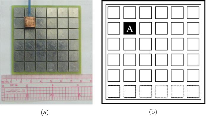
The 10 mm copper target (shaded rectangle) is placed 0, 5 and 10 mm distant from the electrode array in position A. (a) Electrode array and target. (b) Target position

Since we only seek to reconstruct the admittivity distribution accurately in the region directly below the electrode array, only those voxels are included in the image. In the reconstructions shown, we make use of a reconstruction mesh with 20 × 20 × 10 voxels in the x, y and z planes, respectively, with fewer voxels used in the z direction because of the poor depth resolution in the mammography geometry. In our experiments, we place the target at depths of 0, 5 and 10 mm directly facing the electrode in position A in figure 4(b), where by a depth of 0 mm we mean that we place the inclusion as close to the electrode as possible, without touching the electrode directly. As in the forward model comparison above, we made use of 2048 basis functions in the solution of the forward problem for each current pattern, for both the ave-gap and complete models.

In solving the inverse problem we set r₁ and r₂ in (33) to 0.5, where we have made this choice as a trade-off between image smoothness and resolution. In our experimentation with these parameters, we have noted that NOSER-type regularization (specified by r₁) is superior to Tikhonov regularization (specified by r₂) alone in reconstructing images deep within the medium, but that a non-zero Tikhonov regularization parameter is necessary in order to avoid excessive surface artifacts in the reconstruction.

The results for the reconstruction of the target at depth 0 are shown in figure 5. At such a depth our sensitivity is so overwhelmingly high that the signal generated by the target is much greater than the error caused by the incorrect modeling assumptions in the ave-gap model, and thus the reconstructions made assuming an ave-gap model or a complete electrode model are excellent and very similar to one another.

Figure 5.

Reconstructed static images. The 10 mm copper target was placed 0 mm distant from the electrode array in position A. The range of conductivity values is given in mS m⁻¹. (a) Reconstructed images by an ave-gap model. (b) Reconstructed images by a complete model.

In figure 6, the target is placed at a distance of 5 mm from the top electrode array. The ave-gap reconstruction, displayed in figure 6(a) shows a characteristic low spatial-frequency checkerboard pattern near the top and bottom electrode arrays, while this artifact is less evident in the reconstruction where the complete electrode model has been used, figure 6(b). We note in passing that the differences between the two models affect both the reconstruction data and the Jacobian matrix, D and J, in (33). In figure 7 the reconstructions are shown where the target has been placed at a distance of 10 mm from the top electrode array. We again see a characteristic pattern of artifacts, strongest in the slice immediately nearest the electrodes, but highly visible in other slices as well, in the ave-gap reconstruction, figure 7(a), which are again less visible in the complete electrode model reconstruction, figure 7(b). However, the reconstructed contrast of the inclusion is higher for the ave-gap reconstruction.

Figure 6.

Reconstructed static images. The 10 mm copper target was placed 5 mm distant from the electrode array in position A. The range of conductivity values is given in mS m⁻¹. (a) Reconstructed images by an ave-gap model. (b) Reconstructed images by a complete model.

Figure 7.

Reconstructed static images. The 10 mm copper target was placed 10 mm distant from the electrode array in position A. The range of conductivity values is given in mS m⁻¹. (a) Reconstructed images by an ave-gap model. (b) Reconstructed images by a complete model.

4. Conclusions

In this study, we have experimentally investigated the importance of accurately modeling the electrode–medium interface for EIT in a parallel-plane mammography geometry. Where the exact same basis functions are used for both models, the complete model gives a considerable improvement in modeling accuracy. In addition, when the same reconstruction algorithm and regularization parameters are used for both models, the complete electrode model gives a qualitatively more appealing result, with fewer artifacts in the slices nearest to the electrodes. We have also shown the analytical solution for the ave-gap method in the mammography geometry and demonstrated a practical semi-analytic method for computing the solution of the complete electrode model in this geometry as well.

References

- Barber DC, Brown BH. Applied potential tomography. J. Phys. E.: Sci. Instrum. 1984;17:723–33. [Google Scholar]
- Blue RS, Isaacson D, Newell JC. Real-time three-dimensional electrical impedance imaging. Physiol. Meas. 2000;21:15–26. doi: 10.1088/0967-3334/21/1/303. [DOI] [PubMed] [Google Scholar]
- Cheney M, Isaacson D, Newell JC, Simske S, Goble J. NOSER: an algorithm for solving the inverse conductivity problem. Int. J. Imaging Syst. Technol. 1990;2:65–75. doi: 10.1002/ima.1850020203. [DOI] [PMC free article] [PubMed] [Google Scholar]
- Cheng KS, Isaacson D, Newell JC, Gisser DG. Electrode models for electric current computed tomography. IEEE Trans. Biomed. Eng. 1989;36:918–24. doi: 10.1109/10.35300. [DOI] [PMC free article] [PubMed] [Google Scholar]
- Cherepenin V, Karpov A, Korjenevsky A, Kornienko V, Mazaletskaya A, Mazourov D, Meister D. A 3D electrical impedance tomography (EIT) system for breast cancer detection. Physiol. Meas. 2001;22:9–18. doi: 10.1088/0967-3334/22/1/302. [DOI] [PubMed] [Google Scholar]
- Choi MH, Kao T-J, Isaacson D, Saulnier GJ, Newell JC. A reconstruction algorithm for breast cancer imaging with electrical impedance tomography in mammography geometry. IEEE Trans. Biomed. Eng. 2007;54:700–10. doi: 10.1109/TBME.2006.890139. [DOI] [PMC free article] [PubMed] [Google Scholar]
- Elmore JG, Barton MB, Moceri VM, Polk S, Arena PJ, Fletcher SW. Ten-year risk of false positive screening mammograms and clinical breast examinations. N. Engl. J. Med. 1998;338:1089–96. doi: 10.1056/NEJM199804163381601. [DOI] [PubMed] [Google Scholar]
- Feuer EJ, Wun LM, Boring CC, Flanders WD, Timmel MJ, Tong T. The lifetime risk of developing breast cancer. J. Natl. Cancer Inst. 1993;85:892–7. doi: 10.1093/jnci/85.11.892. [DOI] [PubMed] [Google Scholar]
- Heikkinen LM, Vilhunen T, West RM, Vauhkonen M. Simultaneous reconstruction of electrode contact impedances and internal electrical properties: II. Laboratory experiments. Meas. Sci. Technol. 2002;13:1855–61. [Google Scholar]
- Isaacson D. Distinguishability of conductivities by electric current computed tomography. IEEE Trans. Med. Imaging. 1986;MI-5:92–5. doi: 10.1109/TMI.1986.4307752. [DOI] [PubMed] [Google Scholar]
- Jossinet J. The impedivity of freshly excised human breast tissue. Physiol. Meas. 1998;19:61–75. doi: 10.1088/0967-3334/19/1/006. [DOI] [PubMed] [Google Scholar]
- Kao T-J, Newell JC, Saulnier GJ, Isaacson D. Distinguishability of inhomogeneities using planar electrode arrays and different patterns of applied excitation. Physiol. Meas. 2003;24:403–11. doi: 10.1088/0967-3334/24/2/352. [DOI] [PubMed] [Google Scholar]
- Kerlikowske K, Grady D, Barclay J, Sickles EA, Ernster V. Effect of age, breast density, and family history on the sensitivity of first screening mammography. JAMA. 1996;276:33–8. [PubMed] [Google Scholar]
- Kerner TE, Paulsen KD, Hartov A, Soho SK, Poplack SP. Electrical impedance spectroscopy of the breast: clinical imaging results in 26 subjects. IEEE Trans. Med. Imaging. 2002;21:638–45. doi: 10.1109/tmi.2002.800606. [DOI] [PubMed] [Google Scholar]
- Kim BS, Kim KY, Kao T-J, Newell JC, Isaacson D, Saulnier GJ. Dynamic electrical impedance imaging of a chest phantom using the Kalman filter. Physiol. Meas. 2006;27:81–91. doi: 10.1088/0967-3334/27/5/S07. [DOI] [PMC free article] [PubMed] [Google Scholar]
- Kunst PWA, Noordegraaf AV, Hoekstra OS, Postmus PE, de Vries PMJM. Ventilation and perfusion imaging by electrical impedance tomography: a comparison with radionuclide scanning. Physiol. Meas. 1998;19:481–90. doi: 10.1088/0967-3334/19/4/003. [DOI] [PubMed] [Google Scholar]
- Liu N, Saulnier GJ, Newell JC, Isaacson D, Kao T-J. ACT4: a high-precision, multi-frequency electrical impedance tomograph. Proc. 6th Conf. on Biomedical Applications of Electrical Impedance Tomography; University College London, UK. 22–24 June.2005. [Google Scholar]
- Mueller JL, Isaacson D, Newell JC. A reconstruction algorithm for electrical impedance tomography data collected on rectangular electrode arrays. IEEE Trans. Biomed. Eng. 1999;46:1379–86. doi: 10.1109/10.797998. [DOI] [PubMed] [Google Scholar]
- Nystrom L, Rutqvist LE, Wall S, Lindgren A, Lindqvist M, Ryden S, Andersson I, Bjurstam N, Fagerberg G, Frisell J. Breast cancer screening with mammography: overview of Swedish randomised trials. Lancet. 1993;341:973–8. doi: 10.1016/0140-6736(93)91067-v. [DOI] [PubMed] [Google Scholar]
- Ross AS. PhD Thesis. Rensselaer Polytechnic Institute, Troy; New York, USA: 2003. An adaptive current tomograph for breast cancer detection. [Google Scholar]
- Somersalo E, Cheney M, Isaacson D. Existence and uniqueness for electrode models for electric current computed tomography. SIAM J. Appl. Math. 1992;52:1023–40. [Google Scholar]
- Tidswell T, Gibson A, Bayford RH, Holder DS. Three-dimensional electrical impedance tomography of human brain activity. Neuroimage. 2001;13:283–94. doi: 10.1006/nimg.2000.0698. [DOI] [PubMed] [Google Scholar]
- Vauhkonen M, Vadász D, Karjalainen PA, Somersalo E, Kaipio JP. Tikhonov regularization and prior information in electrical impedance tomography. IEEE Trans. Med. Imaging. 1998;17:285–93. doi: 10.1109/42.700740. [DOI] [PubMed] [Google Scholar]
- Vauhkonen PJ, Vauhkonen M, Savolainen T, Kaipio JP. Three-dimensional electrical impedance tomography based on the complete electrode model. IEEE Trans. Biomed. Eng. 1999;46:1150–60. doi: 10.1109/10.784147. [DOI] [PubMed] [Google Scholar]
- Vilhunen T, Kaipio JP, Vauhkonen PJ, Savolainen T, Vauhkonen M. Simultaneous reconstruction of electrode contact impedances and internal electrical properties: I. Theory. Meas. Sci. Technol. 2002;13:1848–54. [Google Scholar]