Measuring Tortuosity of the Intracerebral Vasculature from MRA Images

Abstract

The clinical recognition of abnormal vascular tortuosity, or excessive bending, twisting, and winding, is important to the diagnosis of many diseases. Automated detection and quantitation of abnormal vascular tortuosity from three-dimensional (3D) medical image data would therefore be of value. However, previous research has centered primarily upon 2D analysis of the special subset of vessels whose paths are normally close to straight.

This report provides the first 3D tortuosity analysis of clusters of vessels within the normally tortuous intracerebral circulation. We define three different clinical patterns of abnormal tortuosity. We extend into 3D two tortuosity metrics previously reported as useful in analyzing 2D images and describe a new metric that incorporates counts of minima of total curvature. We extract vessels from MRA data, map corresponding anatomical regions between sets of normal patients and patients with known pathology, and evaluate the three tortuosity metrics for ability to detect each type of abnormality within the region of interest.

We conclude that the new tortuosity metric appears to be the most effective in detecting several types of abnormalities. However, one of the other metrics, based on a sum of curvature magnitudes, may be more effective in recognizing tightly coiled, “corkscrew” vessels associated with malignant tumors.

I. Introduction

MANY diseases affect blood vessel morphology. To the clinician, one of the most important measures of vessel shape is “tortuosity”. Estimating the tortuosity of individual large vessels is important when evaluating atherosclerosis, for example, since abnormal tortuosity is associated both with an increased risk of stroke and with failure of endovascular therapy [1], [2]. Disease processes such as diabetes, hypertension and the vasculopathies affect the circulation globally and produce small, abnormally tortuous vessels that may be the primary cause of intracerebral hemorrhage [3], [4], [5]. Of particular interest, malignant tumors and vascular malformations each produce localized clusters of abnormally tortuous vessels, and successful treatment with anti-angiogenic agents reduces the tortuosity of the abnormal vessels [6]. An objective method of quantifying the tortuosity both of individual vessels and of groups of vessels would thus be of value in the diagnosis, staging, and therapeutic monitoring of a variety of diseases.

Webster’s dictionary defines “tortuosity” as “full of twists, turns; crooked” [7]. How best to transform the clinician’s intuitive perception of abnormal twisting, turning, and crookedness into a specific metric is not clear, however. An ideal method of detecting abnormal tortuosity of the three-dimensional (3D) intracerebral vasculature would be applicable to 3D image data and capable of defining vessels of abnormal tortuosity against a backdrop of normally tortuous vessels. However, previous research has been largely limited to the small subset of vessels whose normal configurations are close to straight. Moreover, most previous work has focused upon 2D images of retinal vessels, and thus has analyzed tortuosity only in 2D.

This paper describes early work toward analysis of the 3D tortuosity of the intracerebral vasculature. Such analysis is difficult not only because the intracerebral vasculature is inherently tortuous, but also because normal vessels do not conform to a single pattern. Indeed, some normal intracerebral vessels are straight, some meander in broad curves, some form coils, and some oscillate. Moreover, a normal intracerebral vessel may possess one type of configuration in one location and another configuration elsewhere. It is therefore impossible to provide a single, global shape description that defines all normal intracerebral vessels. To further complicate the problem, the variability of the intracerebral circulation precludes a one-to-one mapping of individual vessels between patients for more than a few, large, named vessels.

The focus of this paper is upon evaluation of the relative efficacy of three tortuosity metrics in discriminating normal from abnormal intracerebral vessels. Two of these metrics have previously been described as useful in evaluating 2D image data. We extend each of these methods to 3D. The third metric is new and incorporates a count of loci exhibiting minima of local curvature. This report also defines three different clinical patterns of abnormal tortuosity. We then test each metric for its ability to detect each type of abnormality, using comparison of diseased vessels to vessels located in the same anatomical region of normal patients. We conclude that the new metric appears to be the most sensitive in detecting two types of abnormal tortuosity. The third type of tortuosity, characterized by tight coils, may be best detected by a method that sums curvature magnitudes.

II. Background

A. Tortuosity metrics

Little information is available on the evaluation of vascular tortuosity in 3D. Nevertheless, many investigators have investigated vascular tortuosity in 2D and under the specific condition in which the definition of normal is known to be close to a straight line. The majority of publications have centered upon retinopathy of prematurity. The most common measure of vascular tortuosity in 2D images has been the “distance metric”, which provides a ratio of the actual path length to the linear distance between curve endpoints [8], [9], [10], [11], [12]. As noted by Capowski [13], however, the disadvantage of this approach is that it is insensitive to the frequency with which a vessel “wiggles”. Worse, when analyzing the intracerebral vasculature, a problem with the distance metric is that it often assigns a higher tortuosity value to a normal, long, “S” or “U” shaped vessel than to a shorter, abnormal vessel possessing tight coils or high frequency oscillations.

Capowski [13] describes a tortuosity measure based on estimating the likely spatial frequency of the pathology in question and then calculating the distance metric over vessel segments of appropriate length. We agree with Capowski that frequency measures could be useful in distinguishing normal from some types of abnormal vessels. However, his specific approach is difficult to implement when both normal and abnormal vessels exhibit varying spatial configurations.

Smedby [9] postulates 4 tortuosity measures, one of which counts inflection points. This idea is appealing because it incorporates frequency information into the definition of tortuosity. However, Smedby does not describe how to normalize frequency count for vessel length or how to generalize the approach to 3D. The current article builds upon this idea, however, and describes a new method of tortuosity calculation that combines a count of 3D “inflection points” with the distance metric.

Hart [12] describes 9 different tortuosity metrics and compares them to opthalmologists’ qualitative assessments of the tortuosity of retinal vessels as seen in 2D images. Of note, Hart’s opthalmologists preferred a metric that integrates the total curvature magnitude along a curve and then normalizes by path length. We have used a geometrical approach to extend this sum of curvature magnitudes approach to 3D, and we include it as one of the metrics to be evaluated.

One problem when discussing abnormal tortuosity is that some disease states, such as retinopathy of prematurity, produce sinusoidal curves [13]. In such cases, the terms “amplitude” and “frequency” have obvious meaning. However, other diseases may induce corkscrew vessels or a conglomeration of erratically twisted vessels. In such cases, the terms “amplitude” and “frequency” become unclear.

In this paper, we use the term “coil” to describe a corkscrew curve (helix). We employ the word “frequency” to indicate both the frequency of sinusoidal curves and the frequency with which a coil completes a full turn around a cylinder whose axis is of unit length. We employ the word “amplitude” to indicate both the amplitude of sinusoidal curves and the radius of a coil.

B. Vessel segmentation

Calculation of tortuosity for an individual vessel or across a population of vessels requires definition of each vessel’s medial axis. Many groups have described methods of segmenting vessels from MRA [14], [15], [16], [17], [18], [19], [20], [21], [22], [23], [24], [25], [26]. Aylward [27] reviews various vessel segmentation methods. However, the approaches outlined in the current report are applicable to any method of vessel extraction from 3D image data as long as the technique provides an ordered, regularly spaced set of 3D points describing each vessel’s skeleton curve.

C. Clinical patterns of abnormality

In order to evaluate any tortuosity metric for clinical use, it is necessary to test it against curves that are known to be abnormal. This paper defines three patterns of abnormal 3D vascular tortuosity, each associated with a different disease process. For lack of better terminology, these abnormal patterns are called Types I, II, and III. Table 1 provides a brief summary of these three types of abnormality, each of which is discussed in more detail below.

Table 1.

Summary of abnormal tortuosity types.

Abnormal Tortuosity Types
Type	Length	Amp	Freq	Comment
I	Long	High	Low	Sinuous curves in long, normally straight vessels
II	Variable	Med	Med	Tightly packed cluster; erratic directional changes
III	Variable	Low	High	Tight coils or sine waves

Length= length of affected vessels. Amp = amplitude. Freq = frequency. Med = medium. Definitions of frequency and amplitude are given in section IIA.

Type I is the simplest type of abnormality, and has been analyzed by many investigators investigating vascular tortuosity in 2D image data. Type I tortuosity abnormalities occur when a vessel elongates so that a normally straight or gently curved vessel begins to exhibit a “C” or “S” or “repeated S” configuration. The disease occurs with aging, hypertension, atherosclerosis, retinal disease of prematurity, and with a variety of hereditary diseases that affect the vessel wall. This type of abnormal tortuosity is also associated with risk of vessel thrombosis and stroke, making quantitative evaluation of type I tortuosity of particular clinical interest.

Figure 1 illustrates the paired vertebral arteries and the basilar artery of a patient with a severely tortuous basilar artery. The abnormal case is shown at far left, and the vessels of three normal subjects at right. Arrows point to the basilar artery, which, in the abnormal subject, was so severely tortuous that it produced cranial nerve deficits.

Fig 1.

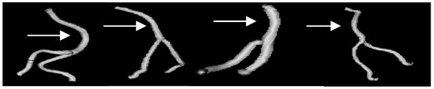
Type I tortuosity abnormality. An abnormal basilar artery is shown at far left. The three images to right provide examples of three normal vertebro-basilar systems. An arrow points to the basilar artery.

Type II abnormalities occur in the presence of highly vascular tumors and within the nidi of arteriovenous malformations (AVMs). Abnormal vessels are packed within a small volume of space and exhibit frequent and unpredictable changes of direction. Successful treatment with anti-angiogenic factors reduces the tortuosity of the vessels within the affected region [6], suggesting that quantitative measurements of tortuosity could be helpful in monitoring treatment. Figure 2 provides an example of an AVM nidus.

Fig. 2.

Type II tortuosity abnormality. Curved vessels of variable length are packed together. Vessels within the tumor nidus are red; vessels supplying or passing through the nidus are gold, and normal vessels outside the nidus are blue. The nidus, containing type II tortuosity vessels, is volume rendered at full opacity at left, at partial opacity at center, and the vessels are shown alone at right.

Type III abnormalities are apparent in malignant brain tumors when imaged by high resolution MR. These abnormal vessels are of variable length, may be straight or curved, but exhibit high frequency coils. The ability to quantitate such abnormalities has the interesting potential of identifying foci of active tumor growth as well as providing a means of monitoring anti-tumor therapy. Figure 3 provides an example of a patient with a malignant glioma. Vessels entirely within the tumor are red, vessels partially within the tumor are gold, and normal vessels outside the tumor are blue. The vessels located entirely or partially within the tumor exhibit high frequency, low amplitude coils or sinusoidal patterns.

Fig. 3.

Type III tortuosity abnormality. High frequency coils or sinusoidal curves are present in vessels that traverse or lie within a malignant glioma. Red vessels are located entirely within the tumor, gold vessels traverse the tumor, and blue vessels are presumably normal vessels entirely outside the tumor. The tumor, containing type III tortuosity vessels, is volume rendered at full opacity (left), at partial opacity (center) and the vessels are shown alone at right.

III. Methods

A. Image acquisition and patient selection

All patients were imaged by 3D, time-of-flight MRA using a quadrature head coil. Off resonance (1500 Hz) magnetization transfer suppression (75 Hz) was used to further suppress background stationary tissue. Tumor and AVM patients additionally underwent T1, gadolinium enhanced MR scans.

Type I tortuosity abnormalities are exemplified by a patient in whom radiologists identified the basilar artery as abnormal (Figure 1). Type II tortuosity abnormalities (Figure 2) are exemplified by three AVM patients. Type III tortuosity errors (Figure 3) are exemplified by three patients with malignant gliomas. Eleven normal subjects served as controls.

Our institution is currently in transition between an older imaging protocol that acquired MRA data on a Siemens 1.5 T Vision unit at 256 × 256 × 90+ voxel resolution (0.9 × 0.9 × 1 mm³) and a higher resolution protocol of 512 × 512 × 90+ voxels (0.4 × 0.4 × 1mm³) available both on the 1.5 T unit and on a newer Siemens 3T Allegra unit.

We first noted the presence of tortuosity Type III within malignant gliomas only after the adoption of the higher resolution protocol, and, to date, all malignant glioma patients imaged at high resolution on either of our MR scanners have shown the same abnormalities. It therefore seems possible that image resolution can affect the assessment of some kinds of tortuosity. This study therefore only compares normal and abnormal images obtained at the same spatial resolution.

In this article, all tumor and AVM images were acquired at high resolution, with two of the three tumor cases and one of the three AVM patients scanned on the 3T unit. Each abnormal case is compared to those of eleven normal volunteers, each imaged at high resolution on the 3T unit.

The patient with an abnormally tortuous basilar artery was imaged at low resolution. We do not have a database of normal volunteers imaged at low resolution, so this study compares the abnormal basilar artery to the basilar arteries of eleven subjects also imaged at low resolution on the same 1.5 T unit. These “normal” patients actually suffered from a variety of diseases but had no disease of the basilar artery.

B. Vessel and tumor segmentation

We employ the vessel segmentation method of Aylward [27]. Vessel extraction involves 3 steps: definition of a seed point, automatic extraction of an image intensity ridge representing the vessel’s central skeleton, and automatic determination of vessel width at each skeleton point. The output of the program is a set of directed, 4-dimensional points indicating the (x,y,z) spatial position of each sequential vessel skeleton point and an associated radius at each point. The vessel skeleton is defined as a spline, which we subsequently sample at regularly spaced intervals. We have experimented with different sampling rates using synthetic data, and find that for purposes of tortuosity evaluation a sampling distance of one voxel allows adequate estimation of arc length while avoiding noise that can appear with sub-voxel sampling.

The output of the vessel segmentation program is postprocessed to provide a set of vessel “trees”, using an automated method that links vessels on the basis of distance and the existence of supporting image intensity information [28]. The same program possesses editing tools that can turn off subtrees and clip individual vessels proximally or distally.

The surface of each tumor or AVM nidus was defined from gadolinium-enhanced MR images using Dr. Gerig’s IRIS, a suite of tools that permits partially manual segmentation of tumors via polygon drawing and filling on orthogonal cuts through an image volume [29]. IRIS outputs a mask file of the same size as the input file. In this mask file, each voxel has a numeric label indicating the number of the segmented object associated with that voxel. If the voxel does not lie within a segmented object the voxel is assigned a value of 0.

C. Image registration

To compare focally abnormal vascular images with a set of normal images it is desirable either to identify corresponding vessels or to define corresponding anatomical regions across patients. The basilar artery is a large vessel easily identifiable from patient to patient. For analysis of basilar artery tortuosity, the basilar artery was therefore identified in each subject and was clipped proximally at the junction of the vertebrals and distally at the takeoff of the posterior cerebrals. Equivalent vascular segments could thus be compared across patients without need for explicit registration of the images as a whole.

The abnormal vasculature of tumors and AVMs involves multiple unnamed vessels that cannot be mapped on a one-to-one basis from patient to patient, however. For patients with AVMs or tumors, we therefore defined the lesion boundaries and analyzed the tortuosity of all vessels and vessel segments lying within these boundaries. This same anatomical region was then defined in each of the eleven normal patients, and the tortuosity of all vessels and vessel segments contained within the region of interest was calculated from the unaltered image data of each normal subject.

All image registrations were performed using Drs. Rueckert and Schnabel’s mutual information-based registration program rview2 [30], [31], [32]. This program permits rigid, affine, and fully deformable registration, and, for rigid and affine registrations, the output can be saved as a file readily converted to a registration matrix. For the purposes of this project, we employed only rigid and full affine registrations and saved the output matrices. Settings for rigid and affine registrations included bins = 64, iterations = 100, steps = 4, step length = 2.0, levels = 3, and similarity measure = normalized mutual information.

For each patient with a lesion, the gadolinium-enhanced MR was registered rigidly with the same patient’s MRA. Since the mask file and gadolinium-enhanced MR share the same coordinate system and since segmented vessels share the MRA’s coordinate system, the same matrix relates the patient’s segmented tumor and segmented vessels.

All MRAs were then registered, using a full affine transformation, with the MRA of the first patient in the normal patient database. Lesion coordinates from any abnormal patient could then be transformed into the coordinate system of any other patient’s MRA via a set of matrix multiplications. The mask file was then resliced into the coordinate system of each target MRA, vessels traversing the region of interest in the target MRA were clipped, and tortuosity analysis was applied only to those vessels and vessel segments lying within the region of interest. This approach therefore determines tortuosity values only within the undeformed space of each target MRA, with deformable mapping of the region of interest to each target MRA. Figures 2 and 3 illustrate definition of vessels relative to the surface of a registered lesion.

D. Tortuosity metrics

This report evaluates three different tortuosity metrics—the “distance metric” (DM), the “sum of angles metric” (SOAM), and the “inflection count metric” (ICM). As implemented here, all calculations take as input a set of ordered 3D points indicating the spatial position of each vessel skeleton, regularly sampled at intervals of the length of one voxel. We have employed a geometric approach when defining tortuosity measures. Vectors are indicated in bold font and points in italicized font. The difference between two points produces a vector. The notation uses “n” to indicate the number of points in a curve and P_k to indicate vessel skeleton point “k”. P₀ is the first point of any curve and P_{n −1} the last point.

1) Distance metric (DM)

As previously noted, the distance metric is the approach that has been used most frequently to evaluate vascular tortuosity in 2D. It provides a ratio between the actual path length of a meandering curve and the linear distance between endpoints (Figure 4). Extension of the approach to 3D is straightforward. The distance metric produces a dimensionless number.

Fig. 4.

Distance metric. The sum of distances between adjacent 3D points along the actual vessel path (short arrows) is divided by the length of the straight path between the first and last 3D points (long line).

2) Inflection count metric (ICM)

Although the DM calculates how far a path deviates from that of a straight line, its usefulness is limited as it may assign the same tortuosity value to a large, gentle “C” curve as to a much more tortuous vessel that makes abrupt changes in direction. We therefore propose a modification to the DM that multiplies the DM by the number of the curve’s “inflection points”. For a 3D space curve, we define an inflection point as a locus that exhibits a minimum of total curvature. In particular, the Normal and Binormal axes of the Frenet frame [33] change orientation by close to 180° as the frame passes through an inflection point. As a result, one can search for 3D inflection points by identifying large local maxima of the dot product ΔN • ΔN, where N is the unit vector representing the Frenet normal axis, and ΔN represents the difference of the normal axes associated with points P_k and P_k−1.

We use a geometric implementation of the Frenet frame. Bloomenthal [34] describes a similar geometric derivation. Figure 5 illustrates computation of the Frenet frame from a set of ordered, 3D points that define a vessel skeleton curve.

Fig. 5.

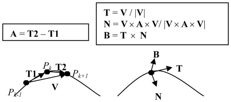
Frenet frame. Left: determination of velocity (V) and acceleration (A) vectors. Right: derivation of the Frenet frame given the V and A vectors.

The left side of Figure 5 illustrates a space curve. The velocity vector V at point P_k can be approximated by the vector between the points P_k−1 and P_k+1. The acceleration vector A at point P_k is approximated by subtracting the vector T1 from the vector T2. The right side of Figure 5 illustrates derivation of the Frenet frame coordinates from the velocity and acceleration vectors. The Frenet tangent axis, T, is the normalized velocity vector. The Frenet normal axis, N, is derived by crossing the velocity and acceleration vectors (producing an out of plane vector at right angles to both), and then crossing that vector with the velocity vector and normalizing. The result is a unit vector in the same plane as both the velocity and acceleration vectors, and orthogonal to the tangent vector T. The third, binormal axis (B) can then be derived, if desired, by crossing T and N.

One problem with the Frenet frame is that it is undefined whenever the acceleration vector has no length, as occurs at inflection points or during passage over a straight line. We handle this problem by checking the length of the acceleration vector, and if this length is less than 10⁻⁶ cm we simply skip the point and redefine the frame at the next vessel point.

Figure 6 provides a synthetic, test example of a sine wave possessing 3 inflection points and 4 extrema. The data is processed in 3D. In the upper picture, the Frenet T and N axis vectors are drawn at various points along the space curve. The direction of the unit N vector (white arrow) rotates close to 180° after passing through each inflection point (oval), so that the length of ΔN at these locations is close to 2. In the lower picture, the squared length of each ΔN is graphed against time. As shown here, passage through an inflection point produces a large signal with ΔN • ΔN approximately equal to 4.0, whereas the values at other locations are in the range of 10⁻² to 10⁻⁸. The four barely discernible, tiny peaks occurring midway between the huge inflection point peaks have a value of 0.01, and correspond to the space curve’s four minima and maxima, where the N vector changes orientation rapidly without “flipping over”. Passage through an inflection point is recognized by searching for local maxima of ΔN•ΔN when ΔN•ΔN is greater than 1.0.

Fig. 6.

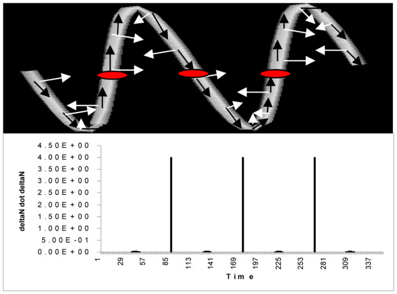
Recognition of inflection points in a 3D test object. Above: The Frenet T (black arrows) and Frenet N (white arrows) vectors are drawn at various points along the curve. Passage of the frame through an inflection point (red oval) produces close to a 180° rotation in the orientation of the N vectors. Right: Graph of ΔN•ΔN against time. The three huge peaks correspond to passage of the frame through an inflection point. The 4 tiny peaks correspond to the space curve’s extrema.

If the number of inflection points is 0, the ICM will report no tortuosity even if the curve makes a large arc. We therefore add 1 to the calculated inflection count. Both a straight line and a coil are thus reported as having inflection counts of 1.

The ICM multiplies the DM by the inflection count, using a minimum inflection count of 1. The ICM thus will never have a value less than the DM and will always be an integral multiple of the DM. As compared to the DM, however, the ICM is more sensitive to oscillating curves and will report an oscillating curve as more tortuous than a curve with the same total length and endpoints but that makes a single, large, “C”.

3) Sum of angles metric (SOAM)

A disadvantage of both the DM and the ICM is that neither method handles tight coils well. Since high frequency, low amplitude coils do not add greatly to total path length, the DM regards such highly tortuous curves as close to straight and assigns a low tortuosity value. As coils do not contain inflection points, the ICM does no better than the DM when analyzing coils and reports the same tortuosity values.

An alternative approach is to integrate total curvature along a curve and to normalize by path length. The approach described below provides a 3D, geometrically based variant of the curvature integration method described by Hart [12].

As implemented here (Figure 7), the in-plane curvature at point P_k is estimated by calculating the vector T1 between the points P_k−1 and P_k, and the vector T2 between points P_k and P_k+1. The vectors are normalized, the dot product obtained, and the arccosine calculated so as to provide an angle between the two vectors. If the three points are collinear, the in-plane angle will thus be reported as 0. If the three points are close to collinear, the in-plane angle is small. If the three points define a sharp peak, the in-plane angle is large.

Fig. 7.

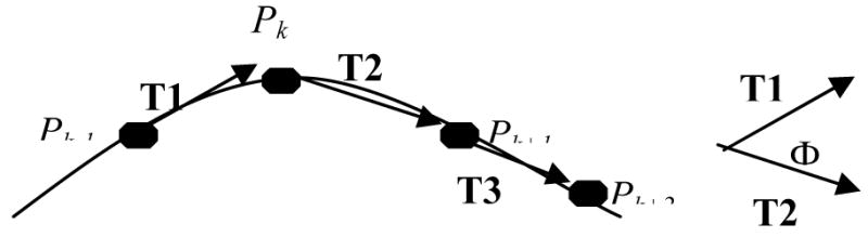
Calculation of the in-plane angle Φ at point P_k.

The torsion at point P_k is represented by the angle between the plane of the current osculating circle, whose surface normal is the normalized cross product of the vectors T1 and T2, and the surface normal of the subsequent osculating plane defined by points P_k, P_k+1, and P_k+2. Just as the Frenet Normal and Binormal axes reverse direction as the Frenet frame crosses an inflection point, the normals of two successive osculating planes will point in opposite directions when P_k and P_k+1 lie on opposite sides of an inflection point. Although it may ultimately be desirable to retain this feature as an additional measure of tortuosity, it is confusing to include points with torsional angles of 180° when analyzing a planar curve. For all analyses in this paper, we therefore assign a torsional angle of 0 (rather than 180°) whenever the frame crosses an inflection point.

As outlined above, both the in-plane and the torsional angles are positive angles lying between 0 and 180°. A positive total angle of “curvature” at point P_k is calculated by taking the square root of the sum of the squares of the inplane angle and of the torsional angle. The total angles are summed for each valid point in the curve, and the result is normalized by dividing by the total curve length. Results are given in radians/cm.

For any point P_k the vectors T1, T2 and T3 are defined by:

$$\begin{array}{l}\mathbf{T}\mathbf{1}=P_k-P_{k-1}\\ \mathbf{T}\mathbf{2}=P_{k+1}-P_k\\ \mathbf{T}\mathbf{3}=P_{k+2}-P_{k+1}\end{array}$$

The in-plane angle at point P_k (IP_k) and the torsional angle TP_k are given by:the following equations, where TP_k, IP_k € [0, Π].

$$\begin{array}{l}{\text{IP}}_{\text{k}}={cos}^{-1}((\mathbf{T}\mathbf{1}/\mid \mathbf{T}\mathbf{1}\mid )•(\mathbf{T}\mathbf{2}/\mid \mathbf{T}\mathbf{2}\mid ))\\ {\text{TP}}_{\text{k}}={cos}^{-1}((\mathbf{T}\mathbf{1}\times \mathbf{T}\mathbf{2}/\mid \mathbf{T}\mathbf{1}\times \mathbf{T}\mathbf{2}\mid )•(\mathbf{T}\mathbf{2}\times \mathbf{T}\mathbf{3}/\mid \mathbf{T}\mathbf{2}\times \mathbf{T}\mathbf{3}\mid ).\end{array}$$

The total angle CP_k at point P_k is then

$${\text{CP}}_{\text{k}}=\sqrt{(\text{IPk}\times \text{IPk})+(\text{TPk}\times \text{TPk})}$$

The sum of angles metric calculates the total tortousity of the curve as

$$\text{SOAM}=(\sum _{\text{k}=1}^{\text{n}-3}{\text{CP}}_{\text{k}})/(\sum _{\text{k}=1}^{\text{n}-1}\mid P_k-P_{k-1}\mid )$$

E. Tortuosity calculations in phantom data

The differences between the three tortuosity metrics are most clearly explained using synthetic data. Table 2 provides the results of analysis of simple curves in which one variable is manipulated at a time. Each trio of rows manipulates one variable and orders the curves from least to most tortuous. Definitions of “frequency” and “amplitude” are given in section IIA. We assume that, for a given total path length, a higher frequency curve (more inflection points or a more tightly wound coil) should be assigned a higher tortuosity value. We also assume that, for a given frequency, a curve of greater amplitude should be assigned a higher tortuosity value.

Table 2.

Tortuosity measurements using synthetic data

Tortuosity Measurements Using Synthetic Data
	Freq	Amp	Len	DM	ICM	SOAM
Sine	3	10.0	13.9	1.6	9.7	0.9
Sine	10	3.0	13.9	1.6	32.3	3.1
Sine	20	1.5	13.9	1.6	64.7	6.2
Coil	3	6.3	13.9	1.5	1.5	1.3
Coil	10	1.9	13.9	1.5	1.5	4.5
Coil	20	0.94	13.9	1.5	1.5	9.2
Sine	3	10.0	13.9	1.6	9.7	0.9
Sine	3	20.0	22.9	2.7	16.0	0.7
Sine	3	40.0	42.6	5.0	29.7	0.4
Coil	3	6.3	13.9	1.5	1.5	1.3
Coil	3	20.0	33.7	3.6	3.6	0.6
Coil	3	40.0	65.3	6.9	6.9	0.3

Amp = amplitude. Len = total curve length (cm). Each trio of curves manipulates one variable and presents curves in the order of least to most tortuous. Each curve is analyzed by all three tortuosity metrics. Bold results indicate the metrics that appear to handle the manipulated variable correctly.

The first three rows of Table 2 provide results for low, medium, and high frequency sine waves, each of which begins in the same start voxel and ends in the same end voxel. Via adjustment of amplitude, each sine wave also has the same total path length. The sine wave of highest frequency is therefore the most “wiggly”, although it also has the lowest amplitude. The DM is incapable of distinguishing between such curves, and reports an identical tortuosity value for each. Both the ICM and the SOAM metric, however, correctly assign a higher tortuosity to curves of higher frequency.

The second three rows of Table 2 provide results for low, medium, and high frequency coils, each of which begins in the same start voxel and ends in the same end voxel. Via adjustment of amplitude, each coil has the same total path length. The coil of highest frequency therefore is the most “wiggly”, although it also has the lowest amplitude. Similar to the sine wave example above, the DM is incapable of distinguishing between the three curves and assigns the same tortuosity value to each. As coils do not have inflection points, the ICM is also not capable of distinguishing between curves and reports results identical to that of the DM. Only the SOAM is capable of correctly distinguishing between the three curves, correctly assigning the highest tortuosity to the tightest coil of a given total path length.

The next three rows of Table 2 provide results for three sine waves, each of frequency 3, each of which begins and ends in the same begin/end voxels, but each of which is of different amplitude. The total path length thus increases from the first example to the last. Given a sine wave of given frequency, we view the curve of highest amplitude as the most tortuous. The SOAM performs poorly in this case, since higher amplitude curves have lower average curvature. However, both the DM and the ICM order the curve tortuosities correctly.

The final three rows in Table 2 analyze coils of a given frequency but of variable amplitude. Similar to the results for sine waves, both the DM and the ICM perform well, but the SOAM is ineffective because broad curves exhibit low average curvature.

In summary, results in these test data suggest that no single one of the tortuosity metrics under evaluation is capable of handling all situations correctly. The ICM provides, at minimum, equal information to the DM and moreover correctly ranks curves of equal lengths but of increasing frequency. The ICM therefore appears to be more powerful than the widely used DM. However, neither of these methods deals well with tight coils, and only the SOAM. appears capable of doing so effectively.

F. Analysis of multiple vessels

Any individual vessel can be assigned a tortuosity value by the methods described above. Our analyses must often deal with clusters of vessels, however. For the SOAM metric, it is straightforward to combine results for a cluster of vessels by summing the sum of angles calculated for each vessel and then dividing this composite sum by the total path length of all vessels. This provides an average angle per unit distance for that vessel cluster.

It is less obvious how to combine the results of the ICM and DM, however, as these two metrics involve a ratio of path lengths. Averaging the values given by a vessel cluster has the undesirable effect of weighting a very short vessel equally with a long one. For this paper, we therefore combine values for the DM by summing the numerators reported by the DM for each vessel and then dividing by the sum of the denominators. We take the same approach with the ICM. This approach provides a weighted average, with longer and more tortuous curves assigned a higher weight. Each metric thus reports a single value for each vessel cluster in each patient.

IV. Results

Results of analysis of medical images are presented by tortuosity type. Each section contains a table and a brief commentary. Each abnormal case is compared to a group of eleven normal subjects. Within each table, one, two, or three stars mark an abnormal value that is more than one, two, or three normal standard deviations from the normal mean. Results are presented for individual vessels in Table 3 and for groups of vessels in Tables 4 and 5.

Table 3.

Type 1 tortuosity of the basilar artery.

Type I Tortuosity Detection
	DM	ICM	SOAM
Abnormal Basilar	1.5***	2.9***	4.0
Normal Basilars	1.1 ± 0.1	1.3 ± 0.5	4.7 ± 1.9

Table 4.

Type II tortuosity abnormalities

Type II Tortuosity Detection
	DM	ICM	SOAM
Large AVM	1.6	325.1***	19.7
Normal	1.7 ± 0.6	39.2 ± 22.2	17.4 ± 1.9
Medium AVM	1.6***	75.8***	19.4
Normal	1.2 ± 0.1	12.8 ± 4.9	16.7 ± 3.4
Small AVM	1.5	50.1***	17.9
Normal	1.4 ± 0.2	24.0 ± 6.7	17.3 ± 2.3

AVM = arteriovenous malformation

Table 5.

Type III tortuosity abnormalities.

Type III Tortuosity Detection
	DM	ICM	SOAM
Tumor 1	1.2	20.3**	21.5*
Normal	1.2 ± 0.1	10.9 ± 4.0	16.3 ± 3.1
Tumor 2	1.3	22.7***	21.6**
Normal	1.2 ± 0.2	2.1 ± 1.1	12.5 ± 4.5
Tumor 3	1.4	64.9*	21.9*
Normal	1.5 ± 0.2	45.6 ± 13.6	16.8 ± 3.0

Table 3 provides results for a basilar artery exhibiting severe type I tortuosity. The abnormal artery and several normal examples are shown in Figure 1. Type I tortuosity abnormalities are characterized by meandering, broad curves. The curvature at any particular point is likely to be low, but the total length of the path may be great as compared to a straight line. As expected, both the DM and the ICM do well in detecting this type of abnormality while the SOAM does poorly. We believe that both the ICM and the DM provide an effective means of detecting type I tortuosity abnormalities.

B. Type II tortuosity

An example of type II tortuosity abnormality is shown in Figure 2. A dense nest of curved and erratically twisting vessels of variable length characterizes this type of pathology. Table 4 provides results of the analyses of three AVM patients. Results are compared to the vessels lying in the same anatomical region of 11 normal subjects.

As shown by Table 3, the distance metric often performs poorly with this type of pathology since many vessels are short. Indeed, the DM was able to flag only one of the three cases. The SOAM also has difficulty detecting type II abnormalities because the mix of broad and tight curves leads to an average curvature that is not very different from that of normal patients. The ICM, however, takes advantage of inflection counting to recognize the frequent changes of direction made by the “can of worms” that characterizes type II pathology. All results in patients with pathology were many standard deviations away from normal. We conclude that the ICM appears to be the method of choice when evaluating this type of lesion.

C. Type III tortuosity

Figure 3 provides an example of type III tortuosity. The affected vessels form high frequency coils of low amplitude. These patients also possess abnormal, serpiginous vessels that wiggle their way within the enhancing tumor rim. Table 5 provides results for the three tumor patients we have imaged at high resolution. Results in each patient are compared to the vessels lying in the same anatomical region of 11 normal subjects.

As discussed in section III E, the detection of tighly wound coils is very difficult for both the DM and the ICM, although the SOAM does better. Indeed, the SOAM was capable of differentiating abnormal from normal vessels in all three cases.

Malignant tumors also possess small nests of vessels somewhat similar to that of AVMs, and larger, serpiginous vessels may course within the tumor boundary (Fig. 3). Not surprisingly, the ICM is effective in flagging these types of abnormalities.

We are particularly interested in defining the characteristics of tumor vessels as seen by MR because of the potential of non-invasively quantitating vascular response to anti-angiogenesis treatment. We do not yet have enough subjects imaged at high resolution to draw definite conclusions about the best tortuosity metric for this group of patients, however. Nevertheless, the SOAM would seem to be the method of choice for characterizing the abnormal, tightly coiled vessels contained within all three of our patients with malignant tumors. The proportion of patients likely to possess additional longer, oscillating curves coursing around the surface of the tumor and best flagged by the ICM is unknown.

V. Discussion

Quantitating abnormal tortuosity of the intracerebral vasculature is difficult not only because intracerebral vessels are inherently tortuous but also because there is no single, geometrical description of a “normal” intracerebral vessel. The problem is compounded because the variability of the human intracerebral circulation precludes one-to-one mapping of individual vessels between different subjects for more than a few major named vessels.

This article is the first to attempt to quantitate the regional tortuosity of arbitrary portions of the 3D intracerebral vasculature. The results are encouraging. The distance metric (the tortuosity metric in most widespread use when analyzing 2D images) does not appear to be very useful for our purposes. However, the new inflection count method appears effective in recognizing two of the three types of abnormal tortuosity. A metric that sums angulations appears to be the most effective in recognizing the third type of abnormality, characterized by high frequency, low amplitude coils. Several points should be made about the methods, however.

First, our methods require defining similar anatomical regions across patients whose heads may be of different sizes and shapes. If one maps the MRA of a patient with a long, thin head to the MRA of a patient with a round head using only rigid registration, vessels in one image may lie outside of the second patient’s skull. This is obviously not an acceptable solution. If one uses either an affine or a fully deformable registration, however, one will deform the vessels of interest and thus alter tortuosity calculations. Although deformable mapping of all vasculature into a single patient’s coordinate system might reduce normal variability and thus be desirable, such mapping might also have undesirable effects. We do not yet know the optimal method of mapping vasculature between patients, and it is an active area of research of our group [35], [36].

For the current study we decided not to transform the vessels at all, but rather to deform the anatomical region of interest across patients. Vessels within this area of interest were then analyzed in their native states. Although this approach may ultimately be superseded by others, it seemed the safest approach under conditions in which registration of the vessels themselves would result in vessel deformation with a consequent unknown effect upon tortuosity calculations.

A second point is that the resolution at which the MRA data are obtained may affect tortuosity values. Type III tortuousity abnormalities, for example, may only be clearly evident on high-resolution images. We therefore have taken care to compare images of normal and abnormal subjects only when the images were obtained at the same resolution.

The particular vessel extraction protocol employed can also affect results. In particular, this paper describes a method that defines each vessel skeleton as a spline and then regularly samples that spline at a fixed distance of the size of one voxel. Use of a fixed sampling distance may underestimate total path length and thus affect the values reported by the DM and ICM. However, as noted by Koenderink [33], chords can be used to estimate arclength if they are short with respect to the radius of curvature. Indeed, if the chord is less than half the radius of curvature, deviation from the true arclength does not exceed one percent [33]. For a vessel to have a radius of curvature of two voxels, that vessel must make a sharp turn and possess a radius of less than half a voxel to be discriminated from the voxelized image data at all. Such vessels will be very faint because of volume averaging. It is doubtful that our vessel extraction method (or any other method) is capable of defining vessels of a much lower radius of curvature. A sampling distance of one point per voxel thus will not affect the calculation of arc length significantly. However, a long distance between sample points would obviously impede accurate length estimation as well as cause other problems such as inaccurate inflection counting.

All of the approaches analyzed in this article utilize the vessel central axis to compute tortuosity. We have not explicitly addressed the effect of vessel radius upon curvature, although a vessel’s radius clearly affects maximum allowable curvature. The mathematical relationship between curvature and radius is complex [37]. Nevertheless, it is an active area of research that could ultimately be of help to this project.

A final point is that vessel tortuosity is only one of several measures of vessel shape used by clinicians when recognizing and staging disease. Vessel diameter, branching patterns, and vascular density are also important. Determining such patterns in normal patients and in patients with disease could, in combination with tortuosity calculations, provide a new and very exciting means of quantitative image analysis helpful in diagnosing and evaluating a variety of diseases.

References

- 1.Kazanchyan PO, Popov VA, Gaponova Ye N, Rudakova TV. The diagnosis and treatment of pathological deformations of the carotid arteries. J Ang Vasc Surg. 2001;7:93–103. [Google Scholar]
- 2.Alazzaz A, Thornton J, Aletich VA, Debrun GM, Ausman JI, Charbel F. Intracranial percutaneous transluminal angioplasty for arteriosclerotic stenosis. Arch Neurol. 2000;57:1625–1630. doi: 10.1001/archneur.57.11.1625. [DOI] [PubMed] [Google Scholar]
- 3.Liem MD, Gzesh DJ, Flanders AE. MRI and angiographic diagnosis of lupus cerebral vasculitis. Diagnostic Neuroradiology. 1996;38:134–136. doi: 10.1007/BF00604798. [DOI] [PubMed] [Google Scholar]
- 4.Moritani T, Shrier DA, Numaguchi Y, Takahashi C, Yano T, Nakai K, Zhong J, Wang HZ, Shibata DK, Naselli SM. Diffusion-weighted echo-planar imaging of CNS involvement in systemic lupus erythematosus. Acad Radiol. 2001;8:741–753. doi: 10.1016/S1076-6332(03)80581-0. [DOI] [PubMed] [Google Scholar]
- 5.Spangler KM, Chandra VR, Moody DM. Arteriolar tortuosity of the white matter in aging and hypertension. A microradiographic study. J Neuropathol Exp Neurol. 1994;53:22–26. doi: 10.1097/00005072-199401000-00003. [DOI] [PubMed] [Google Scholar]
- 6.Jain RK. Normalizing tumor vasculature with anti-angiogenic therapy: a new paradigm for combination therapy. Nature Medicine. 2001;7:987–989. doi: 10.1038/nm0901-987. [DOI] [PubMed] [Google Scholar]
- 7.Neufeld V. Webster’s New World Dictionary. New York: Warner Books; 1990. p. 623. [Google Scholar]
- 8.Bracher D. Changes in peripapillary tortuosity of the central retinal arteries in newborns. Graefe’s Arch Clin Exp Opthalmol. 1982;218:211–217. doi: 10.1007/BF02150097. [DOI] [PubMed] [Google Scholar]
- 9.Smedby O, Hogman N, Nilsson S, Erikson U, Olsson AG, Walldius G. Two-dimensional tortuosity of the superficial femoral artery in early atherosclerosis. J Vascular Research. 1993;30:181–191. doi: 10.1159/000158993. [DOI] [PubMed] [Google Scholar]
- 10.Zhou LA, Rzeszotarski MS, Singerman LJ, Chokreff JM. The detection and quantification of retinopathy using digital angiograms. IEEE-TMI. 1994;13:619–626. doi: 10.1109/42.363106. [DOI] [PubMed] [Google Scholar]
- 11.Goldbaum MH, Hart WE, Cote BL, Raphaelian PV. Automated measures of retinal blood vessel tortuosity. Invest Opthalmol Vis Sci. 1994;35:2089. [Google Scholar]
- 12.Hart WE, Goldbaum M, Cote B, Kube P, Nelson MR. Measurement and Classification of Retinal Vascular Tortuosity. Int J Medical Informatics. 1999;53:239–252. doi: 10.1016/s1386-5056(98)00163-4. [DOI] [PubMed] [Google Scholar]
- 13.Capowski JJ, Kylstra JA, Freedman SF. A numeric index based on spatial frequency for the tortuosity of retinal vessels and its application to plus disease in retinopathy of prematurity. Retina. 1995;15:490–500. doi: 10.1097/00006982-199515060-00006. [DOI] [PubMed] [Google Scholar]
- 14.Chung ACS, Noble JA. Lect Notes Comp Sci. Vol. 1679. Berlin, Germany: Springer; 1999. Statistical 3D vessel segmentation using a Rician distribution, MICCAI 1999; pp. 82–89. [Google Scholar]
- 15.Feldmar J, Malandain G, Ayache N, Fernandez-Vidal S, Maurincomme E, Trousset Y. Lect Notes Comp Sci. Vol. 1205. Berlin, Germany: Springer; 1997. Matching 3D MR angiography data and 2D X-ray angiograms, CVRMed-MRCAS 1997; pp. 129–138. [Google Scholar]
- 16.Masutani Y, Kurihara T, Suzuki M, Dohi T. Quantitative vascular shape analysis for 3D MR-angiography using mathematical morphology. In: Ayache N, editor. Computer Vision, Virtual Reality and Robotics in Medicine. New York: Springer Verlag; 1995. pp. 449–454. [Google Scholar]
- 17.Tek H, Kimia BB. Proceedings of the IEEE Workshop on Physics-based Modeling in Computer Vision (PBMCV) 1995. Volumetric segmentation of medical images by three-dimensional bubbles; pp. 9–16. [Google Scholar]
- 18.Wilson DL, Noble JA. An adaptive segmentation algorithm for time-of-flight MRA data. IEEE Trans, Med Imag. 1999;18:938–945. doi: 10.1109/42.811277. [DOI] [PubMed] [Google Scholar]
- 19.Gerig G, Koller T, Szekely G, Brechbuhler C, Kubler O. Lect Notes Comp Sci. Vol. 687. Berlin, Germany: Springer; 1993. Symbolic description of 3-D structures applied to cerebral vessel tree obtained from MR angiography volume data, IPMI 1993; pp. 94–111. [Google Scholar]
- 20.Sato Y, Nakajima S, Shiraga N, Atsumi H, Yoshida S, Koller T, Gerig G, Kikinis R. Three-dimensional multi-scale line filter for segmentation and visualization of curvilinear structures in medical images. Medical Image Analysis. 1998;2:143–168. doi: 10.1016/s1361-8415(98)80009-1. [DOI] [PubMed] [Google Scholar]
- 21.Lorigo LM, Faugeras O, Grimson WEL, Keriven R, Kikinis R, Westin CF. Lect Notes Comp Sci. Vol. 1613. Berlin, Germany: Springer; 1999. Co-dimension two geodesic active contours for MRA segmentation, IPMI 1999; pp. 126–139. [Google Scholar]
- 22.Frangi AF, Niessen WJ, Hoogeveen RM, Van Walsum T, Viergever MA. Model-based quantitation of 3d magnetic resonance angiographic images. IEEE Trans Med Imag. 1999;18:946–956. doi: 10.1109/42.811279. [DOI] [PubMed] [Google Scholar]
- 23.Niessen W, van Swigndregt AM, Elsman B, Wink O, Viergever M, Mali W. Lect Notes Comp Sci. Vol. 1613. Berlin, Germany: Springer; 1999. Enhanced artery visualization in blood Pool MRA: results in the peripheral vasculature, IPMI 1999; pp. 340–345. [Google Scholar]
- 24.Lei T, Udupa JK, Saha PK, Odhner D. Artery-vein separation via MRA—An image processing approach. IEEE-TMI. 2001;20:689–703. doi: 10.1109/42.938238. [DOI] [PubMed] [Google Scholar]
- 25.Krissian K, Malandain G, Ayache N, Vaillant R, Trousset Y. Model-based detection of tubular structures in 3D images. CVIU. 2000;80:130–171. [Google Scholar]
- 26.Lorenz C, Carlsen IC, Buzug TM, Fassnacht C, Weese J. Multi-scale line segmentation with automatic estimageion of width, constrast and tangential direction in 2D and 3D medical images. CVRMed-MRCAS ’97, LNCS. 1997;1205:233–242. [Google Scholar]
- 27.Aylward SR, Bullitt E. Initialization, noise, singularities and scale in height ridge traversal for tubular object centerline extraction. IEEE-TMI. 2002;21:61–75. doi: 10.1109/42.993126. [DOI] [PubMed] [Google Scholar]
- 28.Bullitt E, Aylward S, Smith K, Mukherji S, Jiroutek M, Muller K. Symbolic Description of Intracerebral Vessels Segmented from MRA and Evaluation by Comparison with X-Ray Angiograms. Medical Image Analysis. 2001;5:157–169. doi: 10.1016/s1361-8415(01)00037-8. [DOI] [PubMed] [Google Scholar]
- 29.Gerig G. Iris. Available: http://www.cs.unc.edu/~gerig/
- 30.Schnabel JA, Rueckert D, Quist M, Blackall JM, Castellano Smith AD, Hartkens T, Penney GP, Hall WA, Liu H, Truwit CL, Gerritsen FA, Hill DLG, Hawkes DJ. Lecture Notes in Computer Science. Vol. 2208. Berlin, Germany: Springer; 2001. A generic framework for non-rigid registration based on non-uniform multi-level free-form deformations. MICCAI 2001; pp. 573–581. [Google Scholar]
- 31.Rueckert D, Sonoda LI, Hayes C, Hill DLG, Leach MO, Hawkes DJ. Non-rigid registration using free-form deformations: Application to breast MR images. IEEE Transactions on Medical Imaging. 1999;18:712–721. doi: 10.1109/42.796284. [DOI] [PubMed] [Google Scholar]
- 32.Rueckert D. Rview. Available: www.doc.ic.ac.uk/~dr/software/
- 33.Koenderink JJ. Solid Shape. Cambridge Mass: MIT Press; 1993. pp. 167–194. [Google Scholar]
- 34.Bloomenthal J. Calculation of Reference Frames along a Space Curve. In: Glassner AS, editor. Graphics Gems. Boston Mass: AP Professional; 1990. pp. 567–571. [Google Scholar]
- 35.Aylward SR, Weeks S, Bullitt E. Lect Notes Comp Sci. Vol. 2208. Berlin, Germany: Springer; 2001. Analysis of the parameter space of a metric for registering 3D vascular images, MICCAI 2001; pp. 932–939. [Google Scholar]
- 36.Aylward SR, Jomier J, Weeks S, Bullitt E. Registration and analysis of vascular images. Accepted IJCV. [Google Scholar]
- 37.Damon J. Determining the geometry of the boundaries of objects from medial data. Available: http://midag.cs.unc.edu/pubs/papers/Damon_SkelStr_III.pdf.