Automatic Brain Tumor Segmentation by Subject Specific Modification of Atlas Priors

Abstract

Rationale and Objectives

Manual segmentation of brain tumors from magnetic resonance (MR) images is a challenging and time-consuming task. The authors have developed an automated system for brain tumor segmentation that provides objective, reproducible segmentations that are close to the manual results. Additionally, the method segments white matter, grey matter, cerebrospinal fluid, and edema. The segmentation of pathology and healthy structures is crucial for surgical planning and intervention.

Material and Methods

The method performs the segmentation of a registered set of MR images using an Expectation-Maximization scheme. The segmentation is guided by a spatial probabilistic atlas that contains expert prior knowledge about brain structures. This atlas is modified with the subject specific brain tumor prior that is computed based on contrast enhancement.

Results

Five cases with different types of tumors are evaluated. The results obtained from the automatic segmentation program are then compared with results done using manual and semi-automated methods. The automated method yields results that have surface distances roughly 1–4 millimeters compared to the manual results.

Conclusion

The automated method can be applied to different types of tumors. Although the semi-automated method generates results that have higher level of agreement with the manual raters, the automatic method has the advantage of requiring no user supervision.

Introduction

The task of manually segmenting brain tumors from MR images is generally time-consuming and difficult. In most settings, the task is done by marking the tumor regions slice-by-slice, which limits the human rater’s view and generates jaggy images as in Figure 1. Manual segmentation is also typically done largely based on a single image with intensity enhancement provided by an injected contrast agent. As a result, the segmented images are less than optimal. An automatic or semi-automatic segmentation method is desirable as it reduces the load on the human raters and generates segmentations that take the information within the entire 3D multiparameter images into account.

Figure 1.

Gadolinium contrast enhanced T1-weighted MR image (sagittal view) and the manual tumor segmentation result. Please note the “striping” effect due to segmenting the tumor slice-by-slice in axial direction (Tumor031 data).

The process of automatically segmenting medical images, as opposed to natural scenes, has the significant advantage that structural and intensity characteristics are well known up to a natural biological variability or the presence of pathology. The most common class of methods is pixel- or voxel-based statistical classification using multiparameter images (1,2). These methods do not consider global shape and boundary information. Applied to brain tumor segmentation, classification approaches have met with only limited success (3,4) due to overlapping intensity distributions of healthy tissue, tumor, and surrounding edema. Often, lesions or tumors were considered as outliers of a mixture Gaussian model for the global intensity distribution (5,6), assuming that lesion voxels are distinctly different from normal tissue characteristics. Other approaches involve interactive segmentation tools (7), mathematical morphology (8), or calculation of texture differences between normal and pathological tissue (9).

A geometric prior can be used by atlas-based segmentation, which regards segmentation as a registration problem in which a fully labeled, template MR volume is registered to an unknown dataset. High-dimensional warping results in a one-to-one correspondence between the template and subject images, resulting in a new, automatic segmentation. These methods require elastic registration of images to account for geometrical distortions produced by pathological processes. Such registration remains challenging and is not yet solved for the general case.

Warfield et al. (10,11) combined elastic atlas registration with statistical classification. Elastic registration of a brain atlas helped to mask the brain from surrounding structures. A further step uses “distance from brain boundary” as an additional feature to improve separation of clusters in multidimensional feature space. Initialization of probability density functions still requires a supervised selection of training regions. The core idea, namely to augment statistical classification with spatial information to account for the overlap of distributions in intensity feature space, is part of the new method presented in this paper.

Wells et al. (12) introduced expectation maximization (EM) as an iterative method that interleaves classification with bias field correction. Van Leemput et al. (13,14) extended the concept and developed automatic segmentation of MR images of normal brains by statistical classification, using an atlas prior for initialization and also for geometric constraints. A most recent extension detects brain lesions as outliers (15) and was successfully applied for detection of multiple sclerosis lesions. Brain tumors, however, can’t be simply modeled as intensity outliers due to overlapping intensities with normal tissue and/or significant size.

We propose a fully automatic method for segmenting MR images presenting tumor and edema, both mass-effect and infiltrating structures. This method builds on the previously published work done by Van Leemput, et al. (13,14). Additionally, tumor and edema classes are added to the segmentation as was done by Moon et al. (16). The spatial atlas that is used as a prior in the classification is modified to include prior probabilities for tumor and edema. Our method provides a full classification of brain tissue into white matter, grey matter, cerebrospinal fluid (csf), tumor, and edema. Because the method is fully automatic, its results are fully reproducible in repeated trials.

Materials and Methods

Tumor Characteristics and Assumptions

Brain tumors are difficult to segment because they have a wide range of appearance and effect on surrounding structures. The following are some of the general characteristics of brain tumors: a) vary greatly in size and position, b) vary greatly in image intensities as seen by MRI, c) may have overlapping intensities with normal tissue, d) may be space occupying (new tissue that moves normal structure) or infiltrating (changing properties of existing tissue), e) may enhance fully, partially, or not at all, with contrast agent, f) may be accompanied by surrounding edema (swelling).

To make the problem more tractable, we made some simplifying assumptions and focus only on a subset of tumor types. Tumors are assumed to be ring enhancing or fully enhancing with contrast agent. Furthermore, we assume that the tumor does not cause extreme deformation of normal brain tissues. The deformations should be embodied in the variability represented by the probabilistic brain atlas. For example, the ventricles should not be pushed widely across the midline. The method requires that both enhancing and non-enhancing parts of the tumor have similar appearance characteristics in the T1 pre-contrast intensities and the T2 intensities. The major tumor classes that fall in this category, and hence are the tumor types that we have focused on, are meningiomas and malignant gliomas. The basic characteristics of meningiomas are a) smooth boundaries b) normally space occupying and c) smoothly and fully enhancing with contrast agent. The basic characteristics of malignant gliomas are a) ragged boundaries, b) initially only in white matter, possibly later spreading outside white matter, c) margins enhance with contrast agent, inside doesn’t, d) accompanied by edema, and e) infiltrating at first, possibly becoming space occupying when larger. We also assume that all the datasets contain a T1 pre-contrast image, a T1 post-contrast image, and a T2 image.

Spatial Atlas

The segmentation algorithm uses a spatial probabilistic brain atlas (17) as shown in Figure 2. The brain atlas was created by averaging manual segmentations of normal brains that have been registered using affine transformation. The atlas performs two critical functions: it provides spatial prior probabilities and it is used to estimate the initial intensity distribution parameters for the normal tissue classes. For each dataset, the three different image channels are first registered to a common space and then registered to the brain atlas. The registration process is done using affine transformation and the mutual information metric (18). Since the atlas is a normal brain atlas, it does not contain the prior probabilities for the tumor and edema. It is necessary to obtain prior probabilities for tumor and edema. Otherwise, the voxels would be incorrectly classified as normal tissue. The problem is tackled by artificially generating prior probabilities for tumor and edema.

Figure 2.

The ICBM digital brain atlas. From left to right: white matter probabilities, grey matter probabilities, csf probabilities, and the T1 template.

The tumor prior probability image is generated from the difference of the T1 post-contrast and the T1 pre-contrast images, I_diff = I_{T1 post} − I_T1pre. This difference image (Figure 3) is then converted to probability values through histogram analysis. The histogram shows a peak around zero, with a positive response corresponding to contrast enhancement. We model the histogram using two Gaussian distributions corresponding to noise and a gamma distribution for the contrast enhancement (Figure 4). The noise in the image is represented with two Gaussian distributions based on the analysis of the difference image histogram of the datasets we have available. We have observed that the noise component can be well represented by a Gaussian with a large width and another one with a small width. The means of the two Gaussian distributions and the location parameter of the gamma distribution are constrained to be equal. From the model, we then compute a mapping that converts the difference image into a probabilistic measure of enhancement. The posterior probability of the gamma distribution is used as the map function (Figure 5), which is essentially a soft threshold on the difference image. It is important to note that after the T1 post-contrast image is used with the pre-contrast image to generate the tumor prior it is no longer used in the segmentation process. The classification is done using the information from T1 and T2 images only. We also maintain a low base probability of tumor (5%) throughout the brain region. This allows the non-enhancing tumor voxels to still be classified as tumor, provided that they have the same T1 and T2 intensity characteristics as the enhancing tumor voxels.

Figure 3.

Computation of the difference image from registered T1 post-contrast and pre-contrast images. From left to right: T1 post-contrast, T1 pre-contrast, and the difference image with tumor that appears bright (Tumor020 data).

Figure 4.

Left: The T1 post-contrast and pre-contrast difference image histogram and the fitted model. Right: The three distributions that compose the histogram model.

Figure 5.

The gamma posterior probability function computed from the T1 post-contrast and pre-contrast difference image histogram.

The contrast enhancement is generally not constrained to only the tumor regions. In most cases, the blood vessels will also be enhanced with the contrast agent. This can cause many misclassifications if left undetected. It is therefore necessary to impose a shape constraint on the tumor prior. To remove the thin, sharp features of the blood vessels we apply a region competition level-set evolution method (19). This constraint forces the structure within the tumor prior probabilities to be relatively smooth and blobby (Figure 6).

Figure 6.

Left: The tumor spatial prior probabilities generated from the difference image. Right: The tumor prior after enforcing the smoothness constraint.

Unlike tumor structures, there is no spatial prior for edema. In general, we have found that edema is mostly found in white matter regions. Therefore, the spatial prior used for edema is a fraction of the white matter prior (20%, obtained experimentally). After the generation of the tumor and edema priors, all the prior probabilities are scaled so that the sum of probabilities at each voxel sum to 1 (Figure 7).

Figure 7.

The spatial prior probability maps generated for Tumor020. From left to right: white matter, grey matter, csf, tumor, and edema.

Expectation Maximization Segmentation

The prior probabilities from the atlas and the ones generated for tumor and edema are then passed along with the T1 and T2 images as inputs to the segmentation algorithm. The segmentation algorithm used is the EM segmentation algorithm developed by Van Leemput, et al. (13,14). The method estimates both the probability density functions of the brain tissue classes and the MR bias field or intensity inhomogeneity. The tissue classes are modeled using a normal or Gaussian distribution. The bias field is assumed to be multiplicative. By applying a logarithmic transform on the image intensities it can be treated as an additive effect. A polynomial function ΣC_k φ_k(x) is used to model the bias field, where x indicates a voxel’s 3D location, φ_k the polynomial basis functions, and C_k the coefficients. The basis functions used are polynomials up to degree four. The probability that a voxel with intensity features y at location x belongs to class j is then p(y|Γ = j) = G_σj(y − μ_j − ΣC_k φ_k (x)), with μ_j and σ_j as the mean and covariance for the normal distribution.

The Expectation Maximization segmentation (EMS) algorithm interleaves probability distribution estimation for each tissue class, classification, and bias field correction. The probability distributions are initialized using the digital brain atlas. The algorithm then iteratively

1. classifies the MR data using the current probability distribution and bias field estimates,

2. updates the bias field estimate using the classification,

3. re-estimates the probability distributions from the bias corrected data

until the probability distributions converge. This method is inspired by the classic EM approach and the seminal work by Wells, et al. (12). However, adding the bias correction stage causes it to deviate from a pure EM scheme.

The initialization of the distribution parameters for edema is different from the other classes. As stated previously, there is no spatial prior for edema and a fraction of the white matter prior is used. The white matter prior will generally yield a poor estimate of the edema distribution parameters. The edema parameters are estimated after the estimation of the normal tissue parameters. Using prior knowledge of the properties of edema, we initialize the mean for the edema distribution to be between the mean for white matter and csf. Figure 8 illustrates the intensity distributions for each class. Analysis of the scatterplot would show that this initial mean estimate is reasonably close to the true mean for the edema class.

Figure 8.

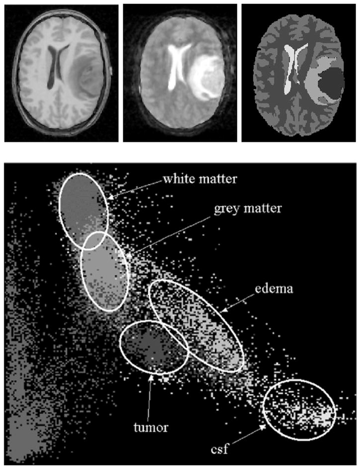
Top left: T1-weighted image. Top middle: T2-weighted image. Top right: labels from manual segmentation. Bottom: scatterplot of the T1 and T2 intensity features for Tumor020 based on the manual segmentation labels. The horizontal axis represents T2 intensities and the vertical axis represents T1 intensities.

Results

We have applied our automatic segmentation method to five tumor cases. The tool classifies the whole brain into healthy and pathological regions as shown in Figure 9. The validation of the method is done with the tumor volumes. For each case, we have two sets of manual segmentations, the second one done by the same rater more than three months after the first. The first set of manual segmentations is chosen as a gold standard for the purpose of evaluating the method. As another measure of performance, we also compared the manual segmentation results with the segmentations generated by a semi-automatic segmentation tool that uses level-set evolution (19). The semi-automatic segmentations are generated from the T1 contrast difference image with the user specifying the rough estimate of the tumor location by placing bubbles in the 3D volume. The tool uses this contrast difference image as a foreground/background probability and evolves a smooth surface capturing the tumor boundary. The volumes of the tumor structures for each case are shown in Table 1.

Figure 9.

Automatic segmentation result for the Tumor020 data. Left: T1 post-contrast image (for reference). Middle: Labels generated by the automatic method. Right: 3D view of the segmented tumor structure and cortical surface.

Table 1.

The volumes of the segmented tumor structure generated using different methods, measured in mm³.

Case	Manual 1	Manual 2	Semi-automatic	Automatic
Tumor020	35578.6	35114.5	33436.2	43052.3
Tumor022	24290.8	25215.8	22342.6	27305.6
Tumor025	24742.4	27802	26093.6	45800.4
Tumor031	72503	76842	65881	67907
Tumor032	56262.3	56807.4	47984.9	41925.3

The software used for the evaluation is VALMET (20). VALMET is used to generate two different classes of metrics for comparing two segmentations. The first metric class measures the volume of overlap between the two segmentations. The second metric class computes distances between the surfaces of the segmented structures. Two overlap measures are used. The first compares the volume of intersection with the combined volume, $\frac{(A\cap B)}{(A\cup B)}$. The second compares the volume of intersection with the first volume, $\frac{(A\cap B)}{A}$. If we treat the first segmentation as the gold standard, the second overlap measure ignores the false positives in segmentation B. Both overlap measures have a range of values between 0 (complete disagreement) and 1 (complete agreement). The surface distances used for this evaluation are the average surface distances with inward and outward direction (relative to the first segmented object), the average surface distance (absolute, both inward and outward), and the median surface distance.

The reliability of the manual segmentations is shown in Table 2. For all five cases, there is high degree of overlap and only 1 mm or less average surface distance. Thus, the intra-rater reliability of the manual segmentations is high. Table 3 shows the comparison between the manual segmentation results and the results generated by the semi-automatic level-set evolution tool. The resulting volumes tend to be smaller than manual segmentation volumes, which is reflected in the lower overlap measures and larger surface distance measures. Table 1 also indicates this fact. As shown in Table 4, the performance of the automatic method is consistently below that of the semi-automatic method. However, the automatic segmentation method has the advantage that it has no requirement of user interaction. For the first three of the five cases, the relatively low performance appears to be mainly caused by the number of false positives that the algorithm generates. For visual inspection, we have generated both the 2D and 3D views of the segmented structures generated by the automatic algorithm for the Tumor020 data (Figure 9). On average, the unsupervised segmentation process for one dataset takes 1 hour and 40 minutes on a 2GHz Intel Xeon machine. The user time required for setting up the segmentation parameters is normally less than 5 minutes.

Table 2.

A list of metrics comparing the two segmentations from the same human rater, which shows the intra-rater variability for each case. The second set of segmentations is done following the first set after a period of more than three months. All distances are in millimeters.

Case	Overlap 1	Overlap 2	Average Dist In	Average Dist Out	Average Distance	Median Distance
Tumor020	0.89	0.936	0.32	1.17	0.53	0
Tumor022	0.828	0.923	0.34	1.21	0.73	0.89
Tumor025	0.812	0.952	0.21	1.31	0.73	0.89
Tumor031	0.827	0.932	0.64	1.66	1.16	1.00
Tumor032	0.881	0.941	0.26	1.39	0.54	0

Table 3.

A list of metrics comparing the first set of manual segmentations and the results generated using the semi-automatic level-set evolution method. All distances are in millimeters.

Case	Overlap 1	Overlap 2	Average Dist In	Average Dist Out	Average Distance	Median Distance
Tumor020	0.873	0.904	0.47	1.13	0.60	0
Tumor022	0.85	0.882	0.34	1.01	0.47	0
Tumor025	0.763	0.889	0.57	1.42	0.89	0.89
Tumor031	0.813	0.856	1.13	1.63	1.27	1.00
Tumor032	0.789	0.817	1.39	1.40	1.39	0.86

Table 4.

A list of metrics comparing the first set of manual segmentations and the results of the automatic segmentation method. All distances are in millimeters.

Case	Overlap 1	Overlap 2	Average Dist In	Average Dist Out	Average Distance	Median Distance
Tumor020	0.71	0.918	1.92	2.54	2.25	1.77
Tumor022	0.57	0.771	1.69	3.29	2.59	2.01
Tumor025	0.49	0.937	1.28	4.94	4.21	3.24
Tumor031	0.586	0.716	3.79	3.25	3.57	2.83
Tumor032	0.578	0.639	3.59	3.52	3.56	3.0

Discussion

Conclusion

We have developed a model-based segmentation method for segmenting head MR image datasets with tumors and infiltrating edema. This is achieved by extending the spatial prior of a statistical normal human brain atlas with individual information derived from the patient’s dataset. Thus, we combine the statistical geometric prior with image-specific information for both geometry of newly appearing objects, and probability density functions for healthy tissue and pathology. Applications to five tumor patients with variable tumor appearance demonstrated that the procedure could handle large variation of tumor size, interior texture, and locality. The automatic procedure was compared to tumor segmentation by manual outlining and by using semi-automated level-set evolution tool. However, the significant benefits are increased efficiency and the segmentation of the whole brain structure including healthy tissue, tumor, and edema. Embedding tumor and edema into the proper three-dimensional anatomical context is crucial for planning, intervention, and monitoring.

The automatic method has a lower level of agreement with the human experts compared to the semi-automatic method. However, it generates a fully reproducible whole brain segmentation with embedded pathology and requires a lower degree of user supervision. The full brain segmentation provides anatomical context that may help in therapy planning and detecting deviation from normal. The clinical consequences of the lower level of agreement with the manual raters cannot be fully explored due to the limited number of cases. The results have been used in the analysis of vessel attributes in tumor volumes (21, 22). Compared to the results obtained with manual tumor segmentations, we observed no significant difference.

The lower agreement with the manual rater can be explained in terms of the underlying model. This method does voxel-by-voxel classification as opposed to a human rater who uses high-level human vision coupled with specialized domain knowledge. Discrimination by voxel intensities and the simplified geometric model for tumor shape cannot cope with tumors that have complex appearance and ambiguous boundaries. Furthermore, the lack of a true gold standard for healthy tissue and tumor is an inherent problem for validation.

In our future work, we will study the issue of deformation of normal anatomy in the presence of space-occupying tumors. Within the range of tumors studied so far, the soft boundaries of the statistical atlas (Figure 2) could handle spatial deformation. However, we will develop a scheme for high dimensional warping of multichannel probability data to get a better match between atlas and deformed patient images.

The VALMET validation software and the SNAP level-set evolution segmentation software are available for free download through the MIDAG homepage: http://midag.cs.unc.edu.

References

- 1.Just M, Thelen M. Tissue characterization with T1, T2, and proton density values: Results in 160 patients with brain tumors. Radiology. 1988;2:779–785. doi: 10.1148/radiology.169.3.3187000. [DOI] [PubMed] [Google Scholar]
- 2.Gerig G, Martin J, Kikinis R, Kubler O, Shenton M, Jolesz F. Automating segmentation of dual-echo MR head data. In: Colchester A, Hawkes D, editors. Proc IPMI 1991 LNCS 511. 1991. pp. 175–185. [Google Scholar]
- 3.Velthuizen R, Clarke L, Phuphianich S, Hall L, Bensaid A, Arrington J, Greenberg H, Siblinger M. Unsupervised measurement of brain tumor volume on MR images. JMRI. 1995;4:594–605. doi: 10.1002/jmri.1880050520. [DOI] [PubMed] [Google Scholar]
- 4.Vinitski S, Gonzales C, Mohamed F, Iwanaga T, Knobler R, Khalili K, Mack J. Improved intracranial lesion characterization by tissue segmentation based on a 3D feature map. Mag Re Med. 1997;5:457–469. doi: 10.1002/mrm.1910370325. [DOI] [PubMed] [Google Scholar]
- 5.Kamber M, Shingal R, Collins D, Francis D, Evans A. Model-based, 3-D segmentation of multiple sclerosis lesions in magnetic resonance brain images. IEEE-TMI. 1995;6:442–453. doi: 10.1109/42.414608. [DOI] [PubMed] [Google Scholar]
- 6.Zijdenbos A, Forghani R, Evans A. Automatic quantification of MS lesions in 3D MRI brain data sets: Validation of INSECT. In: Wells W, Colchester A, Delp S, editors. Proc MICCAI 1998 LNCS 1496. 1998. pp. 439–448. [Google Scholar]
- 7.Vehkomaki T, Gerig G, Szekely G. A user-guided tool for efficient segmentation of medical image data. In: Troccas J, Grimson W, Mosges R, editors. Proc CVRMed-MRCAS 1997 LNCS 1205. 1997. pp. 685–694. [Google Scholar]
- 8.Gibbs P, Buckley D, Blackband S, Horsman A. Tumour volume determination from MR images by morphological segmentation. Phys Med Biol. 1996;13:2437–2446. doi: 10.1088/0031-9155/41/11/014. [DOI] [PubMed] [Google Scholar]
- 9.Kjaer L, Ring P, Thomson C, Henriksen O. Texture analysis in quantitative MR imaging: Tissue characterization of normal brain and intracranial tumors at 1.5 T. Acta Radiologic. 1995;36:127–135. [PubMed] [Google Scholar]
- 10.Warfield S, Dengler J, Zaers J, Guttman C, Wells W, Ettinger G, Hiller J, Kikinis R. Automatic identification of gray matter structures from MRI to improve the segmentation of white matter lesions. J Image Guid Surg. 1995;1:326–338. doi: 10.1002/(SICI)1522-712X(1995)1:6<326::AID-IGS4>3.0.CO;2-C. [DOI] [PubMed] [Google Scholar]
- 11.Warfield S, Kaus M, Jolesz F, Kikinis R. Adaptive template moderated spatially varying statistical classification. In: Wells W, Colchester A, Delp S, editors. Proc MICCAI 1998 Springer LNCS 1496. 1998. pp. 431–438. [Google Scholar]
- 12.Wells W, Kikinis R, Grimson W, Jolesz F. Adaptive segmentation of MRI data. IEEE TMI. 1996;18:429–442. doi: 10.1109/42.511747. [DOI] [PubMed] [Google Scholar]
- 13.Van Leemput K, Maes F, Vandermeulen D, Suetens P. Automated model based tissue classification of MR images of the brain. IEEE TMI. 1999;18:897–908. doi: 10.1109/42.811270. [DOI] [PubMed] [Google Scholar]
- 14.Van Leemput K, Maes F, Vandermeulen D, Suetens P. Automated model based bias field correction of MR images of the brain. IEEE TMI. 1999;18:885–896. doi: 10.1109/42.811268. [DOI] [PubMed] [Google Scholar]
- 15.Van Leemput K, Maes F, Vandermeulen D, Colchester A, Suetens P. Automated segmentation of multiple sclerosis lesions by model outlier detection. IEEE TMI. 2001;20:677–688. doi: 10.1109/42.938237. [DOI] [PubMed] [Google Scholar]
- 16.Moon N, Bullitt E, Van Leemput K, Gerig G. Automatic brain and tumor segmentation. In: Dohi T, Kikinis R, editors. Proc MICCAI 2002 Springer LNCS 2488. 2002. pp. 372–379. [Google Scholar]
- 17.Evans A, Collins D, Mills S, Brown E, Kelly R, Peters T. 3D statistical neuroanatomical models from 305 MRI volumes. Proc IEEE Nuclear Science Symposium and Medical Imaging Conference; 1993. pp. 1813–1817. [Google Scholar]
- 18.Maes F, Collignon A, Vandermeulen D, Marchal G, Suetens P. Multimodality image registration by maximization of mutual information. IEEE TMI. 1997;16:187–198. doi: 10.1109/42.563664. [DOI] [PubMed] [Google Scholar]
- 19.Ho S, Bullitt E, Gerig G. Level set evolution with region competition: automatic 3-D segmentation of brain tumors. In: Katsuri R, Laurendeau D, Suen C, editors. Proc. 16th Int Conf on Pattern Recognition ICPR; 2002. pp. 532–535. [Google Scholar]
- 20.Gerig G, Jomier M, Chakos M. VALMET: A new validation tool for assessing and improving 3D object segmentation. In: Niessen W, Viergever M, editors. Proc MICCAI 2001 Springer LLNCS 2208; 2001. pp. 516–523. [Google Scholar]
- 21.Bullitt E, Gerig G, Pizer SM, Aylward SR. Measuring tortuosity of the intracerebral vasculature from MRA images. IEEE-TMI 2003. doi: 10.1109/TMI.2003.816964. To appear September 2003. [DOI] [PMC free article] [PubMed] [Google Scholar]
- 22.Bullitt E, Gerig G, Aylward S, Joshi S, Smith K, Ewend M, Lin W. Vascular attributes and malignant brain tumors. In: Ellis R, Peters T, editors. Proc MICCAI 2003 Springler LNCS. To appear November 2003. [Google Scholar]