A New Pattern Electroretinogram Paradigm Evaluated in Terms of User Friendliness and Agreement with Perimetry

Abstract

Purpose

To assess ease of use of the pattern electroretinogram optimized for glaucoma screening (PERGLA) paradigm by a novice operator; to study test–retest variability of the PERGLA parameters; and to compare results from the PERGLA to those from perimetry.

Design

Cohort study.

Participants

Twelve healthy control subjects and 16 patients with moderate to advanced glaucoma in at least 1 eye.

Methods

Pattern electroretinograms were recorded simultaneously from both eyes using a commercially available testing station. Each participant underwent PERGLA procedures in 2 sessions. One eye of each subject was tested on contrast sensitivity perimetry (CSP) in which a 0.4 cycles/degree Gabor patch served as a stimulus. Central visual fields results from conventional automated perimetry (CAP) were obtained from patients’ records. Bland–Altman analysis was performed on PERGLA results to assess normal test–retest variability. Differences from mean normal (in decibels [dB]) were compared for PERGLA versus CSP and CAP.

Main Outcome Measures

Pattern electroretinogram amplitude, noise, phase, and test–retest variability (coefficient of variation); contrast sensitivity from CSP; perimetric sensitivity from CAP; and differences from mean normal for PERGLA, CSP, and CAP.

Results

The mean log amplitude (0.08±0.12 log μV) and the mean phase (1.92±0.07 π rad) for the control group were consistent with published PERGLA norms, as was test–retest variability for both amplitude (coefficient of variation [CV] = 8.2±7.0%) and phase (CV = 1.1±0.9%). The mean signal-to-noise ratio (8.7±4.5) was lower than published norms. The test–retest variability increased as PERGLA log amplitude decreased (R²>0.12, P<0.05). On average, differences from mean normal were similar for PERGLA versus CSP and for PERGLA versus CAP (mean differences<0.5 dB) with 95% confidence intervals near ±4 dB in both comparisons.

Conclusions

A novice operator successfully replicated published PERGLA norms in a young control group for amplitude, phase, and repeatability. Higher test–retest variability was found in eyes with smaller signals. On average, PERGLA results were in reasonable agreement with those from perimetry, although there existed large individual differences which may limit the usage of PERGLA in screening or in following progression of glaucoma.

The pattern electroretinograms (PERGs) have been shown to reflect retinal ganglion cell function in experimental glaucoma.¹ Clinical researchers have found that patients with glaucomatous damage can have significant decreases in PERG amplitude.^2–5 However, the PERG has not been used widely because its signal is relatively small, and traditional PERG recording procedures are rather complex, requiring highly experienced operators and usage of corneal electrodes.

Perimetry, by comparison, is widely utilized in the field of glaucoma, but has its own shortcomings, such as a learning curve and effect of fatigue of a test taker, and variability in individuals’ subjective responses. Compared with perimetry, which measures visual function subjectively using a threshold stimulus, the PERG measures visual function objectively using a suprathreshold stimulus, eliminating some of the challenges inherent to a psychophysical test. The PERG can detect early glaucomatous defects when the conventional perimetry does not show significant defects.^2,3 If the complex nature of PERG recording procedures can be improved, then the PERG would have the potential to become a clinically useful method for detecting losses in visual function caused by glaucoma.

Porciatti and Ventura have introduced a new testing paradigm, the PERG optimized for glaucoma screening (PERGLA),⁶ which is designed to be user friendly and obtain rapid measurements with automated analysis. They also have provided normative data across a wide range of ages. In the current study, a novice operator with minimal training in electrophysiology explored the PERGLA testing paradigm.

In the first part of the present study, a novice operator attempted to replicate norms in young healthy individuals. Second, we investigated test–retest variability of the PERGLA to see whether it increases with difference from mean normal as it does in perimetry.^7–9 In addition, PERGLA results were directly compared to results from 2 types of perimetry, contrast sensitivity perimetry (CSP)¹⁰ and conventional automated perimetry (CAP).

Materials and Methods

Subjects

Control subjects were recruited from the student body at the State University of New York, State College of Optometry. Inclusion criteria were (1) age 22 to 28 years, (2) best-corrected visual acuity of at least 20/20 in each eye, (3) no ocular disease on comprehensive eye examination within 2 years, (4) no systemic disease or medications known to affect visual function, (5) spherical correction within ± 3.50 diopters, (6) cylindrical correction within −2.00 diopters, and (7) clear ocular media. Twelve volunteers, ages ranging from 22 to 28 years, participated. When measured on the first day of testing, all 12 subjects had Snellen visual acuity of at least 20/20 in each eye and a Pelli-Robson contrast sensitivity score of at least 1.65 in each eye. When optimally corrected for the near viewing distance of PERGLA and CSP, all control subjects denied experiencing accommodative fluctuation during the test.

The inclusion criteria for subjects with glaucoma were (1) age ≥ 22 years, (2) best-corrected visual acuity of at least 20/30 in the better eye on the day of testing, (3) moderate to advanced glaucoma in at least one eye, (4) no other eye disease, (5) no systemic disease or medications known to affect visual function, (6) pupil size ≥2 mm, (7) spherical correction within ± 3.50 diopters, (8) cylindrical correction within −2.00 diopters, and (9) no more than mild lens changes. Sixteen patients (9 males and 7 females), ages 44 to 70 years, from the Glaucoma Institute at the State College of Optometry participated in this study. Diagnosis of glaucoma was based on the following criteria: optic disc changes consistent with glaucoma, pre-treated intraocular pressure > 25 mmHg, and pattern of visual field loss characteristic of glaucoma. The diagnosis was reviewed and confirmed by one of the authors (AY), and patients with moderate to advanced glaucoma (mean deviation on central 24 or 30 degrees automated perimetry worse than −6.00 decibels [dB]) were included. As assessed in the most recent glaucoma follow-up visits within 3 months, no patient had other ocular disease besides glaucoma. All patients had either no or minimal lens changes, or clear posterior capsule after uncomplicated cataract extraction. All patients were experienced with conventional perimetry and demonstrated adequate fixation and reliability. Table 1 describes further characteristics of patients.

Table 1.

Characteristics of Patients with Glaucoma (n = 16) (Sorted in an Increasing Order of the Visual Field Mean Deviation of the Left Eye)

		Visual Acuity				Visual Field
		logMAR		Contrast Sensitivity*		MD		PSD
Age	Gender	Right	Left	Right	Left	Right	Left	Right	Left
63	F	0.12	0.02	1.50	1.50	−9.91	−0.29	12.58	2.00
61	F	0.06	0.06	1.50	1.50	−12.41	−1.08	13.89	1.33
54	F	0.20	0.24	1.20	1.35	−16.67	−1.30	12.15	1.66
68	M	−0.04	−0.08	1.35	1.60	−5.46	−2.34	7.08	4.50
58	F	0.02	−0.02	1.35	1.65	−0.52	−2.43	3.13	2.14
44	F	0.00	−0.10	1.50	1.50	−10.68	−3.01	13.33	8.18
61	M	0.24	0.12	1.20	1.35	−5.30	−3.25	3.00	2.35
60	F	0.24	0.34	1.05	0.95	−17.77	−6.02	12.34	5.28
60	F	0.12	0.00	1.65	1.50	−2.61	−6.16	5.06	4.65
55	M	0.06	0.06	1.55	1.55	−8.73	−6.20	7.33	3.46
55	M	0.06	0.14	1.05	1.05	−6.68	−6.36	9.33	6.34
58	M	0.04	−0.10	1.65	1.65	0.05	−6.37	1.77	8.88
44	M	−0.10	−0.08	1.50	1.55	−3.32	−8.97	5.85	8.27
69	M	0.08	0.04	1.35	1.20	−0.75	−10.17	2.08	12.26
68	M	0.10	0.16	1.25	1.20	−8.85	−12.91	13.63	15.43
49	M	NLP	0.08	NLP	1.50	−25.25†	−27.06	11.69†	12.02

F = female; logMAR = logarithm of the minimum angle of resolution; M = male; MD = mean deviation; PSD = pattern standard deviation; NLP = no light perception.

^*Contrast sensitivity was measured with the Pelli-Robson chart.

^†MD and PSD of the NLP eye were obtained from the most recent visual field prior to becoming NLP.

After explaining the protocol for the study and answering any questions, written informed consent was obtained from each subject before testing. The study was compliant with the Health Insurance Portability and Accountability Act and was approved by the institutional review board of State University of New York, State College of Optometry.

Equipment

The PERGs were recorded using a commercial device called “Glaid” (Lace Elettronica, Pisa, Italy), as described by Porciatti and Ventura.⁶ The stimulus consisted of a horizontal black and white square-wave grating, which was displayed on a circular screen, housed in a Ganzfeld bowl at a viewing distance of 30 cm, covering 25 degrees diameter in visual angle. The mean luminance of the stimulus was 40 candelas/m², and the spatial frequency of the grating was 1.6 cycles/degree, reversing in counterphase at 8.14 Hz with 98% contrast. Five gold skin electrodes taped to the subject’s face were connected to a preamplifier connection box, which fed signals to an amplifier. Amplified and digitally converted signals were displayed on a computer monitor. The impedance of electrodes was monitored automatically with an indicator on the monitor.

The CSP stimulus consisted of a Gabor sine-wave patch with a peak spatial frequency of 0.375 cycles/degree and a spatial band width of 1.5 octaves (Fig 1). To avoid sharp edges and maintain a constant mean luminance of the patch, a Gaussian envelope was used in sine phase. The Gabor patch was approximately 4 degrees in size when displayed on a flat computer screen and viewed from 40 cm. The temporal presentation of the stimulus was Gaussian as well, with the majority of the energy presenting within 200 milliseconds. The Gabor stimulus was presented at 26 locations in the visual field (gray background with luminance of 50 candelas/m²) at different levels of contrast. These 26 locations corresponded to approximately one half of the points in a 24-2 Humphrey visual field, with extra points in the nasal hemifield and fewer points in the temporal hemifield.

Figure 1.

Stimuli used in this study are shown side by side. Left, A size III stimulus for conventional automated perimetry (CAP). Middle, A portion of the 25-degree radius PERGLA (pattern electroretinogram optimized for glaucoma screening) stimulus. Right, The Gabor stimulus for contrast sensitivity perimetry (CSP).

Conventional automated perimetry tests were conducted on the Humphrey Field Analyzer 750i (Carl Zeiss Meditec, Jena, Germany), using the Swedish Interactive Thresholding Algorithm Standard with size III (0.43-degree visual angle) stimulus in rectangular spatial and temporal profiles presented for 200 milliseconds.

Procedures

Pattern Electroretinogram

Small patches of skin (central forehead, both temples, and 5 mm below each lower eyelid margin) were cleaned with alcohol pads (30–40 rubs at each location). Five gold skin electrodes filled with conductive paste were firmly taped to the cleaned skin areas using micropore tapes. The test was conducted without any ambient or extraneous lighting in the room. The PERGs were recorded from both eyes simultaneously while the subjects were viewing the stimulus through age-appropriate corrective lenses for the near viewing distance (30 cm). Subjects were told to blink naturally while fixating at the center of the stimulus. The electrical signals from large eye movements such as blinking were automatically rejected. After obtaining a steady-state response from the first block of 300 acceptable sweeps, subjects were allowed to rest for 1 minute before recording the second block of 300 sweeps. The sinusoidal responses from the two 300 sweeps were averaged, and the average amplitude and phase were plotted on a polar diagram along with the age-predicted normal ranges. Each subject (total of 12 controls and 16 patients) was tested in 2 sessions, the first test (Test₁) and the second test (Test₂) at least 2 days and no more than 14 days apart.

Contrast Sensitivity Perimetry

All 12 control subjects and 15 of the 16 patients performed CSP. Only 1 eye (randomly chosen) of each control subject was tested. For patients, an eye with more severe glaucoma was chosen for the test as long as the eye had 20/30 or better central visual acuity. Subjects were instructed to fixate a cross at the center of the computer screen at all times, and to press a mouse button each time a Gabor stimulus was seen in the periphery. The procedure was similar to CAP. Fixation was monitored by the Heijl–Krakau blind spot monitoring technique using a smaller Gabor patch at 100% contrast. The operator also monitored the subject’s fixation visually through a video camera. The false-positive rate was checked by presenting a blank stimulus and recording incorrect responses. The false-negative rate was calculated using maximum likelihood estimation.¹¹ Data from only 1 control subject were excluded from the analysis, owing to false-positive responses exceeding 25%.

Conventional Automated Perimetry

For patients, we gathered the most recent clinical visual field results from the Humphrey field analyzer. Visual field tests obtained within 4 months of the PERGLA test were included for analysis. Fourteen right eye and 14 left eye visual fields of the 16 patients met this time criterion. All patients had taken either 24-2 or 30-2 Swedish Interactive Thresholding Algorithm Standard visual field tests. When 10-2 Swedish Interactive Thresholding Algorithm Standard visual field results were also available, we used 10-2 results instead of 24-2 or 30-2. There were two 10-2 fields for the right eye and one 10-2 field for the left eye.

Statistical Design

We analyzed each eye of control subjects separately and used the results from the left eyes only for comparison with published PERGLA norms.⁶ To compare our means with published norms, we computed Z scores for the difference between our means and the norms, using our standard error of the mean (SEM; Z = difference of means ÷ SEM; SEM = standard deviation (SD) ÷ √ [n–1]). Amplitude was analyzed in log units and phase was analyzed in linear units as in the previous study.⁶ Because coefficient of variation (CV = [SD ÷ Mean] × 100) was used to describe within-subject variability in the previous study, we calculated mean CV, using linear units for amplitude and phase. An F-test (SD in log units) was performed to compare our between-subject variability with the norms.

We employed Bland–Altman analysis^12,13 where the difference between Test₁ and Test₂ was plotted against the mean of the 2 values, in log units for PERGLA amplitude and in linear units for PERGLA phase. The Bland–Altman analysis helps to identify learning effects or other systematic changes from one test to the next. In this analysis, we adopted the approach that is commonly used in perimetry for test–retest variability, rather than looking for more precise measurement in the retest. The Pearson correlation coefficient (R) was computed from the mean and the difference between Test₁ and Test₂. Because we analyzed the right and left eyes separately, we reported R² values with limits; that is, we reported “R² <” a number 1 significant figure greater than the larger of the 2 (if both were not significant) or “R² >” a number 1 significant figure smaller than the smaller of the 2 (if both were significant). The mean difference and the 95% confidence intervals were computed, based on a Gaussian distribution. To assess whether test–retest variability was dependent on the mean, we studied the relation between the absolute difference of the 2 amplitude values and the mean of the 2. For this purpose, data from the controls and the patients were combined, and the analysis was performed in both log and linear units. An F-test was performed to compare test–retest SD between 2 subgroups of patients: one subgroup with mean amplitude ≤ 0.5 μV and the other subgroup with mean amplitude > 0.5 μV.

To compare the PERGLA with CSP, the contrast sensitivity values from the central 8 test locations in CSP, which corresponded to the area tested by the PERGLA stimulus, were averaged into one arithmetic mean^4,14 and then converted to log units. The mean PERGLA results were expressed in log amplitude. Because contrast sensitivity and PERGLA amplitude were measures of 2 different entities, relative losses for each parameter compared with its own mean normal were used to compare the PERGLA to CSP. To illustrate the results in clinically familiar units, a decibel scale was used (10 dB = 1 log unit).

The same statistical methods were applied to compare the PERGLA to CAP. The threshold decibel values from the central 16 test locations in CAP (or all locations when a 10-2 field was available) were first converted into linear units and then averaged. This arithmetic mean was, in turn, converted to log and decibel units. The relative losses for CAP were computed using Heijl’s norms.¹⁵

Results

Table 2 summarizes mean PERGLA results obtained from the control group. Our mean amplitude was very similar to the published norm (Z<0.001, P>0.91), and the mean phase was identical to the norm. For our sample size of 12, we calculated that mean differences of 0.10 log μV and 0.06 π rad (≈ 3.7 msec) could be detected at significance level of 0.05 with a power of 0.80. Within-subject variability expressed in mean CV was identical to the norms for amplitude and very similar for phase. Between-subject variabilities for amplitude and phase were also similar to the norms (F_amp = 1.3, P>0.23; F_phase = 1.5, P>0.14).

Table 2.

Mean PERGLA (Pattern Electroretinogram Optimized for Glaucoma Screening) Results for Control Subjects (n = 12)

	Amplitude		Phase
Eye	Mean of T1 and T2 (log μV)	Test-Retest Variability CV (%)	Mean of T1 and T2 (π rad)	Test–Retest Variability CV (%)
Right	0.06±0.12	14.0±13.9	1.93±0.06 (≈ 118.6 msec)	1.3±1.0
Left	0.08±0.12	8.2±7.0	1.92±0.07 (≈ 117.9 msec)	1.1±0.9

CV = coefficient of variation; T₁ = first test; T₂ = second test.

Figure 2 shows simple scatterplots of Test₂ versus Test₁ for amplitude and phase, and Figure 3 illustrates the results of Bland– Altman analysis of test–retest differences for the PERGLA. The mean amplitude difference between Test₁ and Test₂ was less than −0.03 (±0.12 SD) log μV in the control group and less than −0.06 (±0.15 SD) log μV in the patient group. The mean phase difference was about +0.01 (±0.05 SD) π rad (≈ 0.6 msec) and less than +0.06 (±0.16 SD) π rad (≈ 3.7 msec) in the control and patient groups, respectively. There was a significant dependence of the amplitude intertest variability on the mean amplitude in the control group (R²>0.41, P<0.02). The phase variability in the control group (R²<0.15, P>0.10) and both amplitude and phase variabilities in the patient group were not dependent on their respective means (R²<0.07, P>0.20). The absolute test–retest variability for amplitude increased as the mean log amplitude decreased (R²>0.12, P<0.05; Fig 4, right). However, when amplitude was expressed in linear units (μV), the correlation was weaker (R²<0.04, P>0.20; Fig 4, left). The test–retest SD for patients with smaller amplitudes was significantly larger than for patients with larger amplitudes when the amplitudes were analyzed in log units (F>4, P<0.05). In linear units, the test–retest SD was not significantly different between these 2 subgroups of patients (F ≈ 1.1, P>0.50). The absolute test–retest variability for phase was not dependent on the mean phase in either log units (R²<0.01, P>0.50) or linear units (R²<0.006, P>0.50).

Figure 2.

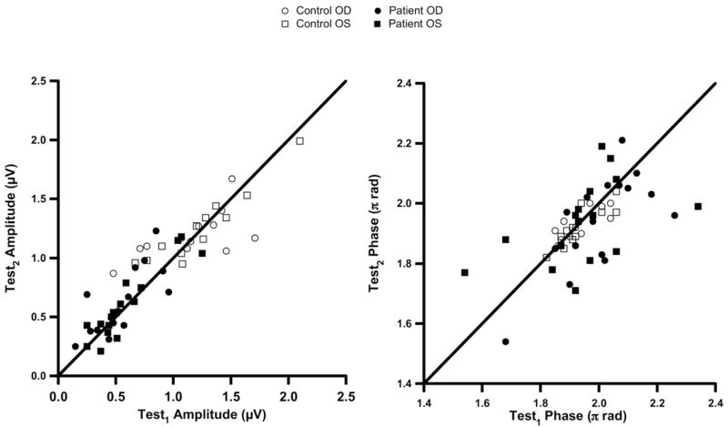
Scatterplots of Test₂ (the second test) versus Test₁ (the first test) for PERGLA (pattern electroretinogram optimized for glaucoma screening) amplitude (left) and phase (right). The diagonal lines show equality. μV = microvolts; OD = right eye; OS = left eye

Figure 3.

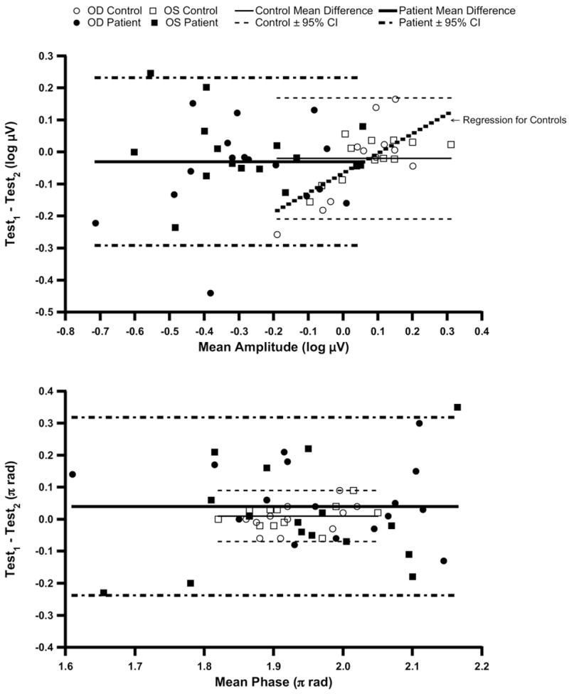
Bland–Altman analysis of PERGLA (pattern electroretinogram optimized for glaucoma screening) test–retest agreement: amplitude test–retest differences against mean amplitudes in log units (top) and phase test–retest differences against mean phases in linear units (bottom). The solid horizontal lines indicate mean difference and the dashed lines indicate 95% confidence intervals (CIs). μV = microvolts; OD = right eye; OS = left eye.

Figure 4.

Plots of test–retest variability versus PERGLA (pattern electroretinogram optimized for glaucoma screening) mean amplitudes in linear units (left) and in log units (right). μV = microvolts; OD = right eye; OS = left eye.

Contrast sensitivity perimetry versus PERGLA results are depicted in Figure 5 (left) as a scatterplot in linear units. Figure 5 (right) also shows relative losses (in decibel scale) for each measure (compared to mean normal) in a scatterplot. On average, the difference from mean normal was similar for the 2 tests (mean difference < 1 dB for both patient and control groups) with 95% confidence intervals of ±3.1 dB for the control group and ±3.9 dB for the patient group (excluding one outlier with −6.5 dB for PERGLA and −11.5 dB for CSP). The agreement between PERGLA and CSP was independent of their average difference from mean normal (controls, R²<0.12, P>0.20; patients, R² = 0.001, P>0.50). Figure 6 (left) shows a scatterplot of CAP versus PERGLA amplitude in linear units. On average, the difference from mean normal was similar for the 2 tests (mean difference of −0.3 dB) with 95% confidence intervals of ± 4.5 dB (Fig 6, right). The agreement between PERGLA and CAP was independent of their average difference from mean normal (R²<0.04, P>0.20).

Figure 5.

Plots of contrast sensitivities from CSP (contrast sensitivity perimetry) versus PERGLA (pattern electroretinogram optimized for glaucoma screening) amplitudes in linear units (left) and in log units (right). The arrows on the x-axis indicate PERGLA amplitude and corresponding relative loss (decibels [dB]) in an eye with no light perception. The mean and its 95% confidence intervals (CIs) (for the patient group only) from Bland–Altman analysis are shown as diagonal lines in both scales. For the Bland–Altman analysis, an outlier with PERGLA loss of −6.5 dB and CSP loss of −11.5 dB was excluded. μV = microvolts.

Figure 6.

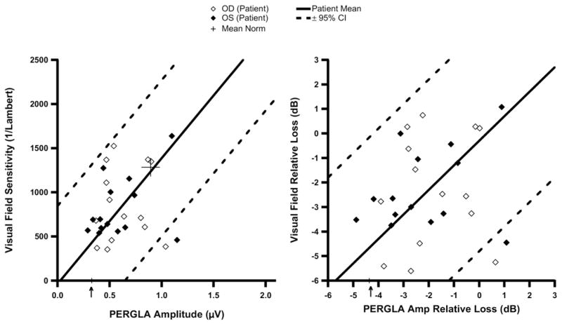
Plots of central visual field sensitivities from conventional automated perimetry (CAP) versus PERGLA (pattern electroretinogram optimized for glaucoma screening) amplitudes in linear units (left) and in log units (right). The arrows on the x-axis indicate PERGLA amplitude and corresponding relative loss (decibels [dB]) in an eye with no light perception. The mean and its 95% confidence intervals (CIs) from Bland–Altman analysis are shown as diagonal lines in both scales. μV = microvolts; OD = right eye; OS = left eye.

Discussion

The primary purpose of this study was to explore the new testing paradigm, the PERGLA, for its patient and operator friendliness. Our novice operator found that the PERGLA was relatively simple to operate and its automated output easy to obtain. Patients’ high acceptance was aided by short testing duration (4–5 minutes) and no need for corneal anesthesia. In the first part of this study, we successfully replicated PERGLA norms established by Porciatti and Ventura.⁶ The mean amplitude and phase, and their respective SDs were consistent with published norms. Test–retest variability expressed in mean coefficient of variation was 11% for amplitude and 1.2% for phase (all control eyes combined). These values were comparable to PERGLA norms; they were also consistent with typical reproducibility in electrophysiology.¹⁶

To study the potential effects of the operator’s learning curve on the PERGLA results, all control subjects were tested before the patients. Among the control subjects (all eyes combined), the mean difference between Test₁ and Test₂ was −0.03 μV for amplitude and +0.01 π rad (≈ 0.6 msec) for phase, indicating on average a minimal effect of the operator’s learning curve. However, for the control group the amplitude difference between the 2 tests was dependent on the mean, with a positive slope indicating that those with the lowest mean amplitude had higher amplitudes on retests. This could be an indication of an effect of operator’s learning curve.

The SD of differences between tests was <1 dB for amplitude and 0.1 dB for phase, when expressed in the units commonly used in standard automated perimetry. The amplitude variability was larger and the phase variability was similar when compared with the results found in a recent study by Ventura and Porciatti.¹⁷ Such a difference in amplitude variability may be due to the fact that our comparison was performed on logarithmic scale, which magnifies effects at smaller amplitudes.

Although we were able to replicate the published norms for mean amplitude and phase, our mean signal-to-noise ratio (SNR) was 8.7±4.5 compared with the published value of 13.7. This was mainly due to a higher noise level (mean = 0.16±0.06 μV), perhaps resulting from a higher level of electrode impedance in the present study performed by the inexperienced operator. Variation in electrode impedance may also account for the evidence of an operator learning curve in the control group, which was tested first. With a smaller SNR, the dynamic range for PERGLA amplitude would be narrower, making it difficult to differentiate true signals from noise when the signals are small.

The analysis of the combined PERGLA data from the control subjects and the patients found that test–retest variability increased with difference from mean normal. This was similar to already established findings in perimetry.^7–9 However, this dependence was observed only when PERGLA amplitudes were expressed in log units, and not in linear units. A separate analysis for the patient group also showed similar results. Because there has not been any assessment of test–retest variability for perimetry in linear units, the significance of our finding is yet to be determined. To compare the magnitude of the PERGLA’s intertest variability to that of perimetry, a study with a larger sample size would be required.

Clinicians need to be cautious when interpreting PERGLA results if the amplitude is near the noise level. When the SNR, defined as measured amplitude divided by measured noise, is <3, we considered it to be too small and flagged the data points for exclusion in a secondary analysis. None of the control subjects had such small SNR, but for half of the patients the measured SNR was <3 in at least 1 eye in 1 of the 2 repeated tests. When we repeated the analyses excluding these subjects, the dependence of the amplitude test–retest variability on the mean log amplitude became weaker in the left eye (R² = 0.05, P>0.20). Therefore, the initial observation of a negative correlation between the intertest variability and the mean amplitude of the 2 tests may be at least partially due to the eyes with amplitudes very close to the noise level.

One patient, who recently became “no light perception” in 1 eye from end-stage glaucoma, yielded a SNR of 4. This result is consistent with Hood et al’s observation that glaucomatous damage may not reduce PERG amplitude to noise level.⁵ They also pointed out that the wide range of normal PERG amplitudes resulted in some patients having normal PERG amplitudes despite clear visual field defects. There are others who found similar results.^4,18 Such findings suggest that the PERGLA paradigm may not be suitable for following patients with advanced loss from glaucoma.

Our sample size was not adequate to obtain a precise estimate of sensitivity and specificity of PERGLA abnormality for detecting glaucoma. For a rough estimate, we found that out of 25 eyes with definite (moderate to advanced) glaucoma, 17 eyes yielded PERGLA amplitudes below the 95% confidence limits (sensitivity of approximately 68% at a specificity of 97.5%). A lower sensitivity (<40%) was found by Ventura et al¹⁹ who tested patients with early manifest glaucoma. An earlier study by Graham et al²⁰ also reported a sensitivity < 40% at a specificity of 97.5% when the PERG amplitude was measured in patients with early glaucoma. Therefore, the PERG does not seem suitable for screening for early glaucomatous loss.

When the results from the PERGLA were compared with the averaged contrast sensitivities from the central locations covered by PERGLA stimulus, the mean difference in relative loss between PERGLA and CSP was <1 dB. However, there still existed substantial individual variations, yielding a 95% confidence interval of ±4.1 dB, compared with ±1.9 dB for the PERGLA’s intertest difference. The CAP measurements were available for the patients only. On average, the agreement between CAP and the PERGLA was similar to that between CSP and the PERGLA. These results are consistent with findings from the studies of Garway-Heath et al⁴ and Hood et al¹⁴ comparing results from electrophysiology and perimetry.

It has been suggested that the PERGLA, in which only the central 25 degrees of retina is stimulated, could be an indicator for a diffuse retinal ganglion cell dysfunction.¹⁷ When we repeated analyses where PERGLA results were compared to the averaged sensitivities from the entire field of each perimetric test (CSP and CAP), including areas outside the central 25 degrees, the results were similar to earlier analyses with central 25 degrees only; the differences from mean normal were similar (CSP averaged 1.3 dB farther below normal than PERGLA; PERGLA averaged 0.6 dB farther below normal than CAP) with a 95% confidence interval of ±4.1 dB in both comparisons. The underlying reason(s) for such similar results between these measures is not clear. Future studies addressing the question of the extent to which the PERG reflects diffuse retinal dysfunction may help us better understand the relations between PERGLA and perimetry.

In summary, our operator with minimal training in electrophysiology was able to obtain repeatable PERGLA results from healthy control subjects and patients with glaucoma after relatively short training. The short testing duration, no need for patients’ active participation, and no need for repeated baseline tests to overcome patients’ learning curves were found to be advantageous. We also learned that interpreting PERGLA results can be challenging due to (1) larger test–retest variability in eyes with reduced PERGLA amplitudes, (2) relatively small SNRs, and (3) normal PERGLA results from patients with obvious glaucoma and established visual field damage. Results from the PERGLA and perimetry were in good agreement on average, although not necessarily for individual patients. The PERGLA may offer an additional testing paradigm to the currently available armamentarium for evaluation of glaucomatous visual loss. The potential for the PERGLA is in clinical studies that evaluate averaged data and disease mechanisms, comparing groups of people tested with a variety of tools such as PERG, perimetry, and imaging technologies.

References

- 1.Viswanathan S, Frishman LJ, Robson JG. The uniform field and pattern ERG in macaques with experimental glaucoma: removal of spiking activity. Invest Ophthalmol Vis Sci. 2000;41:2797–810. [PubMed] [Google Scholar]
- 2.Korth M, Horn F, Storck B, Jonas J. The pattern-evoked electroretinogram (PERG): age-related alterations and changes in glaucoma. Graefes Arch Clin Exp Ophthalmol. 1989;227:123–30. doi: 10.1007/BF02169783. [DOI] [PubMed] [Google Scholar]
- 3.Bach M, Sulimma F, Gerling J. Little correlation of the pattern electroretinogram (PERG) and visual field measures in early glaucoma. Doc Ophthalmol. 1998;94:253–63. doi: 10.1007/BF02582983. [DOI] [PubMed] [Google Scholar]
- 4.Garway-Heath DF, Holder GE, Fitzke FW, Hitchings RA. Relationship between electrophysiological, psychophysical, and anatomical measurements in glaucoma. Invest Ophthalmol Vis Sci. 2002;43:2213–20. [PubMed] [Google Scholar]
- 5.Hood DC, Xu L, Thienprasiddhi P, et al. The pattern electroretinogram in glaucoma patients with confirmed visual field deficits. Invest Ophthalmol Vis Sci. 2005;46:2411–8. doi: 10.1167/iovs.05-0238. [DOI] [PubMed] [Google Scholar]
- 6.Porciatti V, Ventura LM. Normative data for a user-friendly paradigm for pattern electroretinogram recording. Ophthalmology. 2004;111:161–8. doi: 10.1016/j.ophtha.2003.04.007. [DOI] [PMC free article] [PubMed] [Google Scholar]
- 7.Heijl A, Lindgren A, Lindgren G. Test-retest variability in glaucomatous visual fields. Am J Ophthalmol. 1989;108:130–5. doi: 10.1016/0002-9394(89)90006-8. [DOI] [PubMed] [Google Scholar]
- 8.Piltz JR, Starita RJ. Test-retest variability in glaucomatous visual fields [letter] Am J Ophthalmol. 1990;109:109–11. [PubMed] [Google Scholar]
- 9.Henson DB, Chaudry S, Artes PH, et al. Response variability in the visual field: comparison of optic neuritis, glaucoma, ocular hypertension, and normal eyes. Invest Ophthalmol Vis Sci. 2000;41:417–21. [PubMed] [Google Scholar]
- 10.Harwerth RS, Crawford ML, Frishman LJ, et al. Visual field defects and neural losses from experimental glaucoma. Prog Retin Eye Res. 2002;21:91–125. doi: 10.1016/s1350-9462(01)00022-2. [DOI] [PubMed] [Google Scholar]
- 11.Swanson WH, Birch EE. Extracting thresholds from noisy psychophysical data. Percept Psychophys. 1992;51:409–22. doi: 10.3758/bf03211637. [DOI] [PubMed] [Google Scholar]
- 12.Bland JM, Altman DG. Statistical methods for assessing agreement between two methods of clinical measurement. Lancet. 1986;1:307–10. [PubMed] [Google Scholar]
- 13.Bland JM, Altman DG. Measurement error. BMJ. 1996;313:744. doi: 10.1136/bmj.313.7059.744. [DOI] [PMC free article] [PubMed] [Google Scholar]
- 14.Hood DC, Greenstein VC, Odel JG, et al. Visual field defects and multifocal visual evoked potentials: evidence of a linear relationship. Arch Ophthalmol. 2002;120:1672–81. doi: 10.1001/archopht.120.12.1672. [DOI] [PubMed] [Google Scholar]
- 15.Heijl A, Lindgren G, Olsson J. Normal variability of static perimetric threshold values across the central visual field. Arch Ophthalmol. 1987;105:1544–9. doi: 10.1001/archopht.1987.01060110090039. [DOI] [PubMed] [Google Scholar]
- 16.Otto T, Bach M. Retest variability and diurnal effects in the pattern electroretinogram. Doc Ophthalmol. 1996–1997;92:311–23. doi: 10.1007/BF02584085. [DOI] [PubMed] [Google Scholar]
- 17.Ventura LM, Porciatti V. Restoration of retinal ganglion cell function in early glaucoma after intraocular pressure reduction: a pilot study. Ophthalmology. 2005;112:20–7. doi: 10.1016/j.ophtha.2004.09.002. [DOI] [PMC free article] [PubMed] [Google Scholar]
- 18.Drasdo N, Aldebasi YH, Chiti Z, et al. The S-cone PHNR and pattern ERG in primary open angle glaucoma. Invest Ophthalmol Vis Sci. 2001;42:1266–72. [PubMed] [Google Scholar]
- 19.Ventura LM, Porciatti V, Ishida K, et al. Pattern electroretinogram abnormality and glaucoma. Ophthalmology. 2005;112:10–9. doi: 10.1016/j.ophtha.2004.07.018. [DOI] [PMC free article] [PubMed] [Google Scholar]
- 20.Graham SL, Drance SM, Chauhan BC, et al. Comparison of psychophysical and electrophysiological testing in early glaucoma. Invest Ophthalmol Vis Sci. 1996;37:2651–62. [PubMed] [Google Scholar]