

Abstract
Previous research provided evidence of an association between short-term exposure to ozone and mortality risk and of heterogeneity in the risk across communities. The authors investigated whether this heterogeneity can be explained by community-specific characteristics: race, income, education, urbanization, transportation use, particulate matter and ozone levels, number of ozone monitors, weather, and use of air conditioning. Their study included data on 98 US urban communities for 1987 to 2000 from the National Morbidity, Mortality, and Air Pollution Study; US Census; and American Housing Survey. On average across the communities, a 10-ppb increase in the previous week's ozone level was associated with a 0.52% (95% posterior interval: 0.28, 0.77) increase in mortality. The authors found that community-level characteristics modify the relation between ozone and mortality. Higher effect estimates were associated with higher unemployment, fraction of the Black/African-American population, and public transportation use and with lower temperatures or prevalence of central air conditioning. These differences may relate to underlying health status, differences in exposure, or other factors. Results show that some segments of the population may face higher health burdens of ozone pollution.
Keywords: air conditioning, air pollution, continental population groups, income, mortality, ozone, particulate matter, socioeconomic factors
A link between short-term ozone exposure and increased risk of mortality was identified in recent multicity studies (1–6) and meta-analyses (7–12). Although, on average across 95 US communities, we found a statistically significant association between ozone and increased risk of mortality (1), heterogeneity existed among the community-specific relative rates. Other recent multicity and meta-analysis studies of the short-term effects of ozone on mortality also observed heterogeneity among city-specific estimates (3, 6, 7, 9). The association between ozone and mortality could vary by community because of differences in indoor/outdoor activity patterns, use of air conditioning, population characteristics, or other factors.
Given the highly reactive nature of ozone, indoor concentrations can be much lower than ambient levels, and ventilation characteristics can appreciably affect indoor/outdoor ratios of ozone levels (13, 14). Therefore, the use of air conditioning versus open windows could alter exposure and affect estimates. A meta-analysis by Levy et al. (10) on time-series studies of ozone and mortality found that higher prevalence of air conditioning lessened effect estimates and partially explained heterogeneity among study results; however, only limited data were available, especially for cities with high temperatures. The authors recommended that the National Morbidity, Mortality, and Air Pollution Study and other large multicity studies examine the potential effect modification of air conditioning on the relation between ozone and mortality. An earlier meta-analysis of ozone and mortality also recommended that potential modifiers, such as air conditioning, be explored further in multicity analysis (11).
In earlier work, we identified a 0.52 percent increase in nonaccidental mortality per 10-ppb increase in the previous week's ozone across 95 US communities, but effect estimates varied across community (1). In this research, we investigated these 95 communities plus three additional ones to explore whether community-level characteristics explain the heterogeneity across the community-specific relative rates. In addition, we partitioned the communities into seven geographic regions specified in previous National Morbidity, Mortality, and Air Pollution Study studies (15) and investigated whether these effect estimates follow regional patterns.
Materials And Methods
Data
Communities were defined as a county or set of contiguous counties. Daily mortality rates for each community were obtained from the National Center for Health Statistics. Deaths of nonresidents as well as injuries or external causes were excluded (International Classification of Diseases, Ninth Revision, codes 800 and above; International Statistical Classification of Diseases and Related Health Problems, Tenth Revision, codes S and above). Daily average weather data regarding temperature and dew point temperature were obtained from the National Climatic Data Center. Levels of ozone, particulate matter with an aerodynamic diameter of ≤10 μm (PM10), and particulate matter with an aerodynamic diameter of ≤2.5 μm (PM2.5) were acquired from the US Environmental Protection Agency Aerometric Information Retrieval Service. PM10 data were available for 93 communities and PM2.5 data for 90 communities. Data from multiple monitors within a community were averaged. A 10 percent trimmed mean was used to avoid influence of outliers.
Ozone data were available daily for all communities; however, the frequency of measurement varied because some communities measured during the warm season only. On average across all communities, data were missing on 18.7 percent of days, 53.9 percent of which occurred in the winter. About 60 percent of communities had yearly measurements. Long-term weather and pollution values were calculated to reflect the levels used to estimate ozone and mortality relative rates. Thus, the long-term weather and pollution values represent the average over the study period (1987–2000). However, most communities did not begin PM2.5 measurements until 1999. For long-term ozone levels, we considered the yearly average (i.e., all days with available data) and the average over the warm period (April–October). Earlier work found similar ozone and mortality effect estimates by using all data and days from April to October (1). We determined the number of air pollution monitors used to generate daily ozone estimates in each community to assess how different exposure estimates might modify ozone and mortality effect estimates. Because the number of monitors could vary within a community over the study period, we calculated the average number of monitors.
County-level descriptor variables were obtained from the 1990 and 2000 US Censuses to reflect education, income, racial composition, urban versus rural environments, and transportation (16–19). Representative values for the study period (1987–2000) were generated through weighted averages of 1990 and 2000 US Census values. For communities with multiple counties, we calculated the community-level variable by a weighted average based on each county's population.
The percentage of households with central air conditioning and the percentage with air conditioning including window units were estimated from American Housing Survey data based on two data sources. The first is a metropolitan survey, which gathers data on a sample of metropolitan areas every 6 years, with at least 3,200 sampling housing units per area. Metropolitan American Housing Survey data were available for 49 of the 98 communities (20, 21). The second set of air conditioning data is based on the American Housing Survey national survey data, which collects information for a larger geographic area by using a smaller sample size. This survey is conducted every 2 years and is based on about 55,000 households in the United States. Air conditioning data from the American Housing Survey national survey were available for 76 of the 98 communities (22–26). Estimates of the percentage of the population with air conditioning for communities with data from multiple years were based on a weighted average.
Weather, air pollution, and mortality data for all 98 communities, as well as further details on generation of the data set, are available through the Internet-based Health & Air Pollution Surveillance System (iHAPSS), sponsored by the Health Effects Institute and maintained by the Johns Hopkins Bloomberg School of Public Health (http://www.ihapss.jhsph.edu/data/data.htm). Table 1 defines the community-level variables considered as potential effect modifiers of the short-term association between ozone and mortality.
Table 1. Community-level variables studied regarding the short-term effects of ozone exposure on mortality, United States, 1987–2000.
| Variable | Description (source)* | Mean | IQR† | Minimum to maximum |
|---|---|---|---|---|
| Education (%) | ||||
| High school | Percentage of those aged ≥25 years with a high school degree or equivalent (1990 US Census SF3.P057, 2000 US Census SF3.P37) | 78.5 | 7.78 | 63.4 to 90.2 |
| Bachelor's degree | Percentage of those aged ≥25 years with a bachelor's degree or higher (1990 US Census SF3.P057, 2000 US Census SF3.P37) | 20.1 | 6.30 | 9.30 to 43.4 |
| Income | ||||
| Median income ($) | Median household income for 1989 (1990 US Census F3.P080A), median household income for 1999 (2000 US Census SF3.P53) | 34,430 | 6,020 | 21,880 to 58,240 |
| Poverty (%) | Percentage of the population in poverty (1990 US Census SF3.117, 2000 US Census SF3.P87) | 13.7 | 5.51 | 5.96 to 30.2 |
| Unemployment (%) | Percentage of those aged ≥16 years who are unemployed (1990 US Census SF3.P070, 2000 US Census SF3.P43) | 5.11 | 1.88 | 2.40 to 8.39 |
| Race (%) | Percentage of the population that self-identifies as Black (1990 US Census SF1.P006), percentage of the population that self-identifies as Black or African American alone (2000 US Census SF1.P3) | 16.9 | 17.8 | 0.89 to 64.0 |
| Urbanization (%) | ||||
| Urban | Percentage of the population living in an urban setting (1990 US Census SF3.P006, 2000 US Census SF3.P5) | 91.4 | 9.63 | 38.3 to 100 |
| Rural | Percentage of the population living in a rural setting (1990 US Census SF3.P006, 2000 US Census SF3.P5) | 8.57 | 9.63 | 0 to 61.7 |
| Transportation (%) | ||||
| Drive to work | Percentage of the working population aged ≥16 years that drives (car, truck, or van) as the main means of transportation to work (1990 US Census SF3.P049, 2000 US Census SF3.P30) | 79.3 | 4.36 | 31.8 to 88.9 |
| Take public transportation to work | Percentage of the working population aged ≥16 years that takes public transportation (bus, trolley, streetcar, subway, railroad, or ferryboat) as the main means of transportation to work (1990 US Census SF3.P049, 2000 US Census SF3. P30) | 5.48 | 3.05 | 0.33 to 49.6 |
| Population (no.) | Total population (1990 and 2000 US Censuses SF1.P1) | 996,300 | 574,600 | 158,900 to 9,121,000 |
| Air conditioning (%) | ||||
| Central air conditioning | Percentage of households with central air conditioning (AHS† metropolitan survey, n = 49) | 52.7 | 46.5 | 6.34 to 87.1 |
| Any air conditioning | Percentage of households with air conditioning including window units (AHS metropolitan survey, n = 49) | 77.1 | 36.1 | 10.2 to 98.6 |
| Central air conditioning | Percentage of households with central air conditioning (AHS national survey, n = 76) | 47.8 | 39.8 | 2.47 to 82.0 |
| Any air conditioning | Percentage of households with air conditioning including window units (AHS national survey, n = 76) | 65.3 | 28.2 | 6.13 to 92.3 |
| Air quality | ||||
| Ozone levels (ppb) | Long-term ozone levels for the community for the entire study period, 1987–2000 (NMMAPS†) | 26.8 | 6.4 | 15.8 to 37.3 |
| Ozone levels, April–October (ppb) | Long-term ozone levels for the community for the study period, April–October only (NMMAPS) | 30.0 | 6.6 | 14.4 to 47.2 |
| No. of ozone monitors | Average number of ozone monitors used to generate daily ozone estimates (NMMAPS) | 2.74 | 2.44 | 1.0 to 13.4 |
| PM10† levels‡ (μg/m3) | Long-term PM10 levels for the community for the study period (NMMAPS, n = 93) | 29.7 | 8.8 | 15.5 to 48.7 |
| PM2.5† levels‡ (μg/m3) | Long-term PM2.5 levels for the community for the study period (NMMAPS, n = 90) | 14.4 | 5.5 | 4.5 to 23.0 |
| Weather (°F)§ | ||||
| Temperature‡ | Average temperature for the community for the study period (National Climatic Data Center) | 63.1 | 10.0 | 48.4 to 77.8 |
| Dew point temperature‡ | Average dew point temperature for the community for the study period (National Climatic Data Center) | 50.2 | 11.3 | 29.4 to 66.8 |
n = number of communities; n = 98 except where specified.
IQR, interquartile range; AHS, American Housing Survey; NMMAPS, National Morbidity, Mortality, and Air Pollution Study; PM10, particulate matter with an aerodynamic diameter of ≤10 μm; PM2.5, particulate matter with an aerodynamic diameter of ≤2.5 μm.
The values include only those days for which ozone data were available.
°C = (°F − 32) × 5/9.
Models
We estimated the relation between community-specific characteristics and community-specific relative rates of ozone on mortality in two steps. First, we estimated the relation between ozone over the previous week and mortality within each community in a constrained distributed lag model, accounting for seasonality, long-term trend, day of the week, temperature, heat waves, and dew point temperature (1, 2). Doing so provides the estimated relative rate of ozone on mortality for community c, , and its estimated variance, .
In previous research, we estimated community-specific and national average relative rates of mortality associated with short-term exposure to ozone for 95 US urban communities (1, 2). The analysis in the present paper used the original 95 communities plus three additional US urban communities. Further details regarding the modeling structure are presented elsewhere (1, 2, 5), as are sensitivity analyses of this type of model structure to weather (15, 27). The statistical code is available through the Internet-based Health & Air Pollution Surveillance System (http://www.ihapss.jhsph.edu/).
Second, to investigate effect modification, we fit the following Bayesian hierarchical regression model:
where
βc, = true and estimated relative rate effect estimate, respectively, for short-term ozone on mortality for community c
= estimated statistical variance of
= value of descriptor variable j for community c
= average value of descriptor variable j across all communities
α0 = average relative rate for an “average community” (i.e., relative rate for for all j)
α1,j = change in the relative rate βc for a unit increase in
τ2 = variance across communities of the true community-specific relative rates, βc, unexplained by the community-specific characteristics ( for all j); τ would reflect the standard deviation, also called heterogeneity.
Results are presented as the percentage increase in the relative rate associated with a 10-ppb increase in the previous week's ozone, for an interquartile increase in the community-specific variable, based on the original ozone mortality risk estimate (α0) from the model without community-specific variables. Bayesian hierarchical modeling is a suitable approach for analysis of clustered data, with inclusion of covariates at each level of the hierarchy and estimated variance components accounting for their statistical uncertainty (28). We fit the Bayesian hierarchical model above by using two-level normal independent sampling estimation with noninformative priors (29).
For comparison, we also fit a mixed-effects approach to meta-regression (30–32) as , where εc∼N(0, vc) and Uc∼N(0, τ2). We fit the linear mixed-effects model above by using the Stata function “metareg” (33). Note that the Bayesian hierarchical model and the mixed-effect meta-regression model are two equivalent model formulations but are fitted by using two different software packages.
Unless otherwise specified, we report in this paper the results under the Bayesian hierarchical model. Community-level variables that were significantly associated with ozone and mortality effect estimates were further explored in a multivariate model for both the Bayesian hierarchical modeling and the mixed-effects meta-regression approach.
We explored whether effect estimates differ by region by fitting a two-stage Bayesian hierarchical model within each region. Communities were divided into seven regions based on previous work (15, 34–36). Regional analysis excluded Honolulu, Hawaii.
Results
National and regional effects
On average across the 98 communities, we found that a 10-ppb increase in daily average ozone over the previous week was associated with a 0.52 percent increase in all-cause, nonaccidental mortality (95 percent posterior interval: 0.28, 0.77). This estimate is very similar to our previous estimate for 95 communities at 0.52 percent (95 percent posterior interval: 0.27, 0.77) (1). We identified heterogeneity in the community-specific maximum likelihood estimates. The heterogeneity parameter (τ), which denotes the standard deviation of the true community-specific relative rates with respect to their average, is 0.62. With a national average effect of 0.52 percent, this finding suggests that the 2.5 and 97.5 percentiles of the true community-specific percentage increases are −0.69 percent and 1.76 percent, respectively. We confirmed heterogeneity by using a chi-squared test (p < 0.01).
We fit a two-stage Bayesian hierarchical model without including community-specific covariates to generate an overall estimate within each of the seven regions (table 2). The strongest effect was observed for the Northeast and the lowest for the Southwest and urban Midwest regions. Although the 95 percent posterior intervals of all regional estimates overlapped, analysis of variance confirmed that the regional estimates were statistically different. Web figure 1 shows the Bayesian community-specific estimates. (This figure is posted on the Journal's website (http://aje.oupjournals.org/).) Visual inspection did not reveal strong spatial patterns in effect estimates.
Table 2. Percentage increase in daily mortality for a 10-ppb increase in the previous week's daily ozone, by geographic region, United States, 1987–2000.
| No. of communities | Regional estimate | 95% PI* | |
|---|---|---|---|
| Regional results | |||
| Industrial Midwest | 20 | 0.73 | 0.11, 1.35 |
| Northeast | 16 | 1.44 | 0.78, 2.10 |
| Northwest | 12 | 0.08 | −0.92, 1.09 |
| Southern California | 7 | 0.21 | −0.46, 0.88 |
| Southeast | 26 | 0.38 | −0.07, 0.85 |
| Southwest | 9 | −0.06 | −0.92, 0.81 |
| Urban Midwest | 7 | −0.05 | −1.28, 1.19 |
| National results | |||
| All continental communities | 97 | 0.51 | 0.27, 0.76 |
| All communities | 98 | 0.52 | 0.28, 0.77 |
PI, posterior interval.
Figure 1.
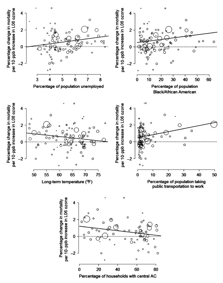
Communities' maximum likelihood estimates and community-specific characteristics for unemployment, race, long-term temperature, public transportation, and central air conditioning (AC), United States, 1987–2000. The size of each circle corresponds to the inverse of the standard error of the community's maximum likelihood estimate; that is, larger circles represent more certain estimates. The bold line reflects results from the univariate second-stage analysis in which the Bayesian hierarchical model was used. Long-term temperature (°C = (°F − 32) × 5/9) included only those days for which ozone data were available. L06, ozone during the previous week (lag 0 days, lag 1 day, lag 2 days … 6 days previous).
Community-specific variables
Summary values of the community-specific descriptor variables are provided in table 1. Several variables were highly correlated, as anticipated. The percentage of the population with a high school education had a correlation of −0.85 and −0.75 with the percentage unemployed and the percentage in poverty, respectively. The percentage in poverty and the percentage unemployed were also related (correlation = 0.83). The percentage of the population with a high school education had a 0.64 correlation with the percentage with a bachelor's degree. Urban and rural variables were near inverses (correlation = −1.0). The percentage of the population driving alone to work and the percentage taking public transportation to work were also related (correlation = −0.97). The correlations between the American Housing Survey national and metropolitan surveys for the 41 communities included in both were 0.97 for central air conditioning and 0.94 for any air conditioning; therefore, we performed analysis by using the national data.
Table 3 shows results from univariate second-stage analysis for each community-specific variable using the Bayesian hierarchical model, and table 4 provides results from the mixed-effects meta-regression model. These tables give the national relative rate estimates for ozone's association with mortality, adjusted for community-specific variables, and the heterogeneity parameter, τ, from univariate second-stage analysis. As noted in the Materials and Methods section, τ2 is the variance unexplained by the community-specific variable. The tables also show the p value for the community-level variable and ρ, the percentage of total variance due to between-study variance (37).
Table 3. Results of the univariate Bayesian hierarchical regression model used to study the short-term effects of ozone exposure on mortality, United States, 1987–2000.
| Community-specific descriptor variable* | Percentage increase in mortality per 10-ppb increase in the previous week's ozone, adjusted for the community-specific variable | Percentage change in effect estimate per IQR† increase in community-level variable | Heterogeneity parameter (τ) | Percentage of total variance due to between-study variance (ρ) | |||
|---|---|---|---|---|---|---|---|
| Central estimate | 95% PI† | Central estimate | 95%PI | p value for community-level variable | |||
| No community-level variables (original analysis) | 0.52 | 0.28, 0.77 | n/a† | n/a | n/a | 0.62 | 20.7 |
| Education | |||||||
| High school degree | 0.49 | 0.24, 0.73 | −48.5 | −110.3, 13.4 | 0.13 | 0.60 | 19.5 |
| Bachelor's degree | 0.52 | 0.28, 0.77 | 6.63 | −55.3, 68.5 | 0.83 | 0.64 | 21.0 |
| Income | |||||||
| Unemployment | 0.49 | 0.26, 0.73 | 68.3 | 3.02, 133.7 | 0.04 | 0.56 | 18.7 |
| Poverty | 0.51 | 0.27, 0.75 | 35.4 | −24.7, 95.4 | 0.25 | 0.60 | 20.0 |
| Median income | 0.52 | 0.28, 0.77 | 9.34 | −42.5, 61.2 | 0.72 | 0.64 | 21.2 |
| Race (Black/African American) | 0.52 | 0.28, 0.75 | 62.2 | 2.94, 121.4 | 0.04 | 0.56 | 18.5 |
| Urbanization | |||||||
| Urban | 0.53 | 0.28, 0.78 | −11.9 | −61.9, 38.1 | 0.64 | 0.64 | 20.7 |
| Rural | 0.53 | 0.28, 0.78 | 12.0 | −38.1, 62.1 | 0.64 | 0.64 | 20.4 |
| Transportation | |||||||
| Drive alone | 0.47 | 0.25, 0.69 | −25.1 | −39.0, −11.3 | <0.01 | 0.44 | 13.5 |
| Use public transportation | 0.47 | 0.25, 0.69 | 20.6 | 9.84, 31.4 | <0.01 | 0.41 | 12.3 |
| Population | 0.46 | 0.22, 0.71 | 9.97 | −2.36, 22.3 | 0.11 | 0.59 | 18.5 |
| Air conditioning | |||||||
| Any air conditioning (n = 76) | 0.56 | 0.28, 0.84 | −32.2 | −112.0, 47.7 | 0.43 | 0.70 | 23.9 |
| Central air conditioning (n = 76) | 0.56 | 0.29, 0.84 | −101.6 | −186.8, −16.3 | 0.02 | 0.64 | 22.2 |
| Weather and pollution | |||||||
| Ozone levels | 0.50 | 0.26, 0.74 | −48.1 | −108.8, 12.7 | 0.12 | 0.61 | 19.3 |
| Ozone levels, April–October | 0.52 | 0.28, 0.76 | −34.0 | −90.1, 22.2 | 0.23 | 0.62 | 20.5 |
| No. of ozone monitors | 0.52 | 0.27, 0.78 | −2.25 | −40.9, 36.4 | 0.91 | 0.65 | 20.4 |
| PM10† levels (n = 93) | 0.52 | 0.27, 0.77 | 15.8 | −45.3, 76.9 | 0.61 | 0.65 | 22.0 |
| PM2.5† levels (n = 90) | 0.53 | 0.28, 0.78 | 46.3 | −25.9, 118.6 | 0.21 | 0.63 | 21.6 |
| Temperature | 0.53 | 0.30, 0.77 | −63.4 | −123.5, −3.25 | 0.04 | 0.57 | 18.8 |
| Dew point temperature | 0.54 | 0.30, 0.77 | −41.3 | −103.4, 20.9 | 0.19 | 0.59 | 19.5 |
n values in parentheses refer to the number of communities used in that analysis.
IQR, interquartile range; PI, posterior interval; n/a, not applicable; PM10, particulate matter with an aerodynamic diameter of ≤10 μm; PM2.5, particulate matter with an aerodynamic diameter of ≤2.5 μm.
Table 4. Results of the mixed-effects meta-regression model used to study the short-term effects of ozone exposure on mortality, United States, 1987–2000.
| Community-specific descriptor variable* | Percentage increase in mortality per 10-ppb increase in the previous week's ozone, adjusted for the community-specific variable | Percentage change in effect estimate per IQR† increase in community-level variable | Heterogeneity parameter (τ) | Percentage of total variance due to between-study variance (ρ) | |||
|---|---|---|---|---|---|---|---|
| Central estimate | 95% PI† | Central estimate | 95% PI | p value for community-level variable | |||
| No community-level variables (original analysis) | 0.52 | 0.29, 0.76 | n/a† | n/a | n/a | 0.58 | 28.3 |
| Education | |||||||
| High school degree | 0.49 | 0.24, 0.73 | −51.1 | −115.0, 12.8 | 0.12 | 0.55 | 18.8 |
| Bachelor's degree | 0.52 | 0.29, 0.76 | 6.56 | −57.6, 70.7 | 0.84 | 0.59 | 22.3 |
| Income | |||||||
| Unemployment | 0.49 | 0.26, 0.72 | 72.0 | 6.70, 137.2 | 0.03 | 0.51 | 16.2 |
| Poverty | 0.51 | 0.27, 0.74 | 37.3 | −24.5, 99.2 | 0.23 | 0.56 | 20.5 |
| Median income | 0.52 | 0.28, 0.76 | 9.56 | −44.1, 63.2 | 0.72 | 0.59 | 22.5 |
| Race (Black/African American) | 0.52 | 0.29, 0.74 | 65.0 | 5.80, 124.2 | 0.03 | 0.51 | 16.1 |
| Urbanization | |||||||
| Urban | 0.53 | 0.29, 0.78 | −12.1 | −63.8, 39.6 | 0.64 | 0.59 | 20.2 |
| Rural | 0.53 | 0.29, 0.78 | 12.1 | −39.6, 63.8 | 0.64 | 0.59 | 21.6 |
| Transportation | |||||||
| Drive alone | 0.47 | 0.26, 0.68 | −26.5 | −39.9, −13.1 | <0.01 | 0.34 | 9.8 |
| Use public transportation | 0.47 | 0.26, 0.68 | 21.5 | 11.4, 31.7 | <0.01 | 0.30 | 7.5 |
| Population | 0.46 | 0.22, 0.71 | 10.4 | −1.8, 22.7 | 0.10 | 0.54 | 17.0 |
| Air conditioning | |||||||
| Any air conditioning (n = 76) | 0.56 | 0.28, 0.83 | −43.1 | −149.3, 63.1 | 0.42 | 0.64 | 26.5 |
| Central air conditioning (n = 76) | 0.57 | 0.30, 0.83 | −102.8 | −186.8, −18.8 | 0.02 | 0.58 | 16.3 |
| Weather and pollution | |||||||
| Ozone levels | 0.50 | 0.26, 0.73 | −50.5 | −112.9, 11.7 | 0.11 | 0.54 | 19.3 |
| Ozone levels, April–October | 0.52 | 0.28, 0.76 | −35.4 | −93.2, 22.5 | 0.23 | 0.56 | 21.5 |
| No. of ozone monitors | 0.53 | 0.28, 0.77 | −1.90 | −40.6, 36.8 | 0.92 | 0.58 | 19.5 |
| PM10† levels (n = 93) | 0.52 | 0.27, 0.76 | 16.8 | −46.2, 79.9 | 0.60 | 0.60 | 23.0 |
| PM2.5† levels (n = 90) | 0.53 | 0.28, 0.78 | 48.3 | −26.3, 122.9 | 0.20 | 0.59 | 22.5 |
| Temperature | 0.53 | 0.31, 0.77 | −66.0 | −127.9, −6.2 | 0.03 | 0.50 | 16.4 |
| Dew point temperature | 0.54 | 0.31, 0.77 | −44.4 | −107.1, 18.3 | 0.16 | 0.53 | 20.2 |
n values in parentheses refer to the number of communities used in that analysis.
IQR, interquartile range; PI, posterior interval; n/a, not applicable; PM10, particulate matter with an aerodynamic diameter of ≤10 μm; PM2.5, particulate matter with an aerodynamic diameter of ≤2.5 μm.
Under both approaches, the ozone and mortality effect estimates were higher for communities in which a higher percentage of the population was unemployed or Black/African American. Higher effect estimates were associated with communities with a higher fraction of the population taking public transportation to work or a lower fraction of persons driving to work. Lower temperatures or prevalence of central air conditioning was associated with higher effect estimates. No relation was observed between PM10 or PM2.5 levels or the number of ozone monitors and the effect estimates for ozone and mortality.
The national relative rate did not vary greatly after adjustment by community-specific variables. When either the Bayesian hierarchical model or the mixed-effects meta-regression results were used, the national relative rate ranged from a 0.46 percent to a 0.54 percent increase in mortality per 10-ppb increase in the previous week's ozone, using variables for which data from all 98 communities were available. Significant heterogeneity remained among the community-specific estimates after adjustment for each community-specific variable, which implies that none of these factors alone explains the variability among communities' relative rates. Of the community-specific variables considered, heterogeneity was most reduced by the percentage of the population that took public transportation to work (ρ was reduced from 20.7 percent to 12.3 percent for the Bayesian hierarchical model).
Figure 1 shows the relation between the community-specific maximum likelihood estimates for ozone and mortality and community values for unemployment, race, public transportation, long-term temperature, and central air conditioning based on the American Housing Survey national survey when the Bayesian hierarchical model was used.
Community-specific variables exhibiting statistically significant associations with ozone and mortality relative rates in univariate second-stage analysis were used in multivariate second-stage regression for both the Bayesian hierarchical regression and the mixed-effects regression models (table 5). For the bivariate analysis, the relation between public transportation and ozone mortality effect estimates was robust to adjustment by race, unemployment, long-term temperature, or central air conditioning. Models including public transportation use showed the largest reduction in heterogeneity (refer to the ρ values in table 5). The associations between higher ozone mortality effect estimates and race, unemployment, long-term temperature, or central air conditioning were not robust to adjustment by public transportation use. We also performed a multivariate analysis by simultaneously including the community-specific variables demonstrating an association with ozone mortality risk estimates in univariate models (table 5). Only the 76 communities with data for all variables were included. The correlation for central air conditioning and long-term temperature was 0.54. None of the individual community-specific variables had a statistically significant relation with ozone mortality effect estimates when all covariates were included together.
Table 5. Results of multivariate Bayesian hierarchical regression and mixed-effects meta-regression models used to study the short-term effects of ozone exposure on mortality, United States, 1987–2000*.
| Bayesian hierarchical regression | Mixed-effects meta-regression | |||||||||
|---|---|---|---|---|---|---|---|---|---|---|
| Percentage change in effect estimates per IQR† increase in community-level variable | τ† | ρ† | Percentage change in effect estimates per IQR increase in community-level variable | τ | ρ | |||||
| Central estimate | 95% PI† | p value | Central estimate | 95% PI | p value | |||||
| Race (Black/African American) | ||||||||||
| Univariate | 62.2 | 2.94, 121.4 | 0.04 | 0.56 | 18.5 | 65.0 | 5.80, 124.2 | 0.03 | 0.51 | 16.1 |
| Adjusted for unemployment | 40.5 | −28.9, 109.8 | 0.25 | 0.55 | 17.8 | 42.3 | −27.6, 112.3 | 0.24 | 0.49 | 15.5 |
| Adjusted for public transportation | 32.0 | −27.1, 91.2 | 0.29 | 0.40 | 12.1 | 34.7 | −24.6, 94.0 | 0.25 | 0.27 | 6.2 |
| Adjusted for long-term temperature | 66.6 | 9.56, 123.7 | 0.02 | 0.49 | 15.5 | 69.8 | 12.9, 126.7 | 0.02 | 0.42 | 13.0 |
| Adjusted for central air conditioning (n = 76) | 73.2 | 10.2, 136.1 | 0.02 | 0.57 | 19.5 | 76.1 | 13.2, 139.0 | 0.02 | 0.50 | 13.6 |
| Adjusted for unemployment, public transportation, long-term temperature, and central air conditioning (n = 76) | 43.8 | −34.7, 122.4 | 0.27 | 0.56 | 18.8 | 45.2 | −34.5, 124.9 | 0.27 | 0.47 | 14.0 |
| Unemployment | ||||||||||
| Univariate | 68.3 | 3.02, 133.7 | 0.04 | 0.59 | 18.7 | 72.0 | 6.70, 137.2 | 0.03 | 0.51 | 16.2 |
| Adjusted for race | 44.8 | −31.6, 121.2 | 0.25 | 0.55 | 17.8 | 47.3 | −29.7, 124.3 | 0.23 | 0.49 | 15.5 |
| Adjusted for public transportation | 25.5 | −42.1, 93.0 | 0.46 | 0.41 | 12.2 | 26.5 | −41.6, 94.5 | 0.45 | 0.31 | 8.0 |
| Adjusted for long-term temperature | 63.6 | 0.10, 121.1 | 0.05 | 0.51 | 16.3 | 66.8 | 3.2, 130.5 | 0.04 | 0.45 | 13.8 |
| Adjusted for central air conditioning (n = 76) | 71.4 | −1.46, 144.2 | 0.05 | 0.60 | 19.8 | 74.2 | 0.7, 147.6 | 0.05 | 0.54 | 14.2 |
| Adjusted for race, public transportation, long-term temperature, and central air conditioning (n = 76) | 24.6 | −65.5, 114.7 | 0.59 | 0.56 | 18.8 | 24.7 | −66.3, 115.8 | 0.60 | 0.47 | 14.0 |
| Public transportation | ||||||||||
| Univariate | 20.6 | 9.84, 31.4 | <0.01 | 0.41 | 12.3 | 21.5 | 11.4, 31.7 | <0.01 | 0.30 | 7.5 |
| Adjusted for race | 18.2 | 6.54, 29.9 | <0.01 | 0.40 | 12.0 | 19.1 | 8.3, 29.8 | <0.01 | 0.27 | 6.2 |
| Adjusted for unemployment | 18.5 | 6.22, 30.8 | <0.01 | 0.41 | 12.2 | 19.3 | 7.6, 31.1 | <0.01 | 0.31 | 8.0 |
| Adjusted for long-term temperature | 18.2 | 6.29, 30.2 | <0.01 | 0.42 | 12.5 | 19.0 | 7.7, 30.4 | <0.01 | 0.30 | 7.5 |
| Adjusted for central air conditioning (n = 76) | 16.2 | 1.97, 30.4 | 0.03 | 0.52 | 16.8 | 17.0 | 2.80, 31.1 | 0.02 | 0.44 | 10.6 |
| Adjusted for race, unemployment, long-term temperature, and central air conditioning (n = 76) | 8.0 | −10.3, 26.3 | 0.39 | 0.56 | 18.8 | 8.7 | −9.0, 26.4 | 0.34 | 0.47 | 14.0 |
| Long-term temperature | ||||||||||
| Univariate | −63.4 | −123.5, −3.25 | 0.04 | 0.57 | 18.8 | −66.0 | −125.9, −6.2 | 0.03 | 0.50 | 16.4 |
| Adjusted for race | −67.3 | −124.7, −9.85 | 0.02 | 0.49 | 15.5 | −70.1 | −126.9, −13.3 | 0.02 | 0.42 | 13.0 |
| Adjusted for unemployment | −58.6 | −117.1, −0.03 | 0.05 | 0.51 | 16.3 | −61.1 | −119.2, −3.0 | 0.04 | 0.45 | 13.8 |
| Adjusted for public transportation | −28.9 | −89.0, 31.3 | 0.35 | 0.42 | 12.5 | −29.9 | −89.3, 29.6 | 0.33 | 0.30 | 7.5 |
| Adjusted for central air conditioning (n = 76) | −27.4 | −114.6, 59.9 | 0.54 | 0.63 | 21.8 | −29.4 | −115.8, 56.9 | 0.51 | 0.57 | 16.0 |
| Adjusted for race, unemployment, public transportation, and central air conditioning (n = 76) | −17.0 | −102.3, 68.4 | 0.70 | 0.56 | 18.8 | −18.7 | −104.9, 66.5 | 0.67 | 0.47 | 14.0 |
| Central air conditioning (n = 76) | ||||||||||
| Univariate | −101.6 | −186.8, −16.3 | 0.02 | 0.64 | 22.2 | −102.8 | −186.8, −18.8 | 0.02 | 0.58 | 16.3 |
| Adjusted for race | −109.5 | −191.9, −27.0 | 0.01 | 0.57 | 19.5 | −110.2 | −190.5, −29.9 | <0.01 | 0.50 | 13.6 |
| Adjusted for unemployment | −96.4 | −180.4, −12.3 | 0.02 | 0.60 | 19.8 | −97.0 | −179.3, −14.7 | 0.02 | 0.54 | 14.2 |
| Adjusted for public transportation | −49.5 | −141.9, 42.4 | 0.29 | 0.52 | 16.8 | −48.9 | −139.4, 41.6 | 0.29 | 0.44 | 10.6 |
| Adjusted for long-term temperature | −81.5 | −187.9, 24.9 | 0.13 | 0.63 | 21.8 | −81.5 | −185.8, 22.8 | 0.13 | 0.57 | 16.0 |
| Adjusted for race, unemployment, public transportation, and long-term temperature (n = 76) | −66.6 | −180.4, 47.3 | 0.25 | 0.56 | 18.8 | −64.1 | −172.9, 44.7 | 0.25 | 0.47 | 14.0 |
n values in parentheses refer to the number of communities used in that analysis.
IQR, interquartile range; τ, heterogeneity parameter; ρ, percentage of total variance due to between-study variance; PI, posterior interval.
We further examined the percentage of the population taking public transportation to work by subway, bus, or railway system to evaluate whether ozone mortality effect estimates were associated with a particular type of public transportation use (table 6). Note that the categories of subway, bus, or rail are subsets of the public transportation category. On average across the communities, bus use accounted for the majority of public transportation used. The variables of subway, bus, and rail use exhibited associations with each other (correlations ranged from 0.44 to 0.52). All three types of public transportation use were associated with higher effect estimates for ozone and mortality. New York City, New York, had the highest public transportation use at 50 percent. The relation between higher public transportation use and higher ozone mortality effect estimates was robust to exclusion of New York City.
Table 6. Percentage change in ozone mortality effect estimate for an IQR* increase in the percentage of the adult population using various types of public transportation to travel to work, Bayesian hierarchical model, United States, 1987–2000.
| Mean | IQR | Percentage change per IQR | ||
|---|---|---|---|---|
| Central estimate | 95% PI* | |||
| Any public transportation | 5.48 | 3.05 | 20.6 | 9.84, 31.4 |
| Subway | 1.17 | 0.03 | 0.25 | 0.08, 0.41 |
| Bus | 3.85 | 3.02 | 44.0 | 15.1, 73.0 |
| Rail | 0.20 | 0.12 | 16.5 | 7.52, 25.4 |
IQR, interquartile range; PI, posterior interval.
Discussion
Socioeconomic inequalities and race have been linked to a higher burden of environmental risks, including those from air pollution (38–51). For example, lower PM10 effect estimates for mortality were observed for communities with higher income and educational levels (47). Regional and seasonal differences in the association of particulate matter with mortality and hospital admissions (15, 34–36, 52) may be the result of dissimilar chemical composition; however, differences in exposure and community-level characteristics may also play a role. The elevated impact of air pollution on Black/African-American and high-unemployment neighborhoods may relate to differential residential exposure, access to health care, baseline health status, occupational exposure, underlying health status, or other factors (38, 39).
The associations of racial and socioeconomic characteristics with ozone's effects on health have been researched in a limited number of studies. Time-series analysis of respiratory hospital admissions in New York City found higher effect estimates for non-Whites compared with Whites (53), mirroring results from this study. Socioeconomic status did not modify the relation between ozone and hospital admissions for the elderly or children in Vancouver, Canada (54). A study of mortality in Mexico City, Mexico, did not identify consistent patterns by socioeconomic gradients at county-level resolution; however, it noted that the study may not have been able to fully illuminate such associations (46). Socioeconomic level as measured by father's educational status affected pulmonary response to ozone in a study of 372 persons aged 18–35 years (48). A human exposure study for the South Coast Air Basin of California found that low-income areas may on average experience higher ozone concentrations than higher-income areas (55). However, for the 98 US communities in this study, we observed similar ozone levels for communities below and above the median percentage in poverty (26.91 ppb and 26.71 ppb, respectively).
Two multicity US studies found that effect estimates for hospital admissions decreased for PM10 (56) and ozone with an increasing percentage of homes with central air conditioning (57). We also observed this result with an interquartile-range increase in households with central air conditioning associated with a 101.6 percent decrease in effect estimates for ozone's impact on mortality. The relative impacts of central air conditioning and long-term temperature were difficult to disentangle in this study because of their relation (correlation coefficient = 0.54). High correlation among community characteristics also limited more detailed multivariate analysis with additional variables.
Results indicated no association between ozone effect estimates for mortality and long-term PM10 or PM2.5 levels. This finding provides further evidence that the relation between ozone and mortality is not confounded by particulate pollution, as shown in several meta-analyses (7, 9, 11, 58) and multicity studies (1, 3, 4). Earlier time-series analysis found national and community-specific ozone and mortality effect estimates to be robust to inclusion of PM10 levels (1). No statistically significant association was observed between effect estimates and long-term ozone levels under the Bayesian hierarchical or the mixed-effects meta-regression approach. These results could indicate the absence of a threshold level, as was demonstrated in earlier research (5). If a threshold exists, lower relative rates could be observed for communities with lower ozone levels.
Higher effect estimates for communities with higher use of public transportation may be the result of differential exposure patterns for ozone or an indication of a relation between mortality and a pollutant associated with public transportation whose patterns are similar to those for ozone. Further research is needed to investigate this relation. Note that this link does not imply that public transportation use results in more ozone-related deaths because higher public transportation use was also associated with lower long-term ozone levels. For every 10 percent of the population that takes public transportation to work, long-term ozone levels decreased 9 percent when evaluation was conducted at the mean ozone level (p < 0.001).
Although this study found an indication of a gradient for the effect of ozone on mortality by socioeconomic status, there are important limitations. Our analysis assumed that the between-community associations of descriptor variables do not vary with time; however, income levels and other indicators of socioeconomic status can change for communities and for individuals, thereby diluting our socioeconomic indicators. Heterogeneity among socioeconomic factors is likely to exist at the community level and can be present in smaller aggregated units such as census block groups (59). Even with individual data, the choice of socioeconomic indicator is complex given that true socioeconomic position is a function of multiple factors including income, occupation, deprivation, social class, and education, among others; and no single factor completely accounts for the relation between socioeconomic status and health (59). For example, median household income does not address capital assets, number of adults and children in the household, source of the income (e.g., wage earnings vs. child support), long-term income history, and true purchasing power of a given monetary amount, which can vary by community.
We used community-level descriptors rather than individual-level data, which could generate misclassification bias (60–62). Even though we explored effect modification by particles, we did not consider the chemical composition of the particulate mixture. Ambient measurements were applied as a surrogate of personal exposure, and, in fact, many of the results may relate to differences in exposure patterns (e.g., different exposures by unemployment status) rather than or in addition to differences in baseline health status. Furthermore, we did not consider other potential differences among populations that reflect underlying health status, such as smoking patterns.
In summary, this research examined whether short-term effects of ozone on mortality are modified by community-specific characteristics by using data for 14 years for more than 40 percent of the US population to estimate effect modification, accounting for within-community and between-community variance. We explored the sensitivity of results with two modeling software approaches to estimating effect modification: 1) Bayesian hierarchical modeling (28) and 2) mixed-effects meta-regression modeling (30–32).
Our results indicate stronger effects in some regions than others, but the 95 percent posterior intervals for results from all regions overlapped (table 2). We found that heterogeneity among community-specific effect estimates can be partially explained by community-level indicators. Specifically, our findings indicate that some populations (i.e., Black/African American and the unemployed) may bear a higher health burden from ozone and that a higher prevalence of central air conditioning may modify ozone exposure, thereby lessening its health impacts.
Supplementary Material
Acknowledgments
The US Environmental Protection Agency (purchase no. EP05C000125), the Johns Hopkins CDC Center of Excellence for Environmental Public Health Tracking (U50/CCU322417), the National Institute for Environmental Health Sciences (ES012054-01, P30 ES 03819), and the Health Effects Institute Walter A. Rosenblith New Investigator Award (4720-RFA04-2/04-16) funded this research.
The authors thank Keita Ebisu of Yale University and Aidan McDermott and Suyan Tian of the Johns Hopkins Bloomberg School of Public Health.
The views expressed in this article are those of the authors and do not necessarily reflect the views or policies of the funding agencies.
Abbreviations
- PM2.5
particulate matter with an aerodynamic diameter of ≤2.5 μm
- PM10
particulate matter with an aerodynamic diameter of ≤10 μm
Footnotes
Conflict of interest: none declared.
References
- 1.Bell ML, McDermott A, Zeger SL, et al. Ozone and short-term mortality in 95 US urban communities, 1987–2000. JAMA. 2004;292:2372–8. doi: 10.1001/jama.292.19.2372. [DOI] [PMC free article] [PubMed] [Google Scholar]
- 2.Huang Y, Dominici F, Bell ML. Bayesian hierarchical distributed lag models for summer ozone exposure and cardiorespiratory mortality. Environmetrics. 2005;16:547–62. doi: 10.1002/env.721. [DOI] [PMC free article] [PubMed] [Google Scholar]
- 3.Gryparis A, Forsberg B, Katsouyanni K, et al. Acute effects of ozone on mortality from the “air pollution and health: a European approach” project. Am J Respir Crit Care Med. 2004;170:1080–7. doi: 10.1164/rccm.200403-333OC. [DOI] [PubMed] [Google Scholar]
- 4.Schwartz J. How sensitive is the association between ozone and daily deaths to control for temperature? Am J Respir Crit Care Med. 2005;171:627–31. doi: 10.1164/rccm.200407-933OC. [DOI] [PubMed] [Google Scholar]
- 5.Bell ML, Peng RD, Dominici F. The exposure-response curve for ozone and risk of mortality and the adequacy of current ozone regulations. Environ Health Perspect. 2006;114:532–6. doi: 10.1289/ehp.8816. [DOI] [PMC free article] [PubMed] [Google Scholar]
- 6.Filleul L, Cassadou S, Médina S, et al. The relation between temperature, ozone, and mortality in nine French cities during the heat wave of 2003. Environ Health Perspect. 2006;114:1344–7. doi: 10.1289/ehp.8328. [DOI] [PMC free article] [PubMed] [Google Scholar]
- 7.Bell ML, Dominici F, Samet JM. A meta-analysis of time-series studies of ozone and mortality with comparison to the National Morbidity, Mortality and Air Pollution Study. Epidemiology. 2005;16:436–45. doi: 10.1097/01.ede.0000165817.40152.85. [DOI] [PMC free article] [PubMed] [Google Scholar]
- 8.Anderson HR, Atkinson RW, Peacock JL, et al. Report of a WHO Task Group. Copenhagen, Denmark: World Health Organization; 2004. Meta-analysis of time-series studies and panel studies of particulate matter (PM) and ozone (O3) [Google Scholar]
- 9.Ito K, De Leon SF, Lippmann M. Associations between ozone and daily mortality: analysis and meta-analysis. Epidemiology. 2005;16:446–57. doi: 10.1097/01.ede.0000165821.90114.7f. [DOI] [PubMed] [Google Scholar]
- 10.Levy JI, Chemerynski SM, Sarnat JA. Ozone exposure and mortality: an empiric Bayes metaregression analysis. Epidemiology. 2005;16:458–68. doi: 10.1097/01.ede.0000165820.08301.b3. [DOI] [PubMed] [Google Scholar]
- 11.Thurston GD, Ito K. Epidemiological studies of acute ozone exposures and mortality. J Expo Anal Environ Epidemiol. 2001;11:286–94. doi: 10.1038/sj.jea.7500169. [DOI] [PubMed] [Google Scholar]
- 12.Levy JI, Carrothers TJ, Tuomisto JT, et al. Assessing the public health benefits of reduced ozone concentrations. Environ Health Perspect. 2001;109:1215–26. doi: 10.1289/ehp.011091215. [DOI] [PMC free article] [PubMed] [Google Scholar]
- 13.Blondeau P, Iordache V, Poupard O, et al. Relationship between outdoor and indoor air quality in eight French schools. Indoor Air. 2005;15:2–12. doi: 10.1111/j.1600-0668.2004.00263.x. [DOI] [PubMed] [Google Scholar]
- 14.Weschler CJ. Ozone in indoor environments: concentration and chemistry. Indoor Air. 2000;10:269–88. doi: 10.1034/j.1600-0668.2000.010004269.x. [DOI] [PubMed] [Google Scholar]
- 15.Peng RD, Dominici F, Pastor-Barriuso R, et al. Seasonal analysis of air pollution and mortality in 100 US cities. Am J Epidemiol. 2005;161:585–94. doi: 10.1093/aje/kwi075. [DOI] [PubMed] [Google Scholar]
- 16.US Census Bureau. Census 2000. Summary File 1. Washington, DC: US Census Bureau; 2000. [Google Scholar]
- 17.US Census Bureau. Census 2000. Summary File 3. Washington, DC: US Census Bureau; 2000. [Google Scholar]
- 18.US Census Bureau. Census 1990. Summary File 3. Washington, DC: US Census Bureau; 1990. [Google Scholar]
- 19.US Census Bureau. Census 1990. Summary File 1. Washington, DC: US Census Bureau; 1990. [Google Scholar]
- 20.US Department of Commerce, US Department of Housing and Urban Development. American Housing Survey. Washington, DC: US Department of Commerce, US Department of Housing and Urban Development; 1998. [Google Scholar]
- 21.US Department of Commerce, US Department of Housing and Urban Development. American Housing Survey. Washington, DC: US Department of Commerce, US Department of Housing and Urban Development; 1994. [Google Scholar]
- 22.US Department of Commerce, US Department of Housing and Urban Development. American Housing Survey. Washington, DC: US Department of Commerce, US Department of Housing and Urban Development; 1999. [Google Scholar]
- 23.US Department of Commerce, US Department of Housing and Urban Development. American Housing Survey. Washington, DC: US Department of Commerce, US Department of Housing and Urban Development; 1993. [Google Scholar]
- 24.US Department of Commerce, US Department of Housing and Urban Development. American Housing Survey. Washington, DC: US Department of Commerce, US Department of Housing and Urban Development; 1989. [Google Scholar]
- 25.US Department of Commerce, US Department of Housing and Urban Development. American Housing Survey. Washington, DC: US Department of Commerce, US Department of Housing and Urban Development; 1991. [Google Scholar]
- 26.US Department of Commerce, US Department of Housing and Urban Development. American Housing Survey. Washington, DC: US Department of Commerce, US Department of Housing and Urban Development; 1997. [Google Scholar]
- 27.Welty LJ, Zeger SL. Are the acute effects of particulate matter on mortality in the National Morbidity, Mortality, and Air Pollution Study the result of inadequate control for weather and season? A sensitivity analysis using flexible distributed lag models. Am J Epidemiol. 2005;162:80–8. doi: 10.1093/aje/kwi157. [DOI] [PubMed] [Google Scholar]
- 28.Dominici F. Invited commentary: air pollution and health—what can we learn from a hierarchical approach? Am J Epidemiol. 2002;155:11–15. doi: 10.1093/aje/155.1.11. [DOI] [PubMed] [Google Scholar]
- 29.Everson PJ, Morris CN. Inference for multivariate normal hierarchical models. J R Stat Soc (B) 2000;62:399–412. [Google Scholar]
- 30.Stram DO. Meta-analysis of published data using a linear mixed-effects model. Biometrics. 1996;52:536–44. [PubMed] [Google Scholar]
- 31.Smith-Warner SA, Spiegelman D, Ritz J, et al. Methods for pooling results of epidemiologic studies: the pooling project of prospective studies of diet and cancer. Am J Epidemiol. 2006;163:1053–64. doi: 10.1093/aje/kwj127. [DOI] [PubMed] [Google Scholar]
- 32.DerSimonian R, Laird N. Meta-analysis in clinical trials. Control Clin Trials. 1986;7:177–88. doi: 10.1016/0197-2456(86)90046-2. [DOI] [PubMed] [Google Scholar]
- 33.Harbord R, Steichen T. Metareg: Stata module to perform meta-analysis regression. Boston, MA: Boston College Department of Economics; 2005. [Google Scholar]
- 34.Samet JM, Zeger SL, Dominici F, et al. The National Morbidity, Mortality, and Air Pollution Study Part II: morbidity and mortality from air pollution in the United States. Cambridge, MA: Health Effects Institute; 2000. [PubMed] [Google Scholar]
- 35.Samet JM, Dominici F, Zeger SL, et al. The National Morbidity, Mortality, and Air Pollution Study Part I: methods and methodologic issues. Cambridge, MA: Health Effects Institute; 2000. [PubMed] [Google Scholar]
- 36.Dominici F, McDermott A, Zeger SL, et al. National maps of the effects of particulate matter on mortality: exploring geographical variation. Environ Health Perspect. 2003;111:39–43. doi: 10.1289/ehp.5181. [DOI] [PMC free article] [PubMed] [Google Scholar]
- 37.Takkouche B, Cadarso-Suárez C, Spiegelman D. Evaluation of old and new tests of heterogeneity in epidemiologic meta-analysis. Am J Epidemiol. 1999;150:206–15. doi: 10.1093/oxfordjournals.aje.a009981. [DOI] [PubMed] [Google Scholar]
- 38.Bell ML, O'Neill MS, Cifuentes LA, et al. Challenges and recommendations for the study of socioeconomic factors and air pollution health effects. Environ Sci Policy. 2005;8:525–33. [Google Scholar]
- 39.O'Neill MS, Jerrett M, Kawachi K, et al. Health, wealth, and air pollution: advancing theory and methods. Environ Health Perspect. 2003;111:1861–70. doi: 10.1289/ehp.6334. [DOI] [PMC free article] [PubMed] [Google Scholar]
- 40.American Lung Association. Urban air pollution and health inequities: a workshop report. Environ Health Perspect. 2001;109 3:S357–74. [PMC free article] [PubMed] [Google Scholar]
- 41.Evans GW, Kantrowitz E. Socioeconomic status and health: the potential role of environmental risk exposure. Annu Rev Public Health. 2002;23:303–31. doi: 10.1146/annurev.publhealth.23.112001.112349. [DOI] [PubMed] [Google Scholar]
- 42.Apelberg BJ, Buckley TJ, White RH. Socioeconomic and racial disparities in cancer risk from air toxics in Maryland. Environ Health Perspect. 2005;113:693–9. doi: 10.1289/ehp.7609. [DOI] [PMC free article] [PubMed] [Google Scholar]
- 43.Wheeler BW, Ben-Shlomo Y. Environmental equity, air quality, socioeconomic status, and respiratory health: a linkage analysis of routine data from the Health Survey of England. J Epidemiol Community Health. 2005;59:948–54. doi: 10.1136/jech.2005.036418. [DOI] [PMC free article] [PubMed] [Google Scholar]
- 44.Jerrett M, Buzzelli M, Burnett RT, et al. Particulate air pollution, social confounders, and mortality in small areas of an industrial city. Soc Sci Med. 2005;60:2845–63. doi: 10.1016/j.socscimed.2004.11.006. [DOI] [PubMed] [Google Scholar]
- 45.Gouveia N, Fletcher T. Time series analysis of air pollution and mortality: effects by cause, age, and socioeconomic status. J Epidemiol Community Health. 2000;54:750–5. doi: 10.1136/jech.54.10.750. [DOI] [PMC free article] [PubMed] [Google Scholar]
- 46.O'Neill MS, Loomis D, Borja-Aburto VH. Ozone, area social conditions, and mortality in Mexico City. Environ Res. 2004;94:234–42. doi: 10.1016/j.envres.2003.07.002. [DOI] [PubMed] [Google Scholar]
- 47.Martins MC, Fatigati FL, Véspoli TC, et al. Influence of socio-economic conditions on air pollution adverse health effects in elderly people: an analysis of six regions of São Paulo, Brazil. J Epidemiol Community Health. 2004;58:41–6. doi: 10.1136/jech.58.1.41. [DOI] [PMC free article] [PubMed] [Google Scholar]
- 48.Ito K, Thurston GD. Daily PM10/mortality associations: an investigation of at-risk subpopulations. J Expo Anal Environ Epidemiol. 1996;6:79–95. [PubMed] [Google Scholar]
- 49.Zanobetti A, Schwartz J, Dockery DW. Airborne particles are a risk factor for hospital admissions for heart and lung disease. Environ Health Perspect. 2000;108:1071–7. doi: 10.1289/ehp.001081071. [DOI] [PMC free article] [PubMed] [Google Scholar]
- 50.Cakmak S, Dales RE, Judek S, et al. Does socio-demographic status influence the effect of pollens and molds on hospitalization for asthma? Results from a time-series study of 10 Canadian cities. Ann Epidemiol. 2005;15:214–18. doi: 10.1016/j.annepidem.2004.06.001. [DOI] [PubMed] [Google Scholar]
- 51.Lin M, Chen Y, Villeneuve PJ, et al. Gaseous air pollutants and asthma hospitalization of children with low household income in Vancouver, British Columbia, Canada. Am J Epidemiol. 2004;159:294–303. doi: 10.1093/aje/kwh043. [DOI] [PubMed] [Google Scholar]
- 52.Dominici F, Peng RD, Bell ML, et al. Fine particulate air pollution and hospital admission for cardiovascular and respiratory diseases. JAMA. 2006;295:1127–34. doi: 10.1001/jama.295.10.1127. [DOI] [PMC free article] [PubMed] [Google Scholar]
- 53.Gwynn RC, Thurston GD. The burden of air pollution: impacts among racial minorities. Environ Health Perspect. 2001;109 4:S501–6. doi: 10.1289/ehp.01109s4501. [DOI] [PMC free article] [PubMed] [Google Scholar]
- 54.Yang Q, Chen Y, Shi Y, et al. Association between ozone and respiratory admissions among children and the elderly in Vancouver, Canada. Inhal Toxicol. 2003;15:1297–308. doi: 10.1080/08958370390241768. [DOI] [PubMed] [Google Scholar]
- 55.Korc ME. A socioeconomic assessment of human exposure to ozone in the South Coast Air Basin of California. J Air Waste Manag Assoc. 1996;46:547–57. doi: 10.1080/10473289.1996.10467490. [DOI] [PubMed] [Google Scholar]
- 56.Janssen NAH, Schwartz J, Zanobetti A, et al. Air conditioning and source-specific particles as modifiers of the effect of PM10 on hospital admissions for heart and lung disease. Environ Health Perspect. 2002;110:43–9. doi: 10.1289/ehp.0211043. [DOI] [PMC free article] [PubMed] [Google Scholar]
- 57.Medina-Ramón M, Zanobetti A, Schwartz J. The effect of ozone and PM10 on hospital admissions for pneumonia and chronic obstructive pulmonary disease: a national multicity study. Am J Epidemiol. 2006;163:579–88. doi: 10.1093/aje/kwj078. [DOI] [PubMed] [Google Scholar]
- 58.Stieb DM, Judek S, Burnett RT. Meta-analysis of time-series studies of air pollution and mortality: effects of gases and particles and the influence of cause of death, age, and season. J Air Waste Manage Assoc. 2002;52:470–84. doi: 10.1080/10473289.2002.10470794. [DOI] [PubMed] [Google Scholar]
- 59.Krieger N, Williams DR, Moss NE. Measuring social class in US public health research: concepts, methodologies, and guidelines. Annu Rev Public Health. 1997;18:341–78. doi: 10.1146/annurev.publhealth.18.1.341. [DOI] [PubMed] [Google Scholar]
- 60.Zeger SL, Thomas D, Dominici F, et al. Exposure measurement error in time-series studies of air pollution: concepts and consequences. Environ Health Perspect. 2000;108:419–26. doi: 10.1289/ehp.00108419. [DOI] [PMC free article] [PubMed] [Google Scholar]
- 61.Shy C, Kleinbaum D, Morgenstern H. The effect of misclassification of exposure status in epidemiological studies of air pollution health effects. J Urban Health. 1978;54:1155–65. [PMC free article] [PubMed] [Google Scholar]
- 62.Sheppard L, Slaughter JC, Schildcrout J, et al. Exposure and measurement contributions to estimates of acute air pollution effects. J Expo Anal Environ Epidemiol. 2005;15:366–76. doi: 10.1038/sj.jea.7500413. [DOI] [PubMed] [Google Scholar]
Associated Data
This section collects any data citations, data availability statements, or supplementary materials included in this article.