Statistical models for quantifying diagnostic accuracy with multiple lesions per patient

Abstract

We propose random-effects models to summarize and quantify the accuracy of the diagnosis of multiple lesions on a single image without assuming independence between lesions. The number of false-positive lesions was assumed to be distributed as a Poisson mixture, and the proportion of true-positive lesions was assumed to be distributed as a binomial mixture. We considered univariate and bivariate, both parametric and nonparametric mixture models. We applied our tools to simulated data and data of a study assessing diagnostic accuracy of virtual colonography with computed tomography in 200 patients suspected of having one or more polyps.

1. INTRODUCTION

Diagnostic accuracy is usually summarized with the true-positive rate (TPR) or sensitivity and the false-positive rate (FPR) or one minus specificity. Some diagnostic tasks are more complicated than simple detection of a single occurrence of the (abnormal) condition, and in such cases calculating TPR and FPR may prove difficult. In this paper, we will discuss as an example the diagnostic accuracy of virtual colonography in locating colonic polyps and documenting their size or severity. Accurate sensitive diagnosis is essential as polyps may develop into tumor tissue, but diagnosis must also be sufficiently specific to minimize invasive procedures. Patients often have more than one polyp, any of which may be seen or missed. Other examples of such a diagnostic situation are occurrence of multiple lesions using mammography or multiple infarcts using computed tomography (CT) or magnetic resonance imaging in a patient suspected of having a stroke.

Zhou and others (2002, p. 43) describe several methods of summarizing diagnostic accuracy for such data. Often seen is the so called “per-lesion” approach. Sensitivity is calculated as the fraction of correctly identified polyps. It seems clinically meaningful to assess sensitivity in the case of polyps because of the importance to diagnose each polyp. Specificity is, however, difficult to define in this case because there is an almost infinite number of locations in the colon where there could be a polyp. Zhou and others (2002) suggested a simple way of addressing this difficulty by dividing the image (colon in this case) into segments and calculating sensitivity and specificity per segment. Unfortunately, however, it is not always obvious how to define segments. The approach also weighs equally the segments with one or many true- or false-positive (TP or FP) polyps, whereas, intuitively, a segment with many polyps contains more information than a segment with only one. Egan and Schulman (1961), Bunch and others (1978), and Chakraborty and Winder (1990) developed the “free-response receiver-operator-characteristic (ROC) curve (FROC)” to analyze multiple lesions. The y-axis of the FROC curve is the probability of both detecting and correctly locating the lesions; the x-axis is the average number of FPs per patient. The summary measure of the FROC curve may be interpreted as the average fraction of lesions detected on an image before an observer makes an FP error. Unfortunately, the approach assumes independence between multiple findings on the same image of a patient.

In this paper, we propose random-effects models to summarize and quantify the accuracy of the diagnosis of multiple lesions on a single image without the independence assumption. In Section 2, we describe the statistical model underlying our approach. In section 4, we apply our tool to the data of a study assessing diagnostic accuracy of virtual colonography with CT in 200 patients suspected of having one or more polyps.

2. METHODS

We consider the situation where N patients undergo a diagnostic test to detect and localize possibly multiple lesions. For each patient, a gold standard is required such that for each lesion identified by the diagnostic test, it is known whether it is an FP or a TP diagnosis.

2.1. Specificity

Since the exact locations of the FPs are of lesser importance, we consider the number of FP lesions in patient i,X_i, say, and assume that X_i follows the Poisson distribution with expectation μ. The specificity is then defined as the probability of zero FP lesions in a patient: Pr(X=0|μ)=e^−μ. Given a sample of observations x₁,…,x_N, the maximum likelihood estimator of the parameter μ is = ∑_ix_i/N with standard error se()=, and the 95% confidence interval of the specificity is given by exp(−±1.96×se()) (Johnson and others, 1992).

The assumption of a common FPR across patients is often too restrictive, and often the variance of the number of FPs is larger than the mean, thus violating the Poisson assumption. A common method to relax this independence assumption is to assume that the intensity parameter varies randomly between patients, according to a distribution with density g(μ|θ). Specificity is now defined as

(2.1)

a weighted average of specificity values across patients with weights given by g(μ|θ).

The density function g(·) is unknown and must be estimated from the data. The most commonly used approach is to assume a gamma distribution g(μ|a,b). The integral has a closed-form solution, and the specificity is then

(2.2)

Maximum likelihood estimates of (a,b) are easy to calculate (see, e.g. Johnson and others, 1997) but have no simple equation. It is also awkward to estimate the 95% confidence interval of the specificity, but a nonparametric bootstrap procedure performs well.

Other parametric functions for g(·) can be used (e.g. a log-normal distribution), but in general there is little evidence to justify any particular choice. One might therefore prefer to specify a fully nonparametric distribution for g(·) (Carlin and Louis, 1996, p. 51). Laird (1978) proved that the nonparametric maximum likelihood estimate of g(·) is a discrete distribution with at most N mass points. Assume that g(·) has mass points θ=(θ₁,…,θ_J) with probabilities w=(w₁,…,w_J), where J≤N, then the likelihood of observations x₁,x₂,…,x_N is given by

(2.3)

Iteratively, this likelihood is easily maximized as a function of θ and w using an expectation-maximization (EM) algorithm (Carlin and Louis, 1996). Given maximum likelihood estimates of and , specificity is estimated as Pr(X=0)=. In this case, calculating the 95% confidence interval is very awkward too, but we have found that a nonparametric bootstrap approach works well.

2.2. Sensitivity

In contrast to FPs, the exact locations of the TP lesions are of primary importance, and we therefore consider the outcome of the diagnostic test for each lesion in patient i separately. Define Y_ij as the result of the diagnostic test at the location of the jth lesion in patient i:Y_ij=1 when the diagnostic test is positive and Y_ij=0 if it is negative.

Sensitivity is defined as the probability of a TP test result. As with the specificity, we allow sensitivity γ_i to vary between patients. Given γ_i, the outcomes of the diagnostic testing in patient i at locations j and l,y_ij and y_il, are assumed to be independent for all j,l. The likelihood of the test results of k_i lesions, y_i1,…,y_iki, therefore equals L(y_i|γ_i)=. When k_i is small, the maximum likelihood estimate of γ_i is very unstable. For this reason, we again assume that in the population of patients γ follows a distribution with density g(γ|θ). A common choice for g(·) is the beta distribution with parameters θ=(a,b) (Ryea and others, 2007). The likelihood of the observations y_i given θ=(a,b) is L(y_i|(a,b))=∫₀¹L(y_i|γ)g(γ|(a,b))dγ. Again the beta distribution is a convenient choice because the integral in the likelihood has a closed-form solution.

Again there is usually little evidence to prefer a particular distribution, and therefore one might again prefer a nonparametric specification. As in case of the specificity, we use a discrete distribution with J classes with mass points θ=(θ₁,…,θ_J) and probabilities w=(w₁,…,w_J), where J≤N. The likelihood of the diagnostic testing of the k_i lesions in patient i is given by

(2.4)

This likelihood is also iteratively maximized as a function of θ and w using an EM algorithm.

Given the maximum likelihood estimates and , the (per-lesion) sensitivity is estimated as . Again we use a bootstrap approach to estimate the 95% confidence interval. The probability that there is at least one TP lesion in a patient (the “per-patient sensitivity”) equals , where k is the (mean) number of lesions in the patients.

2.3. A generalization and an alternative

The model can be generalized in several ways. First, both specificity and sensitivity may depend on observed patient characteristics. Including this dependence in the model may explain the variation between patients. For the FP lesions, the logarithm of the Poisson intensity parameter μ_i in patient i may depend on a linear fashion of a set of covariate values observed in i:logμ_i=β₀+β_1zi1+…+e_i, where β is a regression parameter and e_i is a residual component. The lesion-specific sensitivity of patient i may also be modeled as a function of covariates, logit(γ_i)=β₀+β_1zi1+…+e_i.

Instead of modeling the correlations between (false) lesions in the same patient with a random effect, these correlations may be ignored. The analysis then boils down to simple Poisson and binomial regressions, and the associated standard errors can be corrected with a generalized estimation equation approach (Martus and others, 2004).

2.4. Bivariate relation between specificity and sensitivity

Multiple-lesion data allow estimation of the relation between the per-patient specificity and the per-lesion sensitivity, “even with only one cutpoint”. The relation can be directly modeled in a bivariate random-effects model in order to obtain the ROC curve. In such a model, the Poisson parameter υ_i=log(μ_i) and the logit-transformed parameter ξ_i=logit(γ_i) are assumed to have a bivariate distribution g(υ,ξ) across patients, where it helps to model ξ_i as ξ_i=a+bυ_i+ϵ_i. An obvious choice for g(·) is the bivariate normal with expectations =a+b× and covariance matrix 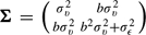. The likelihood of the observations of patient 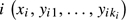is

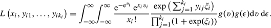(2.5)

This model can be estimated in standard software such as SAS proc NLMIXED, and a Bayesian version is easily implemented in Winbugs.

Instead of the bivariate normal distribution, a nonparametric distribution can be used which is defined by a 2-dimensional grid of points θ_rs with weights w_rs(r=1,…,R;s=1,…,S). The likelihood of patient i is then

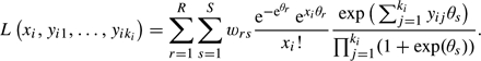(2.6)

This model is not readily available in standard software, but the log-likelihood is easily maximized with an EM algorithm.

3. SIMULATION

We simulated data somewhat according to the example of diagnosing colon polyps (lesions) with virtual colonography, which we will discuss in Section 4. We performed several simulations, and we will show an extreme and slightly pathological example. For ease of the simulation, lesions (and nonlesions) were assumed to be characterized by one variable only, which we might call the lesion thickness, and that each patient consisted of 50 locations. Data for 50 patients at the 50 locations were simulated as follows. First, the number of true lesions per patient was sampled from the Poisson distribution with expectation of 5 lesions. The thickness of each lesion per patient was sampled from a normal distribution; the means and variances of this distribution varied between patients, and these patient-specific parameters were sampled themselves from a normal distribution (mean) and a gamma distribution (variance) with fixed parameters. The thickness variable at the nonlesion locations was also sampled from a normal distribution with means and variances sampled from normal and gamma distributions. Finally, a threshold was chosen such that the overall number of identified true lesions was a fixed number (30%, 50%, or 70%), and afterwards, the number of FP lesions and the number of TP lesions were counted for each patient.

We discuss results from one simulation with a threshold chosen such that 50% of all lesions were identified. In the 50 patients, the number of lesions varied between 0 (in 1 patient) and 9 with a mean of 4.8 and standard deviation 2.0. There were 1124 FP lesions, and the number of FP lesions varied between 0 and 49 per patient with mean 22.48 and variance 388.87, see Figure 1. The histogram seems to consist of 3 subgroups of patients with few, moderate, or large numbers of FP lesions. The gamma and normal distributions for the random effect will probably not fit well for these data, and this example will therefore favor the nonparametric approach.

Fig. 1.

Histogram of the number of FP lesions per patient in the simulated data.

There were 14 patients without FP lesions, and the specificity could therefore be calculated as 14/50=28%. According to the simple Poisson model (log-likelihood ℓ∝−644.97), the intensity μ is estimated as 22.48(se=0.67) and the specificity is therefore e^−22.48≈0%, which is clearly much too low. The generalized estimation equation (GEE) approach, implemented in SAS proc genmod, does not correct this bias but does increase the standard error of the estimate to 2.76. The parameters of the gamma–Poisson model (log-likelihood ℓ∝−198.38) were estimated as log(a)=−0.84 and log(b)=−3.95 yielding an intensity estimate of e^{log(a)−log(b)}=22.42 and specificity 18%, which is still too low. The log-normal–Poisson mixture model had a similar estimate of the specificity (15%). The nonparametric Poisson mixture (log-likelihood ℓ∝−164.63) resulted in a mixture of 4 patient subgroups: patients with an intensity of 0.01 FPs (weight w=0.30), patients with about 7 FPs (w=0.13), patients with about 18 FPs (w=0.11), and patients with about 42 FPs (w=0.46). The estimated specificity is 28% with 95% confidence interval (17−42%). Note that this estimate corresponds with the ratio of number of patients without FPs to the total number of patients. This correspondence was seen in almost all simulations.

A total of 234 lesions were present in 49 out of the 50 simulated patients, and the number varied between 1 and 9 with mean 4.8 (standard deviation 2.0). By choosing our threshold, 117 lesions were identified yielding lesion sensitivity of 117/234=50%. The log-likelihood of this binomial model was ℓ=−130.21. There were 32 patients in whom at least one lesion was identified (32/49=65%). For a patient with 4 lesions, the probability of observing at least one lesion is therefore 1−(1−0.50)⁴=94%. The observed proportion of identified lesions per patient varied between 0 and 1 with mean 0.49 and standard deviation 0.44. This variation cannot be explained by sampling only since the beta-binomial model (ℓ=−74.15) and the logit-normal–binomial model fitted better than the binomial model. The mean lesion sensitivity was 50% in both models, but the probability of observing at least one lesion in a patient with 4 lesions is much smaller: about 65%. The nonparametric binomial mixture model had log-likelihood ℓ=−76.29 and yielded 3 subgroups of patients with lesion sensitivity of 9%, 47%, and 90% and weights 45%, 11%, and 44%, respectively. The probability of observing at least one lesion in a patient with 4 lesions was 65%. Note the close correspondence between the “estimated” probabilities of the random-effect models of identifying at least one lesion in a patient with the “observed” rate of patients with at least one lesion identified. Again this was observed in almost all simulations.

The log-likelihood of the nonparametric bivariate model was −234.17, which was slightly larger than the sum of the 2 likelihoods of the 2 nonparametric mixture models (−164.63)+(−76.29)=−240.92. The correlation between the logit-transformed sensitivity and the Poisson parameter was estimated as −0.20.

4. APPLICATION: THE VIRTUAL COLONOGRAPHY STUDY

We now apply our methods to data from a study to evaluate the test characteristics of CT colonography at different levels of radiation dose. In this study, 200 patients at risk for colorectal cancer were evaluated for the presence of one or more polyps. Colonoscopy was used as the reference standard. Herein only lesions  > 6 mm will be considered. Colonographic lesions were identified by 3D display mode, and the lesion was defined as a TP if it was located in the same segment and had similar size and appearance to a lesion identified by colonoscopy. Detailed information can be found in van Gelder and others (2004).

Of the 200 patients, there were 174 patients without polyps and 26 patients with between 1 and 7 lesions; in total there were 44 lesions. Of these 44 lesions, there were 32 identified by virtual colonography (70%); the percentage lesions identified by virtual colonography varied in the 26 patients between 0% and 100% (mean 60%, standard deviation 47%).

FP lesions were observed in 68 patients. There were 93 FP lesions in total, and the number of FP lesions varied between 1 and 3; the mean was 0.5 and variance 0.6. Note that the variance is about the same as the mean which points to the fact that the differences between patients in number of FPs are likely due to chance only and not due to systematic differences between patients.

4.1. Specificity

The different estimates of the specificity are given in Table 1. Of the 174 patients without lesions, there were 118 without FP lesions, and hence, the specificity could be defined as 116/174=66%. Alternatively, assuming that the number of FP lesions follows a Poisson distribution with the same intensity μ for all patients, including the 26 with lesions, the maximum likelihood estimate is the mean of the FP lesions: =0.47, with standard error se==0.048. The specificity is then estimated as e^−0.47=63% with 95% confidence interval e^{−0.47±1.96×0.048}, that is, 57−69%. Using a GEE approach, assuming exchangeable covariance between the FPs, the standard error of is slightly increased to 0.054, yielding the same estimate but a slightly larger confidence interval of the specificity: 56−70%.

Table 1.

Results of the different models to estimate patient-specific specificity values

Model	Log-likelihood	AIC	Specificity
Poisson	– 183.97	369.95	0.63 (0.57–0.69)
Poisson + GEE	—	—	0.63 (0.56–0.70)
Gamma–Poisson mixture	– 182.17	368.34	0.66 (0.59–0.74)
Nonparametric Poisson mixture	– 181.93	369.86	0.66 (0.58–0.73)

Both random-effect models have higher likelihood values than the Poisson model pointing to (small) systematic differences between patients with respect to the number of FP lesions. The nonparametric distribution of the nonparametric mixture model was reduced to 2 points (at almost 0 with weight 0.56 and at 1.41 with weight 0.44).

4.2. Sensitivity

The different estimates of the sensitivity are given in Table 2. Of the 26 patients with lesions, there were 17 in whom at least one lesion was recognized. Hence, the patient-specific sensitivity is 17/26=65% (95% confidence interval: 47−84%). Of the 44 lesions, there were 32 identified by colonography, and if all lesions are independent, the lesion sensitivity can be estimated as 32/44=73% (95% confidence interval: 58−84%). The Akaike information criterion (AIC) value of the beta-binomial model is smaller than that of the binomial model, again pointing to systematic differences between patients with respect to lesion sensitivity. The nonparametric binomial mixture distribution was reduced to 3 points (at γ about 0.36, about 0.44, and 0.85 with weights 0.30, 0.13, and 0.57).

Table 2.

Results of the different models to estimate lesion-specific sensitivity values

Model	Log-likelihood	AIC	Lesion sensitivity
Binomial	– 24.40	50.79	0.73 (0.58–0.84)
Binomial + GEE	—	—	0.73 (0.57–0.85)
Beta-binomial	– 20.99	45.98	0.63 (0.50–0.77)
Nonparametric binomial mixture	– 20.89	51.78	0.65 (0.47–0.79)

4.3. Bivariate model

The deviance of the model with a bivariate normal random effects υ=log(μ) and ξ=logit(γ) was 369.8, which was slightly smaller than the sum of the deviances of the log-normal–poisson mixture and the logit-normal–binomial mixture models (deviance=371.3), although with one parameter more, the AIC value was slightly larger: 379.8 versus 379.3. The dependence between logit-transformed sensitivity (ξ) and the Poisson parameter υ=log(μ) was estimated as E(ξ)=0.93+0.007×log(μ) (see Figure 2), but the correlation between log(μ) and ξ was estimated as close to 0 (0.0002). This was also found in the nonparametric bivariate model; the AIC value of the nonparametric bivariate model was slightly larger than the sum of the AIC values of both univariate nonparametric models (422.28 versus 421.64). The distribution consisted of 6 points with weights almost equal to the product of the weights found in the univariate random-effects models: correlation 0.001.

Fig. 2.

Estimated regression line between sensitivity and specificity derived from the analysis using the bivariate normal random-effects model.

Although the association is very weak in the present case, the figure illustrates the classical inverse relationship between sensitivity and specificity, and the model can be used to evaluate specific choices for sensitivity/specificity.

5. CONCLUSION

There are 2 statistical problems with multiple-lesion diagnostic data. The first is the correlation between the multiple lesions in the same patient. If the correlation is ignored, then the diagnostic yield is often overestimated, and the estimated standard errors and confidence intervals are almost certainly too small. There are 2 general statistical methods to take this correlation into account in the statistical analysis, either with a marginal model with a generalized estimation equation approach or with random-effect models. We chose the latter approach.

The second problem is that in principle an infinite number of FP lesions might be detected, and this means that the lesion-specific specificity parameter cannot be assessed. Our approach models the “lesion-specific” sensitivity because often it is important to diagnose all true lesions and the “patient-specific” specificity. We defined the patient-specific specificity as the probability to have zero FP lesions.

We modeled the number of FP lesions and the number of TP lesions with the Poisson and the binomial distributions, respectively. The associated parameters were considered to be patient-specific random effects sampled from some distribution g(·|·). Specific and convenient parametric choices can be made for g(·|·) or a nonparametric density can be chosen; we found comparable results for the empirical data of the colonography study. However, in simulated data the nonparametric approach gave better results. The parametric choices for g(·|·) are available in SAS proc NLMIXED; the nonparametric approach is available in a collection of R-functions that can be obtained from the first author. A reviewer has pointed out that all parametric models ignore the possible spatial correlations between lesions with respect to the outcomes of the diagnostic testing. This will affect the standard error of the estimated sensitivity value, but it is easy to calculate a robust standard error (Williams, 2000).

The primary effect of the random-effect models is that the model-based estimate of the marginal patient-specificity and patient-sensitivity values is much closer to the observed values. This effect is seen best in simulated examples. Of 50 patients, there were 14 patients without FPs, suggesting a specificity of 28%. Using the simple Poisson model, the probability to have zero FPs was estimated to be 0%. Thus, assuming independence between FPs leads to underestimation of the specificity. According to the nonparametric random-effect model, the specificity was estimated as 28%, and this close correspondence was seen in almost all simulations. The Poisson–gamma random-effects model also has this effect, but this effect depends on the goodness-of-fit of the assumed gamma distribution. A similar effect was seen with the probability of identifying at least one true lesion in a patient. If we define this as the “patient-specific” sensitivity, then the random-effects models correspond much better to the observed rate, and when independence between lesions is assumed, this probability is overestimated.

Multiple-lesion data allow estimation of the relationship between patient-specific specificity and lesion-specific sensitivity directly using a bivariate random-effects model in a similar fashion as was described by van Houwelingen and others (2002) and can be done with SAS proc NLMIXED and with our R-functions. The availability of this regression curve allows us to evaluate the effects of different cutoff values on sensitivity and specificity.

References

- Bunch P, Hamilton J, Sanderson G, Simmons A. A free-response approach to the measurement and characterization of radiographic-observer performance. Journal of Applied Photographic Engineering. 1978;4:166–171. [Google Scholar]
- Carlin B, Louis T. Bayes and Empirical Bayes Methods for Data Analysis. London: Chapman-Hall; 1996. [Google Scholar]
- Chakraborty D, Winder L. Free-response methodology: alternate analysis and a new observer-performance experiment. Radiology. 1990;174:873–881. doi: 10.1148/radiology.174.3.2305073. [DOI] [PubMed] [Google Scholar]
- Egan J, Schulman A. Signal detectability, and the method of free response. Journal of the Acoustical Society of America. 1961;33:993–1007. [Google Scholar]
- Johnson N, Kotz S, Balakrisnan N. Discrete Multivariate Distributions. New York: John Wiley and Sons, Inc; 1997. [Google Scholar]
- Johnson N, Kotz S, Kemp A. Univariate Discrete Distributions. New York: John Wiley and Sons, Inc; 1992. [Google Scholar]
- Laird N. Nonparametric maximum likelihood estimation of a mixing distribution. Journal of the American Statistical Association. 1978;73:805–811. [Google Scholar]
- Martus P, Stroux A, Juenemann A, Kork M, Onas J, Horn F, Ziegler A. GEE approaches to marginal regression models for medical diagnostic tests. Statistics in Medicine. 2004;15:1377–1398. doi: 10.1002/sim.1745. [DOI] [PubMed] [Google Scholar]
- Ryea J, Scharfstein D, Caffo B. Working paper 97. 2007. Accounting for within patient correlation in assessing relative sensitivity of an adjunctive diagnostic test: application to lung cancer. Department of Biostatistics, John Hopkins University. http://www.bepress.com/jhubiostat/paper97. [DOI] [PubMed] [Google Scholar]
- van Gelder R, Nio C, Florie J, Bartelsman J, Snel P, de Jager S, van Deventer S, Lameris J, Bossuyt P, Stoker J. Computed tomographic colonography compared with colonoscopy in patients at increased risk for colorectal cancer. Gastroenterology. 2004;127:41–48. doi: 10.1053/j.gastro.2004.03.055. [DOI] [PubMed] [Google Scholar]
- van Houwelingen H, Arends L, Stijnen T. Advanced methods in meta-analysis: multivariate approach and meta-regression. Statistics in Medicine. 2002;21:589–624. doi: 10.1002/sim.1040. [DOI] [PubMed] [Google Scholar]
- Williams R. A note on robust variance estimation for cluster-correlated data. Biometrics. 2000;56:645–646. doi: 10.1111/j.0006-341x.2000.00645.x. [DOI] [PubMed] [Google Scholar]
- Zhou X, Obuchowski N, McClish D. Statistical Methods in Diagnostic Medicine. New York: John Wiley and Sons, Inc; 2002. [Google Scholar]