

Abstract
Tomograms of biological specimens derived using transmission electron microscopy can be intrinsically noisy due to the use of low electron doses, the presence of a “missing wedge” in most data collection schemes, and inaccuracies arising during 3D volume reconstruction. Before tomograms can be interpreted reliably, for example, by 3D segmentation, it is essential that the data be suitably denoised using procedures that can be individually optimized for specific data sets. Here, we implement a systematic procedure to compare various non-linear denoising techniques on tomograms recorded at room temperature and at cryogenic temperatures, and establish quantitative criteria to select a denoising approach that is most relevant for a given tomogram. We demonstrate that using an appropriate denoising algorithm facilitates robust segmentation of tomograms of HIV-infected macrophages and Bdellovibrio bacteria obtained from specimens at room and cryogenic temperatures, respectively. We validate this strategy of automated segmentation of optimally denoised tomograms by comparing its performance with manual extraction of key features from the same tomograms.
Keywords: automated techniques, denoising, diffusion, electron tomography, feature extraction, template matching
INTRODUCTION
Electron tomography is a powerful method to obtain 3D reconstructions of electron transparent objects from a series of projection images recorded with a transmission electron microscope. In biological applications, electron tomograms typically contain very low signal-to-noise ratios (SNR). In cryo-electron tomograms, this stems in part from the use of low electron doses which helps minimize radiation damage to the specimen. Tomograms collected from sections of plastic embedded specimens can be collected at higher electron doses to improve the signal, but contain electron dense stains that can distribute unevenly and contribute to the background, adding considerable noise to the tomogram. Image interpretation of both kinds of tomograms is further complicated since most data collection schemes result in a “missing wedge” of information that causes anisotropic resolution and degradation of image quality in the reconstructed tomogram in the direction of the electron beam. A number of tools for quantitative interpretation of tomograms have been developed and applied to biological specimens (Frangakis & Forster, 2004; Narasimha et al., 2007; Winkler, 2007). As strategies for data collection and tomogram reconstruction become more streamlined, development of automatic and semi-automatic methods to analyze the enormous amounts of information in these tomograms remains a significant challenge (Nicastro et al., 2006; Nickell et al., 2007; Subramaniam & Milne, 2004). A fundamental step towards automated analysis of large amounts of data for statistical inference is to identify robust methods for 3D segmentation that function effectively at low SNR to maximize retrieval of information. Data denoising and enhancement is often a critical step prior to this automatic segmentation.
Previous studies using nonlinear anisotropic methods (Frangakis, Stoschek & Hegerl, 2001; Gilboa, Sochen & Zeevi, 2004; Perona & Malik, 1990), wavelet based methods (Donoho, 1995; Kovesi, 1999; Portilla et al., 2003), and filtering (Gonzalez & Woods, 1992) have already demonstrated the value of image denoising in various 2D and 3D datasets. A correlation based automatic particle detection approach is investigated in (Nicholson & Malladi, 2004), where anisotropic diffusion is used to enhance the edges and overall shape of the particles while reducing the noise. An improvement of the nonlinear anisotropic diffusion method for denoising in terms of reliable estimation of the derivatives and reduction in computation time and memory requirements is presented in (Fernandez & Li, 2003), while Moss et al. (Moss et al., 2005) suggest using a 3D wavelet-based filter for preferentially highlighting objects of defined size-classes within 3D volumes. A dynamic bilateral filter for denoising low SNR images corrupted with impulse noise, while preserving edges by the use of an additional photometric exclusion function, has been investigated by (Pantelic et al., 2006) for cryo-electron microscopic images. This approach is an improvement over the bilateral filter proposed by Jiang et al.(Jiang et al., 2003). Development of useful denoising methods usually involves validating them in test cases where the statistics of the noise is known (Gonzalez & Woods, 1992; Weickert, 1998). However, while the use of some type of denoising often improves image quality, it is not obvious how to choose an appropriate denoising algorithm for a given biological tomogram to maximize feature visualization and extraction of quantitative information. The data quality of such tomograms can vary widely due to differences in specimen preparation, data collection schemes, or origins of contrast, as well as using different algorithms to align and reconstruct the data into a final 3D volume. Given that any particular denoising algorithm may not perform uniformly well on such diverse datasets, it is essential to filter tomographic data based on analysis of the noise in a given dataset rather than a priori assumption of a particular noise model.
Here, we present a comparative investigation of several image and transform-domain denoising techniques combined with tools for feature extraction from electron tomographic data. Using tomograms collected from stained specimens at room temperature and from frozen hydrated specimens at cryogenic temperatures, we test a spectrum of denoising algorithms based on nonlinear anisotropic methods, wavelet-based methods, and filtering-based techniques, without making a priori assumptions about the statistics or the type of noise present. We then identify the optimal denoising strategy for each tomogram using quantitative measures such as the goodness-of-fit (GOF) test based on Kullback-Leibler (KL) distance (Cover & Thomas, 1991), Fourier ring correlation (Frank, 2006), and single-image SNR (Thong, Sim & Phang, 2001). Quantitative analysis strikes the best balance between noise suppression and signal information preservation. Here, noise suppression is based on how accurately the denoising algorithm for a particular set of parameters obtains an estimate of the underlying noise distribution. The signal preservation is demonstrated by using “one-click” threshold based segmentation in the case of room temperature tomograms and using template-based search and segmentation of individual ribosomes in the case of cryogenic tomograms. These are objective quantitative tests that at the same time stress the relevance and primary goals of data denoising, meaning the data enhancement and information preservation for subsequent automatic and/or manual analysis.
Information is then extracted from denoised test tomograms either by automated “one-click” segmentation in the case of tomograms obtained from stained-plastic embedded specimens of HIV-1 infected macrophages, or by automated feature extraction based on template matching for tomograms obtained from plunge-frozen Bdellovibrio bacteriovorus cells. The value of denoising for tomogram interpretation was assessed by qualitative and quantitative comparison of automated feature extraction versus the information retrieved manually by an experienced user from the same tomograms. We demonstrate that this strategy can be used as a high-throughput approach to identify an “optimal” denoising method for a given type of tomogram, and that denoising enables rapid, automated and accurate segmentation of biologically relevant features of interest.
METHODS
Data Collection
Projection images were recorded from 90-nm-thick sections of fixed, stained, plastic-embedded HIV-infected monocyte-derived macrophages through a range of ± 70°, at 2° intervals from 0° to ±50° and 1° intervals from ±50° to ±70°, on a Tecnai 12 Electron Microscope (FEI, Netherlands), at 1μm defocus. The sample was rotated 90° and an orthogonal tilt series of the same area was collected. Prior to acquisition, both surfaces of the sections were coated with 15-nm gold fiducial markers for alignment. Images were recorded on a 4K×4K Gatan CCD camera binned to 2K×2K, at a magnification that produces a pixel size corresponding to 0.44 nm at the specimen level. Acquisition was automated using the Xplore3D software (FEI, Netherlands). Each tilt series was aligned using the IMOD package (Kremer, Mastronarde & McIntosh, 1996). The aligned series were then reconstructed in either IMOD, using weighted back projection (WBP), or Inspect3D (FEI, Netherlands), using Simultaneous Iterative Reconstruction Technique (SIRT) with 17 iterations, to obtain orthogonal tomograms. To the best of our knowledge, the SIRT algorithm employed is standard SIRT, which does not employ relaxation (this relaxation could further improve SNR). The orthogonal WBP tomograms were combined in IMOD to obtain the final dual-axis WBP tomogram, and the orthogonal SIRT tomograms were combined in IMOD to obtain the final dual-axis SIRT tomogram. Dual-axis tomography was used because single-axis reconstructed volumes contain a relatively large missing wedge of information in Fourier space, resulting in anisotropic resolution and greater distortion of the 3-D structures of the reconstructed objects. SIRT generally approaches convergence after a high number of iterations; however, the technique as implemented in FEI's Inspect3D software results in a contrast maximum at around 17 iterations. This also reduces the required computation time. For the purpose of high-resolution structure determination in cryo-electron tomography, it is critical that convergence be approximated. However, with heavy-metal-stained, plastic-embedded sections, the resolution is not so critical below about 10 nm, and the purpose of tomography is gross morphological characterization. Therefore, 17 iterations is an arbitrary yet valid number of SIRT iterations for comparison of denoising techniques using tomograms of plastic-embedded sections.
Preparation and analysis of specimens of intact frozen-hydrated Bdellovibrio cells were carried out as described in (Borgnia, Subramaniam & Milne, 2008). Briefly, an aliquot of the cell suspension (3μl) was laid on a thin layer of holey carbon supported on a 3 mm-wide copper grid (Quantifoil MultiA, Micro Tools GmbH, Germany). Excess liquid was blotted off with filter paper after 1 min incubation and the grid was plunge frozen in liquid ethane cooled by liquid nitrogen. Specimens were maintained and imaged at liquid nitrogen temperatures in a Polara microscope (FEI Corp., OR, U.S.A.) equipped with a field emission gun operating at 300 kV. Series of low dose (1−2 e−/A2) projection images of the frozen specimen, tilted over an angular range of ±69° at fixed 3° intervals, were recorded in a 2K×2K CCD camera located at the end of a GIF 2000 (Gatan Inc., Pleasanton, CA, U.S.A.) energy filtering system. The effective magnification was 22500×, equivalent to a pixel size of 0.63 nm at the specimen level, and the applied defocus was 15μm. Full resolution images were aligned with the aid of colloidal gold fiducial markers deposited on the carbon prior to specimen preparation. Three-dimensional reconstructions were carried out by weighted back projection of aligned, 4×4 binned images. The package IMOD (Kremer et al., 1996) was used for alignment and reconstruction.
Denoising Methods
A variety of denoising methods were tested as briefly summarized below. In all cases, we carried out denoising slice-by-slice through the depth of the tomogram. Our tested denoising techniques can be classified into three broad categories, namely, diffusion based, wavelets based, and filter based methods. These are some of the most popular classes used in image denoising, including in ITK which is a very popular biomedical imaging environment. We first compared the performance of diffusion algorithms (Gilboa et al., 2004; Perona & Malik, 1990; Weickert, 1998) on electron tomograms. The diffusion equations in 2D are given as
| (1) |
where, I = I (x, y,t) is the 2D tomogram and c is a positive semi-definite diffusion tensor, varying with both magnitude and direction of the gradient. The diffusivity can be written in terms of the eigenvectors v1 and v2, and eigenvalues λ1 and λ2 as follows,
| (2) |
The eigenvectors are defined as v1 ∇Iσ and v2 ⊥ ∇Iσ, where
| (3) |
and Gσ is a Gaussian with standard deviation σ (regularization parameter, making the derivatives and equation well posed). We consider, λ2 = 1 to allow smoothing in the v2 direction, and λ1 can be chosen according to the one of the following diffusivity equations,
| (4) |
| (5) |
| (6) |
In these equations, κ is a conductance parameter and the coefficient Cm in (6) is calculated as e−Cm (1+ 2mCm) = 1. Equations (4) and (5) are from (Perona & Malik, 1990), while (6) is from (Weickert, 1998). For the complex diffusion (Gilboa et al., 2004), we used
| (7) |
with
| (8) |
where Im(I) is the imaginary value of I,λ is the phase angle and k is the threshold parameter. The unprocessed tomogram is used as the initial condition for the above non-linear partial differential equations. Complex diffusion controlled by the signal's imaginary value reduces or avoids the stair casing effect that is characteristic of gradient-controlled nonlinear processes such as the Perona-Malik process (Gilboa et al., 2004). Also, as pointed out by Gilboa et al, the real function is effectively decoupled from the imaginary one, and behaves like a real linear diffusion process, whereas the imaginary part approximates a smoothed second derivative scaled by time, and serves as an edge detector when the complex diffusion coefficient approaches the real axis. Complex diffusion also enables better performance in different nonlinear tasks such as ramp denoising.
In another type of well-known denoising method, the phase data is preserved (Kovesi, 1999) by applying the continuous wavelet transform and using log Gabor functions to construct symmetric/anti-symmetric wavelet filters. The use of these functions permits the construction of large bandwidth filters while still preserving a zero DC component in the even-symmetric filter which thereby minimizes the spatial spread of wavelet response to signal features. This leads to energy compaction in a limited number of coefficients. The process then determines a noise threshold at each scale, and by shrinking the magnitudes of the filter response vectors, phase information can be preserved after reconstruction.
Additional denoising methods that we tested are based on translation-invariant wavelets with soft thresholding (Donoho, 1995), Bayes least-squares Gaussian scale mixture method (BLS-GSM) (Portilla et al., 2003), as well as more classical median filtering and Wiener filtering (Gonzalez & Woods, 1992). To overcome the translation invariance problem of the wavelet basis, which causes visual artifacts (as in the case of Gibbs phenomena in the neighborhood of discontinuities), we used the “cycle spinning” method (Donoho, 1995), where the translation dependence is averaged out by applying a range of shifts to the signal and thresholding the wavelet transform coefficients belonging to all the shifted versions of the signal. This can be applied as follows:
| (9) |
where x denotes the multidimensional noisy data,T is the denoising operator, SΔ is the translational shift operator, and Δ is the translational degrees of freedom in the signal space. The time complexity of such an operation is O(nlog2(n)) for n circular shifts. The Gaussian scale mixture (GSM) also takes translation invariance problem into account. The best results were obtained with the original steerable pyramid (Portilla et al., 2003), that uses 8 orientations in a set of scales, plus 8 oriented high-pass sub bands. Neighboring coefficients are then clustered which is possible as a result of multiplication by a scalar multiplier, due to which the wavelet coefficients of image features are correspondingly amplified or damped. Clustering of the coefficients is obtained using the Gaussian-scale mixture model as follows:
| (10) |
where y represents a local cluster of N wavelet neighbor coefficients arranged in a vector, u is a zero-mean Gaussian vector of given covariance and z is a hidden, independent, scalar random variable controlling the magnitude of the local response y. The random vector y is termed a Gaussian Scale Mixture (GSM). Then for every chosen z and noise vector r, we calculate the value of the posteriors p(z | r), using the Bayes rule since p(r | z) and p(z) are known. It is assumed that the individual noise vectors are independent and additive Gaussian samples. This strategy provides a smaller quadratic error than the classical (empirical Bayes) approach, which first estimates the hidden variable, and then applies a least-squares estimator assuming the estimated value was exact (Portilla et al., 2003). We adopted the publicly available Wavelab (http://www-stat.stanford.edu/∼wavelab/WaveLab701.html) and BLS-GSM MATLAB (http://decsai.ugr.es/∼javier/denoise/software/index.htm) software to implement both methods mentioned above, with just minor modifications.
Quantitative Measures of Denoising
Previous studies using nonlinear anisotropic methods, wavelet based methods, and filtering based techniques, have already demonstrated the value of image denoising in various 2D and 3D datasets as outlined earlier. However, most of these algorithms are condition-specific, application-oriented, and assumption-based. A single denoising algorithm may therefore not perform uniformly well on diverse datasets that have been collected using a variety of specimens and acquisition conditions, due to variations in noise patterns. Variations may occur due to the use of low electron doses, errors in image alignment and reconstruction, and the anisotropic resolution due to the missing wedge problem in electron tomography. In addition, the type of specimen itself can lead to different noise structures and levels.
In electron tomography, we do not have a precise a priori knowledge of the type of noise in the tomogram or its statistics. As explained below, we establish quantitative measures such as Kullback-Leibler (KL) distance (Cover & Thomas, 1991), based goodness-of-fit (GOF) test, Fourier ring correlation (Frank, 2006), and single-image SNR (Thong et al., 2001) to evaluate optimal choices for denoising. The overall approach of using regions from tomograms that represent the background, and the strategy of iterating over different denoising algorithms, is outlined in Fig. 1.
Fig. 1.

Strategy to evaluate algorithms used to denoise a noisy tomogram Y containing n 2D slices (A), i.e., , where the index i represents the ith 2D slice in the noisy tomogram. Ŷ is the subset of Y, which is selected from a comparable region of each tomographic slice that contains no cells and hence no biological data (black box, enlarged on right). N represents the tomographic noise (N = Y − X, where X denotes the denoised tomogram). N̂ is the subset of N similar to Ŷ, where no biological data exists. A Gaussian fit computed with the shown mean and variance to the noise samples in Ŷ is shown on lower right (representative slice). Scale bar: 100 nm (B) Iterative process to identify the best denoising algorithm with optimized parameters, for a particular tomogram. Quantitative assessment was performed using analysis such as the KL-distance based GOF test, Fourier Ring Correlation and Single-Image SNR (see Methods for details).
For the KL-distance based GOF test, we consider Y as the noisy tomogram and X as the denoised tomogram. Consider that the tomogram contains n 2D slices. Hence, , where the index i represents the ith 2D slice. Let the set of denoising algorithms containing m algorithms be denoted as Z, , where the index j represents the jth denoising algorithm. Now, N = Y − X represents the tomogram noise assuming that the noise is additive (Frangakis & Hegerl, 2001). Our aim is to compare the noise present in the Y subset denoted as Ŷ, shown in Fig. 1, where no biological data exists, to the same subset in N, denoted as N̂ which we will model with various denoising algorithms. For example, in the Bdellovibrio tomograms, Ŷ would be the region corresponding to vitreous ice outside of the cell. We then evaluate different denoising algorithms by comparing each 2D slice of statistically with . We use a non-parametric GOF test based on the KL distance to evaluate statistically how close in distribution the noise present in Ŷ compares with N̂. Hence, our aim to is evaluate the following,
| (11) |
where the minimization is over the set of denoising algorithms and over the valid parameter space for each algorithm. {Ŷi − N̂i}d denotes the minimization in distribution. This minimization is evaluated using KL-distance based goodness-of-fit test, as detailed below.
Let SŶi and SN̂i be the vector of noise samples from Ŷi and N̂i respectively obtained from each 2D slice. We form the following null hypothesis:
| (12) |
The alternate hypothesis is that, statistically, the two noise samples do not follow the same distribution. Even though the underlying distributions are non-Gaussian, a non-parametric GOF test can reject the null hypothesis when the samples are statistically different. Here, the p-value (p), which lies between 0 and 1, is the lowest significance level, denoted as β, at which the null hypothesis can be rejected. The null hypothesis is often rejected if p < 0.1. In our case, we mostly deal with discrete distributions with large sample sets and hence conventional tests such as Kolmogorov-Smirnov (KS) and Kruskal-Wallis analysis-of-variance tests, which assume that the distributions are continuous and are quite sensitive to this assumption, cannot be applied here. Furthermore, the chi-square GOF test is based on a parametric assumption and is useful to compare known distributions, whereas we do not assume any a priori noise distribution and as a result, chi-square test is not such a good test for non-parametric cases. In order to deal with this problem, we constructed a robust non-parametric GOF test based on the Kullback-Leibler distance, or relative entropy (Cover & Thomas, 1991). The KL-distance based GOF test weights the difference of the two distributions across all bins by the probability mass at each bin rather than relying on maximum vertical variation at a single point, and hence is more suited for our discrete case.
For any two discrete probability mass functions (pmf's) t1 and t2, defined over the same set of values T, the KL-distance of t1 relative tot2 is
| (13) |
and D(t1 ∥ t2) ≥ 0, where equality holds if the two pmf's are identical. Note that this distance is asymmetric, i.e., D(t1 ∥ t2) ≠ D(t2 ∥ t1).
Consider two samples SŶi and SN̂i with the range RS. Our goal is to estimate the probability density functions from the pmf's sY(k) and sN(k), defined over the same set of bins T, where sY(k) and sN(k) are the samples from the kth bin of SŶi and SN̂i respectively. Also, and . The Freedman-Diaconis rule gives the number of bins as w = 2n−1/3IQ, where w is the bin width, n is the sample size of SŶi ∪ SN̂i and IQ is the interquartile range of RS (Scott, 2002). One of the problems in choosing the bins using such a rule is that some of the bins may not include any sample and hence the likelihood ratio, , cannot be accurately estimated. The heuristic solution is to merge the bin with less (< 1% of the sample size), or no samples at all, to the adjacent bin to its right and is repeated until the constraint (> 1% of the sample size) is met.
The KL-test is performed as follows,
1. Estimate the pmf's SŶi and SN̂i where the bins are chosen according to the Freedman-Diaconis rule from the samples SŶi and SN̂i respectively.
2. Calculate the KL-distance D(SŶi ∥ SN̂i) between the true noise1 relative to the estimated noise.
3. Let S̃Ŷi and S̄Ŷi be the corresponding pmf's of any two randomly chosen partitions S̃Ŷi and S̄Ŷi of the noisy samples SŶi. Estimate the distribution of the KL-distance D(S̃Ŷi ∥ S̄Ŷi). If this process of partitioning is repeated a number of times, then the distribution of D(S̃Ŷi ∥ S̄Ŷi) can be estimated.
4. Reject the null hypothesis if p ≈ P[D(SŶi ∥ SŶi) ≤ D(S̃Ŷi ∥ S̄Ŷi] < 0.1 where P[] is the probability operator.
As a second quantitative measure of denoising, we estimated single-image SNR using the technique outlined in (Thong et al., 2001), which assumes that the noise spectrum is white,2 and that it is uncorrelated from pixel to pixel. The SNR is given as (Thong et al., 2001)
| (14) |
where ϕ11(0,0) and are the autocorrelation functions (ACF) of the unprocessed and noise free (NF) images, respectively, and μ1 and σ1 are the mean and variance of the unprocessed image, respectively. Since we do not have a noise-free reference image, is estimated assuming that its value is the same as the ACF of the neighboring offsets, i.e., . This estimate is reasonable if the ACF changes slowly at the origin.
A third and last measure of denoising quality was obtained using Fourier ring correlation (FRC) as a tool to compare the similarity of correlation coefficients in Fourier rings for two statistically independent sets using:
| (15) |
where F1(k) and F2(k) are the discrete Fourier transforms of the two subset averages, with the spatial frequency k. Δk is the ring width and it is assumed that all values on the regular Fourier grid (kx, ky) are within the Nyquist range (Frank, 2006). The complex Fourier coefficients are calculated from the unprocessed and the processed ensemble. Improvement in resolution corresponds to an improvement in SNR. The signal in here is HIV-1 virion in the case of room temperature tomogram and Bdellovibrio bacterium in the case of cryogenic temperature tomogram. So two images (unprocessed and processed) exhibit the same signal degraded by additive noise.
Feature Identification by Automated Segmentation
Previously reported methods for segmentation have generally fallen into two categories, namely region-based and contour-based approaches (see (Sandberg, 2007) and references therein). As pointed out in (Frangakis & Hegerl, 2002), local pixel operations are sensitive to the noise levels found in tomograms, and contour-based methods are prone to distortions since these methods use information from the local gradient. The work presented by Frangakis and Hegerl deals with a segmentation procedure based on optimization of a global cost function which uses pixel properties such as gray level and proximity in conjunction with an eigenvector analysis and hence does not require any user interaction. This follows the general trend of spectral clustering and graph cuts. Sandberg and Brega (Sandberg & Brega, 2007) have combined the Line Filter Transform (LFT) and the Orientation Filter Transform (OFT) with contour extraction and labeling methods to segment thin structures in 2D images in each slice of the tomogram. A shape-based segmentation technique is applied for segmenting microtubules by Jiang et al (Jiang, Ji & McEwen, 2006).
Since the fidelity of the segmentation in these different examples relies in part on the denoising procedures applied prior to segmentation, we used two different approaches to evaluate improvements in image interpretability by denoising. For the HIV-infected macrophages, we compared surface spikes identified manually in the tomograms with those identified by an automated one-click segmentation (i.e., using a single threshold value) on the same tomograms (after denoising) in the environment of the visualization program Amira (http://www.tgs.com/), which executes a simple procedure of 3D density threshold region-growing from user-marked voxels and in a user-defined volume range. In addition to determining that spikes were correctly identified, we compared the estimated volumes of surface spikes obtained by automated segmentation with those obtained by careful user-guided manual segmentation.
For automated detection of ribosome-like particles in Bdellovibrio tomograms, we used a template-based strategy. Template matching has often been used in particle detection in electron microscopy (Nicholson & Glaeser, 2001). We note that our automated segmentation procedure does not assume any knowledge of the biological features that are segmented or the nature of the search space. We used spherical templates (reference sub-volumes) of varying radii, coupled with a constraint on the range of acceptable density values to search the volume. We located particles by finding the values that minimize the following error integral,
| (16) |
where g(x) is the template (uniform sphere in our case), f(x) is the given reconstructed tomogram, region C is a sphere slightly bigger than the template where we compare the template with the sub-volume, h(x) is a mask for that region; , t is the translation parameter and α is a coefficient that might vary for each t and allows the data to have a scaled version of the template. Introducing λ(t) makes this method different from simple cross-correlation where such scaling coefficient does not exist. This allows the volume data to be compared with the closest scaled version of the template. The above error function is convex with respect to λ(t) and hence there is only one minimum, which can be found by equating the derivative to zero as,
| (17) |
Note that we can always write the product g(x)h(x) as g (x), because the non-zero part of g is included in the non-zero part of the mask. After the change of variable y = x − t and using the fact that g(x)is an even function (we consider a radially symmetric template), we have
| (18) |
where n = ∫g2(x)dx and v(t) = (f * g)(−t). In case of a spherical template, α(t) can be considered as a local average of the volume. A threshold is also specified as the minimum acceptable α, since we desire the ribosome regions to have an average intensity greater than a specified value. Therefore the problem is reduced to
| (19) |
It can be seen that we are actually comparing the data with its projection on the template. After expanding, the minimization leads to
| (20) |
where c(t) = (f2*h)(−t). D(t) is the least-squared error between the scaled template and the reconstructed tomogram. We can either select all the eligible voxels where D(t) is greater than a predetermined threshold value, or sort all the eligible voxels, based on D(t), and select the M top voxels as the centers of the ribosome-like particles and adjust the value for M. Once a point is chosen as the center of a ribosome, all voxels around it that are closer than the assumed diameter of the particle are marked, and not considered again in the search. We note that the feature extraction method we use for ribosome detection has a computational complexity of O(NlogN), where N is the number of voxels, and is therefore effective for the purposes of automated segmentation.
RESULTS AND DISCUSSION
The primary goal of denoising is to remove as much noise as possible, varying the algorithm parameters, while ensuring that biologically relevant features are retained (Fig. 1). In our tests, the optimization for each algorithm was performed over a parameter range. For some of the algorithms, the optimal parameters come from theory and references cited, while for others they are determined experimentally. Starting with a stack of 2D images that constitute the initial unprocessed tomogram, we used a variety of denoising strategies with the aim of obtaining the best possible separation of signal from noise, and then evaluated the performance of each algorithm using the quantitative tests described in the Methods section. Two types of test tomograms were used in our study. One set of tomograms was obtained from fixed, plastic-embedded HIV-1 infected macrophage specimens imaged at room temperature and at 120 kV. Dual-axis tilt series were obtained and reconstructed using SIRT-based reconstruction algorithms (Gilbert, 1972) to obtain tomograms. A second set of tomograms used was obtained from plunge-frozen Bdellovibrio cells imaged at liquid nitrogen temperatures at 300 kV and reconstructed using weighted back-projection algorithms as implemented in IMOD (Kremer et al., 1996).
We compute the KL divergence slice by slice and only pick the “optimal” algorithm when out of the total number of slices in the tomogram, at least 95% is above the confidence interval. We perform this on a per slice basis to provide a robust way of comparing two discrete distributions and to reduce the computational overhead. Also, due to the asymmetric property of KL-distance, we average them. Regarding the runtime of the algorithms, the complexity of each iteration is O(N) for all of the algorithms (N is the number of pixels in each slice), and the number of necessary iterations depends on the convergence properties based on attaining the 95% confidence interval of the KL-divergence GOF test. In Figs. 2, 3, 4, 5, we present the performance of different denoising algorithms on the two data sets as assessed by three tests: the KL-distance test (Figs. 2, 3), single image SNR analysis (Fig. 4), and the frequency dependence of Fourier Ring Correlation (Fig. 5). The findings are described in more detail below.
Fig. 2.

Denoising analysis of frozen-hydrated Bdellovibrio cell tomogram from data recorded at liquid nitrogen temperatures (A) Comparison of the cumulative distribution functions (CDF) of the KL-distance D(S̃Ŷi ∥ S̄Ŷi) shown as dotted line (········)(S̃Ŷi and S̄Ŷi are the corresponding probability mass functions of any two randomly chosen partitions S̃Ŷi and S̄Ŷi of the noisy samples SŶi) and D(SŶi ∥ SN̂i shown as solid line  respectively (SŶi and SN̂i are the probability mass functions of SŶi and SN̂i) from the tomogram after denoising with NAD. The 95% confidence intervals are shown. The dashed-dotted line represents the cumulative distribution of the KL-distance using Wiener filtering. (B) Comparison of KL-distances. The solid curve
  represents the KL-distance between random partitions of the raw noise samples and the dotted line (········) represents the KL-distance between true and the estimated noise samples. The horizontal dashed-dotted line depicts the upper confidence values. (C) Quantile-quantile (q-q) plot of true and the estimated noise samples after denoising using NAD denoising algorithm with optimal parameters (*) and using Wiener filtering (▼). The 45° slope line is shown in the plot as a dashed line (----). (D) Comparison of the distributions of true
  and the estimated noise samples (········) after denoising. (E) & (F) Comparison of the probability density functions of true and estimated noise samples. A Gaussian fit is computed with the mean and variance shown in the respective plots.
Fig. 3.

Denoising analysis of tomogram of plastic-embedded HIV-1 infected macrophages obtained from data recorded at room temperature. (A) Comparison of the cumulative distribution function (CDF) of the KL-distance D(S̃Ŷi ∥ S̄Ŷi) shown as dotted line (········) and D(SŶi ∥ SN̂i) shown as solid line  respectively (as in Fig. 2) for a dual-axis tomogram using the phase-preserving denoising algorithm. The 95% confidence interval is shown in the figure. The dashed-dotted line represents the cumulative distribution of the KL-distance using median filtering.
(B) Comparison of KL-distances. The solid curve  represents the KL-distance between random partitions of noisy samples and the dotted line (········) represents the KL-distance between true and the estimated samples. The horizontal line depicts the upper confidence values.
Fig. 4.

Single-image (signal-to-noise ratio) SNR testing method using various denoising methods for the Bdellovibrio (shown as  and
and  ) and HIV-1 (shown as
  ) tomograms recorded at cryogenic and room temperatures, respectively. Abbreviations used are: WF-Wiener filter, DWTS-Discrete wavelet transform with soft thresholding, TIS-Translation invariant with soft thresholding, PM1 and PM2- Perona-Malik equations 1&2, CD-Complex Diffusion, PP-Phase preserving, WIC-Weickert's equation, BLF-Bilinear filter and BGB- BLS-GSM method.
Fig. 5.

Fourier Ring Correlation (FRC) plots. Comparison of the performance of different denoising algorithms on Bdellovibrio (A) and HIV-1 (B) tomograms (see Methods for more details). In (A),  represents Wiener filter,
  represents NAD,
  represents phase preserving algorithm,
  represents Weickert and
  represents the BLSGSM algorithm. In (B),
  represents phase preserving algorithm,
  represents bilinear filter,
  represents NAD and
  represents the BLS-GSM algorithm. Here, refers to the normalized spatial frequency.
In Fig. 2A we present a comparison of the cumulative distribution function (F(λ) = P(Θ ≤ λ), which gives the probability that a random variable Θ is less than λ) of the KL-distance between the true and the estimated noise samples (D(SŶi ∥ SŶi), compared against the KL-distance of two random partitions of true noise samples (DS̃Ŷi ∥ S̄Ŷi)) obtained from tomograms of plunge-frozen Bdellovibrio cells denoised using either NAD or Wiener filtering. As shown in the plot, the p-value of the KL-distance based goodness-of-fit test, using the 95% (1 − β = 0.95) confidence interval, is estimated at 0.9524 for denoising using NAD and 0.5071 for denoising using Wiener filtering. The plot of the KL-distance of D(SŶi ∥ SN̂i) and D(S̃Ŷi ∥ S̄Ŷi) as a function of the slice index is shown in Fig. 2B. From the figure, we can observe that 95.24% of the data points are below 0.277, which is the upper confidence value. These results indicate that the NAD-based denoising does an excellent job of estimating the noise distributions in the data, in contrast to denoising using a classical Wiener filtering algorithm. For further analysis of noise estimation using NAD, we compute the quantile-quantile (q-q) plot (Fig. 2C), which is a graphical technique for determining if two data sets come from populations with a common distribution. If the two sets come from a population with the same distribution, the points should fall approximately along a 45° reference line. The q-q plot between the true and the estimated noise samples for Bdellovibrio data denoised using NAD algorithm fall close to this 45° line, while those obtained using the Wiener filtering algorithm deviates significantly. The plot of the cumulative distribution function of the estimated and the true noise samples is shown in Fig. 2D where it can be observed that the two curves overlap. Yet another quantitative measure of the performance of the NAD algorithm is shown while comparing the probability density functions of the true and estimated noise sets (Fig. 2E & Fig. 2F), demonstrating that their respective variances are similar to each other. Together, these results provide confidence that the NAD method that we have employed can be a reliable approach to estimate noise in the tomograms obtained from vitrified Bdellovibrio cells.
The results of a similar analysis using tomograms recorded from HIV-1 infected macrophages obtained at room temperature, and the results of the comparison of D(SŶi ∥ SN̂i) and D(S̃Ŷi ∥ S̄Ŷi) are presented in Fig. 3A. In contrast to the findings with the cryo tomographic data, the phase preserving algorithm estimated the noise distributions in the data better compared to the rest of the algorithms, clearly showing that there is not a universally better algorithm. A comparison against median filtering is shown using a dashed-dotted line in Fig. 3A. The respective plot of the KL-distance of D(SŶi ∥ SN̂i) and D(S̃Ŷi ∥ S̄Ŷi) as a function of the slice index is shown in Fig. 3B, where 94.37% of the data points are less than 0.2902, which is the upper confidence value. The results in Figs. 2 and 3 show that using the NAD algorithm on the Bdellovibrio tomogram, and the phase preserving algorithm on the room temperature data sets, resulted in estimated noise samples (N̂) that are indeed close in distribution to those of true noise samples.
As an independent measure of the performance of the different denoising methods, we compared the SNR of each denoised 2D slice for the tomograms obtained at cryogenic and room temperatures (Fig. 4). The figure depicts an average SNR computed over the whole tomogram. As in the case of KL divergence, this gives an estimate of the performance of a denoising algorithm on a per slice basis. The plots confirm that the NAD methods produce the highest SNR for the cryo tomographic data, confirming the results from the KL-distance plots. For the room temperature data from HIV-1 infected macrophages, the SNR analysis suggests that the performances of both the NAD and phase preserving approaches are comparable. We also computed the Fourier ring correlation (FRC) (Frank, 2006) to compare various denoising methods (Figs. 5A, 5B), implemented based on Equation (15). The complex Fourier coefficients are calculated from the unprocessed and the processed ensemble. Here, improvement in resolution corresponds to an improvement in SNR. It can be observed that in the case of Bdellovibrio tomograms (Fig. 5A), the NAD algorithm exhibits good performance at low frequencies, and due to the low-pass characteristic of the diffusion equation, higher frequency components (> 0.5 fs) of the signal are degraded. However, the important point is that the performance of the NAD algorithm is slightly better than the performance of phase preserving and the Wiener filter algorithms at the lower frequencies that matter the most for interpreting lower resolution architectural information from electron tomograms of biological specimens. Similarly, in the case of the room temperature tomograms, the FRC plots (Fig. 5B) show that the performance of the phase preserving algorithm is superior to NAD at most frequencies, thus confirming the findings from the KL-distance plot analysis in Fig. 3. A principal conclusion from the above analyses demonstrates that the noise distribution and statistics vary for tomograms recorded at room and cryogenic temperatures and hence the choice of denoising algorithm needs to be guided by the type of noise present in the individual data sets. Illustration of the change in contrast with optimal, as well as sub-optimal denoising of representative Bdellovibrio and HIV-1 tomograms is shown in Fig. 6 where we compare NAD and phase preserving algorithms.
Fig. 6.

Denoising of single 2D slice of Bdellovibrio (A) and HIV-1 (B) tomograms using nonlinear anisotropic diffusion (NAD) and phase preserving (PP) algorithms respectively. In each case, we show the unprocessed image, followed by the same image denoised with NAD, and PP algorithms, respectively. The NAD algorithm provides better detection of ribosomes in the case of the Bdellovibrio tomogram, while the PP algorithm provides better detail of surface spikes in the case of the HIV-1 tomogram. Scale bar in panels A and B are 100nm and 50nm, respectively.
A practical test of the value of denoising is the accuracy of automated segmentation relative to manual segmentation of the denoised tomograms carried out by an experienced user. In the Bdellovibrio tomograms, the distribution of particles in the cytoplasm that are most likely ribosomes is clearly evident in the tomograms after denoising. We therefore compared differences between manual identification of these putative ribosomes and the automated identification of these particles using unbiased spherical templates with different radii. The putative ribosomes are extracted based on intensity, which needs to be greater than a specified threshold, and least-squares minimization of the error between the scaled template and the reconstructed tomogram. The ribosome-like particles extracted from the tomogram by template matching are sorted based on the error between the scaled template and the features extracted from the tomogram to obtain the best matches. As the template, we used a uniform sphere of radius 4 pixels (corresponding to 22 nm; roughly the size of a ribosome); this radius minimized false positives and provided the best matches when compared against manual segmentation.
Using automated segmentation, we extracted 419 putative ribosomes from the Bdellovibrio tomogram shown in Fig. 7, and 437 putative ribosomes derived by manual segmentation from the same tomogram. One should note that we also template-based search on the noisy data and we could not pick any ribosome at all. Hence, no comparison can be made on this basis, since there are no ribosomes to compare to. Also, using the Wiener filter in Fig. 2, the performance was poor with respect to feature identification (i.e., the total number of ribosomes and the error between the automatic and manual co-ordinates were larger compared to the optimal method). The centroids obtained using manual and automated techniques were compared and about 85% of the ribosomes were within 5 pixels, which is about half the ribosome size as shown in Fig. 7A. About 92% of the ribosomes are within 7 pixels and the maximum error was within 11 pixels for all extracted volumes. The Euclidean pixel distance between the manual and automated techniques is shown in Fig. 7C. Density of the ribosome-like particles and the histogram of the nearest neighbor distance are shown in Figs. 7D and Fig. 7E respectively. From the ribosome density plot in Fig. 7D, the ribosome count in the tomogram can be calculated as 432 compared to 419 that was obtained by automatic segmentation. The mean and variance of the nearest neighbor distance are 13.3 and 5.77 pixels respectively. We also extracted the shapes of randomly picked putative ribosomes from the denoised cryo-tomograms. Although noisy, the shapes of these randomly picked volumes are reminiscent of the expected bi-lobed shape of ribosomes.
Fig. 7.

(A) Comparison of the locations of the extracted ribosome-like particles from Bdellovibrio data using manual (○) and automated (◆) segmentation (B) locations extracted using only automated segmentation. (C) Euclidian pixel distance between the semi-automated and automated segmentation. (D) Ribosome density where the different colors in the bar indicate the density values (Scale bar: 100nm). (E) Distance to the nearest neighbor histogram and (F) Shape of a few randomly picked ribosome-like particles extracted from the volumes of the denoised Bdellovibrio tomograms. Scale bars are 100 nm.
For the room temperature tomograms of HIV-1 infected macrophages, we used the detection of the location and shapes of the surface spikes on the virus as a measure for comparing the performance of automated segmentation of denoised tomograms. The semi-automated segmentation, in which user-designated regions of the tomogram are subjected to varying threshold in the case of HIV-1 tomogram, are shown in Figs. 8A and 8B for raw and denoised tomograms, respectively, using the phase preserving algorithm. We then compared the results of “single-click” segmentation for dual-axis SIRT (DA-SIRT) reconstructed HIV-1 tomograms on raw and denoised data (Fig. 8C and 8D). Single-click segmentation of a noisy DA-SIRT tomogram shown in Fig. 8C returned a surface that was highly non-contiguous and included noise. After the tomogram was denoised, one-click segmentation, Fig. 8C, yielded a surface with a complete membrane, distinct core, and envelope glycoprotein spikes that closely matched the locations of the spikes by manual segmentation as shown in Fig. 8B. When the raw and denoised spike volumes were compared, the denoised spike was elongated, distinct, and the connection to the viral membrane was well preserved, unlike the raw version which was difficult to interpret clearly. We also compared the fully and semi-automated approaches on the HIV-1 tomogram in terms of the average volume estimates of viral spikes. The average volume using the semi-automated approach was 75 ± 7 nm3and using fully automated method was 70 ± 18 nm3. The results demonstrate that iterative denoising procedure coupled with quantitative and qualitative analysis facilitates automated segmentation of the volumes to efficiently extract information from large datasets in biological tomography.
Fig. 8.
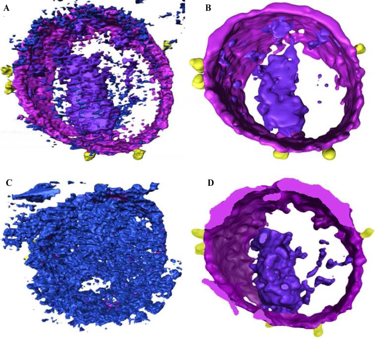
Comparison of feature extraction by manual vs. automated segmentation of dual-axis SIRT reconstructed HIV-1 tomogram. (A) unprocessed and (B) denoised tomogram visualized in the environment of Amira. (C) & (D) Comparison of “single-click” segmentation results for unprocessed and denoised tomograms respectively, with denoising performed using the phase-preserving algorithm.
CONCLUSIONS
Electron tomograms are intrinsically noisy, and this poses significant challenges for image interpretation, especially in the context of low dose and high-throughput data analysis. Our goal has been to evaluate the relative performance of different denoising methods in further improving the SNR, and to test whether these denoised tomograms can be processed automatically to extract biologically relevant information. We show here that denoising significantly improves the fidelity of automated feature extraction. The NAD algorithm performs best for recovering structural information from low-dose cryo tomograms, and spatial information such as ribosome distribution can be obtained automatically from denoised tomograms with results closely matching those obtained using semi-automated approaches. We show that molecular information such as the average volume of individual HIV viral spikes can be obtained from these denoised tomograms, and that the values closely match those obtained using manual user-guided approaches for room temperature tomograms of HIV-1 infected macrophages. The use of these valuable computational tools provides a further step for quantitative analysis of 3D structures determined using electron tomography.
ACKNOWLEDGEMENTS
This work was supported by funds from the intramural program of the National Cancer Institute, NIH, Bethesda, MD. We thank Dr. Alexander Shapiro of the ISYE department and Muhammad Mukarram Bin Tariq of the College of Computing; Georgia Institute of Technology for useful discussion on the GOF tests.
Footnotes
The true noise samples are from the recorded tomograms at room or cryogenic temperatures.
White noise is a random signal (or process) that has a flat power spectral density.
References
- Borgnia M, Subramaniam S, Milne J. Rapid shape variation in the predatory bacterium revealed by cryo-electron tomography. J. Bact. 2008 in press. [Google Scholar]
- Cover TM, Thomas JA. Elements of information theory. Wiley; New York: 1991. [Google Scholar]
- Donoho DL. Denoising via soft-thresholding. IEEE Transactions on Information Theory. 1995;41:613–627. [Google Scholar]
- Fernandez JJ, Li S. An improved algorithm for anisotropic nonlinear diffusion for denoising cryo-tomograms. J Struct Biol. 2003;144:152–61. doi: 10.1016/j.jsb.2003.09.010. [DOI] [PubMed] [Google Scholar]
- Frangakis AS, Forster F. Computational exploration of structural information from cryo-electron tomograms. Curr Opin Struct Biol. 2004;14:325–31. doi: 10.1016/j.sbi.2004.04.003. [DOI] [PubMed] [Google Scholar]
- Frangakis AS, Hegerl R. Noise reduction in electron tomographic reconstructions using nonlinear anisotropic diffusion. J Struct Biol. 2001;135:239–50. doi: 10.1006/jsbi.2001.4406. [DOI] [PubMed] [Google Scholar]
- Frangakis AS, Hegerl R. Segmentation of two- and three-dimensional data from electron microscopy using eigenvector analysis. J Struct Biol. 2002;138:105–13. doi: 10.1016/s1047-8477(02)00032-1. [DOI] [PubMed] [Google Scholar]
- Frangakis AS, Stoschek A, Hegerl R. Wavelet transform filtering and nonlinear anisotropic diffusion assessed for signal reconstruction performance on multidimensional biomedical data. IEEE Trans Biomed Eng. 2001;48:213–22. doi: 10.1109/10.909642. [DOI] [PubMed] [Google Scholar]
- Frank J. Three-Dimensional Electron Microscopy of Macromolecular Assemblies: Visualization of Biological Molecules in Their Native State. Oxford University Press; USA: 2006. [Google Scholar]
- Gilbert P. Iterative methods for the three-dimensional reconstruction of an object from projections. J Theor Biol. 1972;36:105–17. doi: 10.1016/0022-5193(72)90180-4. [DOI] [PubMed] [Google Scholar]
- Gilboa G, Sochen N, Zeevi YY. Image Enhancement and Denoising by Complex Diffusion Processes. IEEE Transactions on Pattern Analysis and Machine Intelligence (PAMI) 2004;26:1020–36. doi: 10.1109/TPAMI.2004.47. [DOI] [PubMed] [Google Scholar]
- Gonzalez RC, Woods RE. Digital Image Processing. Addison-Wesley; Boston, Massachusetts: 1992. http://decsai.ugr.es/~javier/denoise/software/index.htm http://www-stat.stanford.edu/~wavelab/WaveLab701.html http://www.tgs.com/ [Google Scholar]
- Jiang M, Ji Q, McEwen BF. Automated extraction of fine features of kinetochore microtubules and plus-ends from electron tomography volume. IEEE Trans Image Process. 2006;15:2035–48. doi: 10.1109/tip.2006.877054. [DOI] [PubMed] [Google Scholar]
- Jiang W, Baker ML, Wu Q, Bajaj C, Chiu W. Applications of a bilateral denoising filter in biological electron microscopy. J Struct Biol. 2003;144:114–22. doi: 10.1016/j.jsb.2003.09.028. [DOI] [PubMed] [Google Scholar]
- Kovesi P. Phase Preserving Denoising of Images; The Australian Pattern Recognition Society Conference: DICTA'99.1999. pp. 212–217. [Google Scholar]
- Kremer JR, Mastronarde DN, McIntosh JR. Computer visualization of three-dimensional image data using IMOD. J Struct Biol. 1996;116:71–6. doi: 10.1006/jsbi.1996.0013. [DOI] [PubMed] [Google Scholar]
- Moss WC, Haase S, Lyle JM, Agard DA, Sedat JW. A novel 3D wavelet-based filter for visualizing features in noisy biological data. J Microsc. 2005;219:43–9. doi: 10.1111/j.1365-2818.2005.01492.x. [DOI] [PubMed] [Google Scholar]
- Narasimha R, Aganj I, Borgnia M, Sapiro G, McLaughlin S, Milne J, Subramaniam S. From Gigabytes to Bytes: Automated denoising and feature identification in electron tomograms of intact bacterial cells; IEEE International Symposium on Biomedical Imaging (ISBI '07).2007. [Google Scholar]
- Nicastro D, Schwartz C, Pierson J, Gaudette R, Porter ME, McIntosh JR. The molecular architecture of axonemes revealed by cryoelectron tomography. Science. 2006;313:944–8. doi: 10.1126/science.1128618. [DOI] [PubMed] [Google Scholar]
- Nicholson WV, Glaeser RM. Review:automatic particle detection in electron tomography. Journal of Structual Biology. 2001;133:90–101. doi: 10.1006/jsbi.2001.4348. [DOI] [PubMed] [Google Scholar]
- Nicholson WV, Malladi R. Correlation-based methods of automatic particle dtection in electron microscopy images with smoothing by anisotropic diffusion. Journal of Microscopy. 2004;213:119–128. doi: 10.1111/j.1365-2818.2004.01286.x. [DOI] [PubMed] [Google Scholar]
- Nickell S, Mihalache O, Beck F, Hegerl R, Korinek A, Baumeister W. Structural analysis of the 26S proteasome by cryoelectron tomography. Biochem Biophys Res Commun. 2007;353:115–20. doi: 10.1016/j.bbrc.2006.11.141. [DOI] [PubMed] [Google Scholar]
- Pantelic RS, Rothnagel R, Huang CY, Muller D, Woolford D, Landsberg MJ, McDowall A, Pailthorpe B, Young PR, Banks J, Hankamer B, Ericksson G. The discriminative bilateral filter: an enhanced denoising filter for electron microscopy data. J Struct Biol. 2006;155:395–408. doi: 10.1016/j.jsb.2006.03.030. [DOI] [PubMed] [Google Scholar]
- Perona P, Malik J. Scale-space and edge detection using anisotropic diffusion. IEEE Transactions on Pattern Analysis and Machine Intelligence. 1990;12:629–639. [Google Scholar]
- Portilla J, Strela V, Wainwright M, Simoncelli EP. Image Denoising using Scale Mixtures of Gaussians in the Wavelet Domain. IEEE Trans Image Process. 2003;12:1338–1351. doi: 10.1109/TIP.2003.818640. [DOI] [PubMed] [Google Scholar]
- Sandberg K. Methods for image segmentation in cellular tomography. Methods Cell Biol. 2007;79:769–98. doi: 10.1016/S0091-679X(06)79030-6. [DOI] [PubMed] [Google Scholar]
- Sandberg K, Brega M. Segmentation of thin structures in electron micrographs using orientation fields. J Struct Biol. 2007;157:403–15. doi: 10.1016/j.jsb.2006.09.007. [DOI] [PubMed] [Google Scholar]
- Scott DW. Multivariate Density Estimation: Theory, Practice, and Visualization. Wiley-Interscience; New York: 2002. [Google Scholar]
- Subramaniam S, Milne JL. Three-dimensional electron microscopy at molecular resolution. Annu Rev Biophys Biomol Struct. 2004;33:141–55. doi: 10.1146/annurev.biophys.33.110502.140339. [DOI] [PubMed] [Google Scholar]
- Thong JT, Sim KS, Phang JC. Single-image signal-to-noise ratio estimation. Scanning. 2001;23:328–36. doi: 10.1002/sca.4950230506. [DOI] [PubMed] [Google Scholar]
- Weickert J. Anisotropic Diffusion in Image Processing. Teubner-Verlag; Stuttgart, Germany: 1998. [Google Scholar]
- Winkler H. 3D reconstruction and processing of volumetric data in cryo-electron tomography. J Struct Biol. 2007;157:126–37. doi: 10.1016/j.jsb.2006.07.014. [DOI] [PubMed] [Google Scholar]