Boundaries, links and clusters: a new paradigm in spatial analysis?

Abstract

This paper develops and applies new techniques for the simultaneous detection of boundaries and clusters within a probabilistic framework. The new statistic “little b” (written b_ij) evaluates boundaries between adjacent areas with different values, as well as links between adjacent areas with similar values. Clusters of high values (hotspots) and low values (coldspots) are then constructed by joining areas abutting locations that are significantly high (e.g., an unusually high disease rate) and that are connected through a “link” such that the values in the adjoining areas are not significantly different. Two techniques are proposed and evaluated for accomplishing cluster construction: “big B” and the “ladder” approach. We compare the statistical power and empirical Type I and Type II error of these approaches to those of wombling and the local Moran test. Significance may be evaluated using distribution theory based on the product of two continuous (e.g., non-discrete) variables. We also provide a “distribution free” algorithm based on resampling of the observed values. The methods are applied to simulated data for which the locations of boundaries and clusters is known, and compared and contrasted with clusters found using the local Moran statistic and with polygon Womble boundaries. The little b approach to boundary detection is comparable to polygon wombling in terms of Type I error, Type II error and empirical statistical power. For cluster detection, both the big B and ladder approaches have lower Type I and Type II error and are more powerful than the local Moran statistic. The new methods are not constrained to find clusters of a pre-specified shape, such as circles, ellipses and donuts, and yield a more accurate description of geographic variation than alternative cluster tests that presuppose a specific cluster shape. We recommend these techniques over existing cluster and boundary detection methods that do not provide such a comprehensive description of spatial pattern.

1 Introduction

Boundaries of different types have been defined in the literature as zones of rapid change and as the edges of patches, using descriptors such as “open boundaries”, “closed boundaries”, “crisp boundaries”, and “fuzzy boundaries” (Jacquez et al. 2000). While there are many methods for detecting boundaries (Womble 1951; Maruca and Jacquez 2002; Lu and Carlin 2005) and clusters (Besag and Newell 1991; Jacquez et al. 1996; Kulldorff et al. 2005; Patil et al. 2006; Tango 2007), to our knowledge there are not any techniques for simultaneously identifying both boundaries and clusters. The statistics proposed in this paper promise to provide a more complete description of spatial pattern, thereby enabling a comprehensive synthesis of the components of spatial structure (boundaries, links, hotspots and coldspots) that together underlie our cognitive models of geographic variation.

There are two reasons why one would wish to detect the constituents of both boundaries and clusters within one statistical framework. First, there is a duality between boundaries and clusters. Cognitively, the edge of a cluster necessarily implies a boundary, and it thus makes sense when talking about one (e.g., clusters) to recognize and discuss the properties of the other (e.g., boundaries). Second, there is a growing realization among researchers that existing boundary detection and clustering techniques describe highly circumscribed aspects of spatial pattern. Some researchers advocate employing a battery of spatial statistics to better describe several aspects of geographic pattern (Jacquez and Greiling 2003a,b), while others have proposed methods capable of detecting clusters of arbitrary shape (Patil et al. 2006). But to our knowledge ours is the first method to detect both boundaries and clusters at once.

Commonly used disease clustering methods are often based on unrealistic assumptions. There is a growing awareness that clusters can take on a variety of different shapes, yet most commonly used clustering methods are sensitive to only one shape (Jacquez 2004; Tango and Takahashi 2005; Kulldorff et al. 2006). For example, the scan statistics currently available in the widely-used SatScan software assume under the alternative hypothesis that clusters are shaped as circles or ellipses, and hence these tests hence have reduced power to detect other, more realistic, configurations. Similarly, LISA statistics (Ord and Getis 1995) use pre-defined neighborhoods such as 1st order adjacencies, 2nd order adjacencies and so on, and are less sensitive to clustering that occurs for different shapes or at different spatial scales (Greiling et al. 2005). Other techniques, such as kernel-based methods, necessarily involve smoothing that can “wash out” spatial heterogeneity by averaging within the chosen kernel. While these deficiencies are now widely acknowledged, techniques that accurately identify clusters of arbitrary shape are just now being developed.

This paper develops and applies a new technique for the simultaneous detection of boundaries, clusters and links between similar adjacent areas. The approach is “distribution free” in the sense that randomization is used to evaluate statistical significance, and it also is “geographic template free” in the sense that it is not constrained to find clusters of a pre-specified shape, such as circles, ellipses, donuts and etc. Since this new approach relaxes the assumption of a specific cluster shape that underpins almost all existing cluster tests, and describes boundaries as well as clusters, we believe it yields a more accurate description of geographic patterns.

This paper focuses on the analysis of disease rates, but the reader will please appreciate the technique is generally applicable to variables with continuous distributions or to discrete variables (e.g., counts) with a sufficient number of observations so that they can in practice be treated as continuous. The technique as currently framed is not appropriate for binary data such as case–control identifiers.

2 Methods

The Methods section first defines notation and then introduces the b-statistic (little b) for detection of boundaries and links, the B-statistic (big B) for the detection of hotspots and cold-spots, and a map logic approach (called ladder) for cluster construction. The b-scattergram is defined, followed by randomization- and distribution-based approaches for evaluating statistical significance. The simulation design is then presented, along with the risk model used in the simulation study. Finally, we define the statistics used for assessing map classification, Type I error, Type II error, statistical power, sensitivity and specificity.

2.1 Notation

Suppose you observe the value of some variable x at N point locations or areas on a map. For simplicity of exposition we assume for the remainder of this paper that we are working with areas (e.g., polygons such as counties). Denote the value for area i as x_i. The variable x is a continuous variable with unknown distribution. Again, for purposes of exposition, let us assume x is a mortality rate such as the lung cancer mortality rate in a county. This rate can be transformed into a standardized deviate with zero mean as:

$$z_i=\frac{x_i-{\overline{x}}_{H0}}{s_x}.$$ (1)

Here x̄_H0 is the mean of x under the null hypothesis (e.g., the background rate) and s_x is its standard deviation, again under the null hypothesis.

2.2 The b-statistic for detection of boundaries and links

The b-statistic for the pair of areas i and j is defined as:

$$\begin{array}{l}{b}_{ij}=w_{ij}{z}_i{z}_j\\ w_{ij}=\{\begin{array}{ll}1\hfill & \text{if}\text{areas}i\text{and}j\text{have}\text{a}\text{common}\text{border}\hfill \\ 0\hfill & \text{otherwise}.\hfill \end{array}\end{array}$$ (2)

The weights w_ij are binary and indicate whether or not areas i and j are adjacent. Little b is thus simply the product of the two z-scores observed in a pair of geographically adjacent areas. Unlike LISA statistics such as the local Moran, G and G*, which describe local spatial variation in the immediate local neighborhood about a central location, the b-statistic describes properties of the edge between areas i and j. Here, large negative b_ij values mean z_i and z_j are very different, positive b_ij mean both z_i and z_j are negative (cold) or both z_i and z_j are positive (hot). Hence the b-statistic is used for evaluating the edges between location pairs to define them as either links between similar high or low areas (e.g., cluster constituents), or boundaries between two dissimilar areas. We will continue to use the word “link” to describe an edge separating two similar areas that are to be joined together, and “boundary” to describe the edge between two areas that are different from one another. Unlike wombling, which requires the definition of arbitrary thresholds for evaluating boundary significance, the probability of the b-statistic may be evaluated using either distribution theory or randomization, as described next. This illustrates an important advantage of b-statistics relative to wombling: Arbitrary thresholds regarding boundary magnitude are not required.

2.3 The b-scattergram

By analogy with the Moran scatterplot or the h-scattergram used in geostatistics, a b-scattergram can be created by plotting the value for the ith location (e.g., z_i) on the x-axis and the value of the neighbor (e.g., z_j) on the y-axis (Fig. 1). The intersection of the x and y axes is 0,0 resulting in 4 quadrants: z_i and z_j > 0 (HH link); z_i and z_j < 0 (LL link); z_i > 0 and z_j < 0 (HL boundary); z_i < 0 and z_j > 0 (LH boundary). One then evaluates the significance of links connecting adjacent areas of high or low values to create larger high or low clusters, and the significance of boundaries that correspond to large negative values of the b-statistic. The b-scattergram illustrates the importance of transformation to a space in which the z are sampled from a distribution with both positive and negative values. As shown in Eq. 1, this transformation may reflect the null hypothesis or “neutral model” (Goovaerts and Jacquez 2004) being explored. Goovaerts and Jacquez (2004) offered a typology of neutral models based on whether or not the null spatial model assumed a spatially uniform mean, a geographically heterogeneous population density and/or spatial autocorrelation in the variable under scrutinity. For example, when exploring the possible existence of clusters defined a priori, one could set x̄_{H 0} to be the mean rate observed in those areas not including the a priori cluster (e.g., the background), and to incorporate that level of spatial autocorrelation expected in the absence of a cluster process.

Fig. 1.

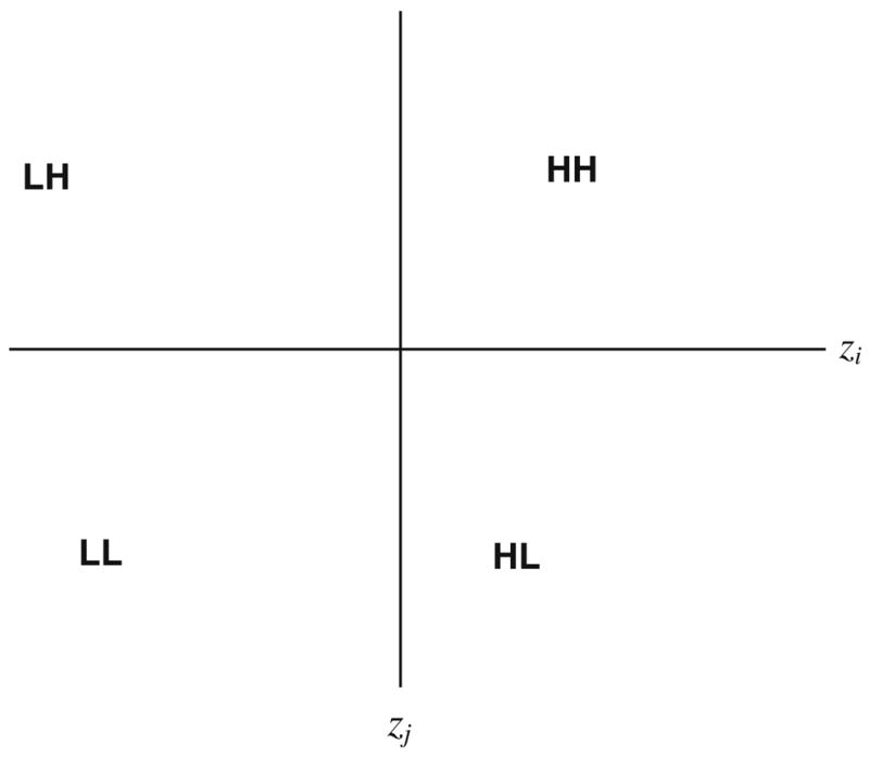
The b-scatterplot

2.4 Significance under randomization

The distribution of b_ij may be evaluated using distribution theory or distribution-free randomization, depending on whether or not z may be assumed to be spatially independent. When the z_i, z_j are assumed independent under the null hypothesis, distribution theory¹ may be used to evaluate the statistical significance of the b-statistic, as discussed later. When this assumption does not hold it is convenient to use conditional randomization to evaluate probabilities. Here we consider two cases: spatial independence of the z_i, z_j (Case 1) and z_i, z_j spatially autocorrelated (Case 2).

Case 1: Spatial independence of z_i, z_j

In this instance distribution theory and randomization should yield highly similar results. A conditional randomization is used to evaluate the significance of an observed b_ij statistic, denoted $b_{ij}^{\ast }$. Conditional randomization occurs when the value of z_i is held constant and one samples from the vector of (N − 1)z values to select a value for z_j. The randomization is said to be conditional because the observed value of z_i is associated with area i under each such realization. One then calculates the value of b_ij for each realization to construct a reference distribution of b_ij under the null hypothesis of spatial independence. When evaluating the clustered alternative (e.g., a HH link or a LL link), the probability under this null hypothesis of observing a b_ij as large as or larger than the observed $b_{ij}^{\ast }$ is

$$P(b_{ij}\ge b_{ij}^{\ast }\mid H_0)=\frac{a+1}{c+1}.$$ (3)

Here a is the number of realizations for which $b_{ij}\ge b_{ij}^{\ast }$, and c is the total number of realizations conducted. The lower left tail of the reference distribution is used when considering the boundary alternative (e.g., HL or LH boundary) and one calculates the probability of b_ij being as small or smaller than $b_{ij}^{\ast }$:

$$P(b_{ij}\le b_{ij}^{\ast }\mid H_0)=\frac{d+1}{c+1}.$$ (4)

Here d is the number of realizations for which $b_{ij}\le b_{ij}^{\ast }$. This approach is useful when the null hypothesis of spatial independence of the z values is reasonable. However, as for all randomization techniques that resample the observed data, the scope of inference is limited to the observed data set.

Case 2: z_i, z_j are not independent

In this situation one can not use the randomization approach under Case 1 nor the distribution theory outlined below because the assumption of independent z_i, z_j does not hold. One then uses the typology of neutral models of Goovaerts and Jacquez (2004), and the randomization approaches they define that account for spatial autocorrelation under the null hypothesis. This allows one to account for a specified level of spatial autocorrelation under the null hypothesis, as well as a geographically varying background rate. The b_ij that are found significant are statistically unusual under the model of the underlying risk that is specified by the neutral model. In this paper we only evaluate statistical significance using Case 1, spatial independence. We recognize that this in practice is highly unrealistic but employ it as a first step in the evaluation of this new approach. Future research will incorporate more realistic neutral models to specify geographic variation in risk under the null hypothesis.

2.5 Significance under distribution theory

What is the distribution of the product of two random variables? Craig (1936), derived the algebraic form of the moment-generating function of the product of two Gaussian variables. Aroian (1947) provides the probability function for the product of two normally distributed variables. When the mean is zero, the probability density function or pdf of the product of two Gaussian random variables is the Bessel function. Ware and Ladd (2003) provide the moment-generating function of the product of two correlated normally distributed variables. Glen et al. (2004) provide algorithms for computing the distribution of the product of two continuous random variables and consider both independent and correlated cases. Specifically, they consider the continuous random variables X and Y with joint pdf f_X,Y (x, y). The pdf of the product V =XY as attributed to Rohatgi (1976, p. 141) is

$$f_V(v)=\underset{-\infty }{\overset{\infty }{\int }}{f}_{X,Y}(x,\frac{v}{x})\frac{1}{\mid x\mid }dx.$$ (5)

This is difficult to implement as an algorithm, and Glen et al. (2004) offer several approaches for special cases of X and Y, including their example 4.3, X ~ N(0,1) and Y ~ N(0,1); X and Y independent.

When working with relatively small data sets it is computationally straightforward to employ randomization approaches that can assume either independent or spatially correlated variables. In the results presented later we use conditional randomization assuming independence. As noted earlier, when the observations are not independent one can use the neutral models technique for spatially correlated variables with either uniform or non-uniform risk (Goovaerts and Jacquez 2004).

2.6 Cluster evaluation

Having considered how the statistical significance of little b may be evaluated we complete the definition of the approach by presenting two ways of constructing clusters. The first, called big B, seeks to define hotspots and cold spots using the b_ij themselves. The second, called “ladders”, use the Poisson probabilities of the underlying rates and the statistical significance of the links to create clusters of high and low rates.

3 Constructing clusters using big B

Let k denote the number of objects (e.g., counties) that are adjacent to area i, i.e. the set of areas with w_ij = 1. The B-statistic (“big B”) is defined as the following ordered tuple:

$$B_i=\{b_{i1},b_{i2},\dots ,b_{ik}\}.$$ (6)

The statistical significance of big B is evaluated under randomization by generating m ordered tuples of the form $B_i^{\prime }=\{b_{i1}^{\prime },b_{i2}^{\prime },\dots ,b_{ik}^{\prime }\}$. The randomization is accomplished by holding the ith value, z_i, fixed, drawing a random sample of size k from the remaining (N − 1) z_j and assigning these to the k adjacent areas. The $b_{ij}^{\prime }$ for j = 1 up to k are then calculated to define a $B_i^{\prime }$ under conditional randomization. The centroid of the set of m simulated tuples $B_i^{\prime }$ is computed in the k-space and the Euclidian distance between this centroid and each individual tuple is calculated. The same procedure is followed for the observed tuple B_i and the observed Euclidian distance is compared to the empirical distribution of m simulated distances. Observed distances that are larger than most of the simulated ones indicate presence of clusters, that is a group of consistently positive observed b-statistics. In our simulation study this statistic did not perform as well as the ladder approach (below). Areas which have very high values do not end up being significant under randomization but their moderately high neighbors do, leading to an increase in both Type I and Type II errors. This may be caused when moderately high values adjacent to very high-valued neighbors are swapped out the result is a much lower value, but when the neighbors of the very high-valued object are swapped out the effect is not as great. This led us to formulate the ladder approach to constructing clusters.

4 Constructing clusters using ladders

Recall that positive b_ij values correspond to a link between adjacent high areas (a HH link) or between adjacent low areas (a LL link). When working with disease rates public health professionals are concerned primarily with identifying clusters comprised of significant high or low rates. We propose a multi-step approach to constructing clusters and illustrate it for clusters of high values (an analogous approach is used to construct clusters of low values). First, we identify those areas whose observed rates (x_i) or counts are statistically higher than what would be expected according to a Poisson distribution. Here the expected number of cases is calculated as the mean rate under the null hypothesis (x̄_H0) multiplied by the population at risk in area i. Second, areas whose Poisson P values are less than the desired significance level (e.g., 0.05) are identified and used to construct the set of seed areas for cluster growth. These seed areas are then each considered in turn, and are connected to other adjacent areas with which a HH link is shared to construct larger clusters. Adjacent areas that have been included in a cluster are then considered, and their neighbors also are included in the cluster if they are connected to the growing cluster with a HH link. The cluster growth process stops when no more areas may be added through HH links. This results in clusters of high values with arbitrary shape that always contain at least one area whose rate is statistically significant under the Poisson distribution. Outliers may be considered by allowing clusters to consist of only one member—an area has a significantly high rate but is not joined to any of its neighbors by HH links.

To summarize, the step-by-step procedure for constructing clusters using the ladder approach is as follows.

1. Identify areas that are significantly high or low. For example, when working with disease rates one would evaluate the significance of a given rate using the Poisson distribution for the size of the at risk population in that area. Each of these significantly high or low areas is referred to as a “seed”.

2. Considering each seed in turn, deem an adjacent area to be part of the cluster only when it is connected to the seed by a HH link (for a high cluster) or a LL link (for a low cluster). The contiguous area formed by connecting the seed through the HH links (or LL links when considering cold spots) is the spatial extent of the cluster.

3. Continuing growing the cluster by repeating Step 2 as the cluster grows, until no additional areas can be added to the cluster through adjacent HH or LL links.

4.1 Simulation study

We employed simulated data sets for which the locations of clusters and boundaries are known in order to provide a controlled experimental setting. We compared the boundary detection capabilities of the b_ij statistic to that of polygon wombling (Maruca and Jacquez 2002). We also compared the cluster detection capabilities of the big B and ladder approaches to that of the local Moran statistic. We now briefly present each of these statistics. The reader who is not already familiar with these techniques may wish to read the details in the cited literature.

In polygon wombling a difference measure is calculated across each candidate boundary element, which is defined as a boundary separating two adjacent areas. The value so calculated is called a BLV or Boundary Likelihood Value, and its statistical significance is evaluated through randomization, e.g. 9999 randomizations in our analyses that were conducted using the BoundarySeer software from TerraSeer Inc.

The local Moran test evaluates local clustering or spatial autocorrelation. Its null hypothesis is that there is no association between rates in neighboring areas. The working (alternative) hypothesis is that spatial correlation exists; either with a positive sign (cluster) or a negative one (outlier). The local Moran statistic is calculated as the product of the value for the area being considered (kernel) and the average value for all of its surrounding neighbors. As for the b-statistic, the values are first standardized to a zero mean. A negative value for the local Moran statistic thus indicates a negative local autocorrelation and the presence of spatial outlier where the kernel value is much lower or much higher than the surrounding values. Cluster of low or high values will lead to positive values of the statistic. The local Moran analysis was conducted using TerraSeer’s Space Time Intelligence System (STIS) software.

5 Study design

We first constructed a risk model using a realistic geography (counties in Michigan) for which the risk function was specified by the researcher. We based our model on pancreatic cancer mortality for white males observed from 1970 to 1994. For the background risk in the model we used the state-wide pancreatic cancer mortality for white males per 100,000 (age standardized). This yielded a background rate of 9.57 deaths per 100,000. We next constructed two clusters, one in the north and one in the south, each comprised of five counties (Fig. 2, left). The relative risk in the northern cluster was 2.0, and for the south 1.5. For the geographic distribution of the at-risk population, we used the age-standardized at-risk population for white male pancreatic cancer (Fig. 2, center) from the STIS for the National Atlas of Cancer Mortality (http://www.biomedware.com/software/Atlas_download.html). We then simulated a realization of this risk surface by sampling from the modeled mean as a Poisson process and using the population size in each area. This resulted in a realization of the risk model whose spatial variance is a function of geographic heterogeneity in the at-risk population (Fig. 2, right).

Fig. 2.

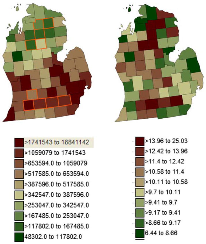
Population distribution is the age-adjusted at risk population for pancreatic cancer in white males, 1970–1994 (left). North and south clusters are outlined in gold (left). One realization of the disease simulation (right)

6 Methods comparison

We analyzed the realization from the simulation using alternative boundary (polygon wombling) and cluster analysis (local Moran) methods, and compared the results from these techniques to the corresponding b-statistic. To accomplish this comparison we first quantified the accuracy of each method using a classification table:

		Found
		Boundary	No boundary
Truth	Boundary	a	b
	No boundary	c	d.

This illustrates a classification table for evaluation of boundary detection methods; similar ones were constructed for evaluation of the cluster detection methods. Two were created for the boundary analysis methods (polygon wombling, little b) and 3 were created for the clustering methods (Big B, ladder, LISA). Suppose we are evaluating the accuracy of polygon wombling. Entry a would be a count of the number of true boundaries that were correctly found to be boundaries; b would be the number of true boundaries that were incorrectly identified as not being boundaries (a false negative), c is the number of borders that were mistakenly identified as boundaries (a false positive), and d is the number of borders that are not boundaries and were correctly identified as such. From these counts we then calculate the following statistics.

Number of boundaries = a + b:	36
Number of not boundaries = c + d:	117
Specificity = a/(a + b)
Empirical Type I error = b/(a + b)	(α)
Empirical Type II error = c/(c + d)	(β)
Power or sensitivity = d/(c + d)	(1 − β)

7 Results

Histograms of the modeled and simulated rates show that substantial noise was introduced through the Poisson sampling process (Fig. 3). In this preliminary research we only analyzed one such realization of the Poisson process. Future research will expand the scope of the simulations but it is sufficient in this preliminary analysis to try out the simulation design and to evaluate whether the new b-statistics have any characteristics that are desirable relative to existing methods.

Fig. 3.

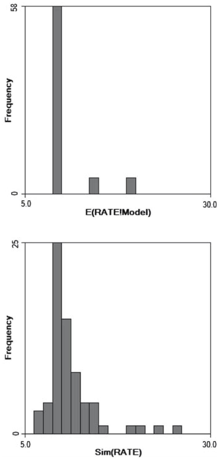
Histogram of mortality rates under the model (top) and after sampling the modeled risk as a Poissson process (bottom). Noise introduced in this fashion is proportional to the size of the at-risk population

Polygon wombling versus Little b

Figure 4 shows the results obtained when polygon wombling and little b are applied to the modeled risk and to the simulated surfaces. Both methods found all boundaries for the model, although the Womble approach could not identify significant links (it is not designed to do so). When noise is introduced in the simulation the Womble approach missed more true boundaries, but the b-approach incorrectly classified two edges as boundaries. These results are summarized in Tables 1, 2.

Fig. 4.

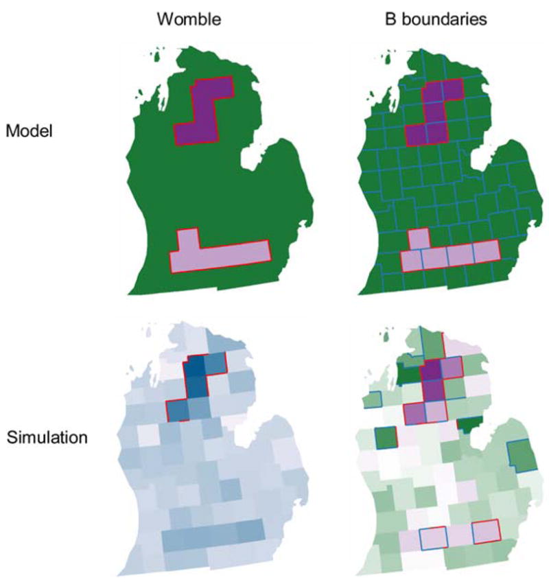
Womble (left column) and boundary analysis using little b (right column) for the modeled risk surface (top row) and realization of that surface as a Poisson process (bottom row). Red lines indicate statistically significant boundaries, blue lines indicate significant links between areas of similar values. Both methods found all boundaries for the model, although the Womble approach could not identify significant links. When noise is introduced in simulation the Womble approach missed more true boundaries, but the b-approach misidentified two edges as boundaries

Table 1.

Counts of edge classification results

	b-Statistic				Polygon Womble
	a	b	c	d	a	b	c	d
Model	36	0	0	117	36	0	0	117
Simulation	21	15	4	113	12	24	0	117

Table 2.

Accuracy and error statistics for boundary classification using the little b and polygon wombling approaches

	b-Statistic				Polygon Womble
	Specificity	Type I	Type II	Power	Specificity	Type I	Type II	Power
Model	1.000	0.000	0.000	1.000	1.000	0.000	0.000	1.000
Simulation	0.583	0.417	0.034	0.966	0.333	0.667	0.000	1.000

The Little b approach has a substantially greater specificity (0.583 vs. 0.333) and smaller type I error (0.417 vs. 0.667) than polygon wombling. This occurs at the expense of a slight increase in Type II error (0.034 vs. 0.000) and a small drop in statistical power (0.966 vs. 1.000). In addition, the little b approach is able to identify links that can then be used in the ladder approach to construct clusters. For the highly limited scope of inference of this simulation study, little b has outperformed polygon wombling in terms of its ability to accurately detect boundaries.

Big B and Ladders versus Local Moran

We also compared and contrasted the hot and cold clusters found under the big B, Ladder and Local Moran approaches. Figure 5 shows the findings from these approaches, and the results differ markedly from one method to another. Surprisingly, the local Moran technique was unable to identify the true clusters even for the modeled data when noise was absent. This failure most likely is due to its geographic template, which averages across all of the neighbors of each individual county. It thus has poor ability to detect clusters that are not comprised of all of an areas’ adjacent neighbors. These results are summarized in Tables 3, 4.

Fig. 5.

Results of the analysis of the modeled (top row) and simulated data (bottom row) for the big b (first column), ladder (second column) and local Moran (third column) approaches. Only the Ladder approach correctly detected both the north and south clusters in both the model and simulation surfaces, but at the expense of several false positives

Table 3.

Counts from classification table for Big B, Ladder and Local Moran methods

	Big B				Ladder				Local Moran
	a	b	c	d	a	b	c	d	a	b	c	d
Model	5	5	6	70	10	0	0	76	2	8	7	69
Simulation	4	6	5	71	10	0	4	72	4	6	6	70

Table 4.

Specificity, Type I and Type II error, and sensitivity of the Big B, Ladder and Local Moran methods

	Big B				Ladder				Local Moran
	Specificity	Type I	Type II	Power	Specificity	Type I	Type II	Power	Specificity	Type I	Type II	Power
Model	0.500	0.500	0.079	0.921	1.000	0.000	0.000	1.000	0.200	0.800	0.092	0.908
Simulation	0.400	0.600	0.066	0.934	1.000	0.000	0.053	0.947	0.400	0.600	0.079	0.921

For the risk model the Ladder approach is the only one to make the correct inference as being part of a cluster, or not being part of a cluster, 100% of the time. Big B found an area to actually be part of a true cluster only 50% of the time, while the local Moran made this correct decision only 20% of the time. In a more realistic situation where noise attributable to finite population size is included in the simulation, the Ladder approach still correctly identified clusters with 100% accuracy. However, it also deemed non-clusters to be part of a cluster 5.3% of the time. By comparison, the local Moran and Big B approaches correctly found true clusters only 40% of the time, and incorrectly declared a county at background to be part of the cluster 6.6% of the time (Big B) and 7.9% of the time (local Moran). For cluster detection, the ladder approach is superior to both Big B and local Moran.

8 Discussion and conclusion

We compared our new statistics only to the Womble and local Moran techniques, although dozens of alternative methods are available. Comparison to certain techniques, such as the join count method, would not be appropriate, since the join-count statistics work with categorical data, while our methods are designed for continuous data. Csillag et al. (2001) proposed techniques for multiscale characterization of boundaries that work across edge-pairs, much as the b-statistic proposed in this paper. The methods differ in that Csillag et al. calculate differences across edges, while we calculate the product of the standardized z-scores. We have yet to compare the performance of our b-statistics to the techniques of Csillag et al.

When we consider this body of results it is clear that the little b approach gives comparable results to polygon wombling when detecting boundaries, and that the ladder approach is superior to both Big B and the local Moran statistic for accurately detecting clusters. It must be emphasized that these results are very limited in the scope of their inference. We analyzed only one risk geography comprised of two clusters, and for that geography analyzed only one realization from the risk surface. We thus are not able to make statements regarding the impact of sampling fluctuations on our estimates for specificity, Type I and Type II error, and statistical power. That will require a larger study where we analyze suites of simulated surfaces.

In addition, we have not considered other geographic scales nor geographies from different areas. For example, might this pattern of results hold for census-level geography in Iowa where edge effects are not as strong and for which population heterogeneity is reduced? Finally, we considered pancreatic cancer mortality as our model, a cancer that accounts for the 5th or 6th most cancer deaths depending on gender, age group and geographic region being considered. What if we had used a rare cancer such as cancers of the brain and central nervous system? Rates for such cancers would be even more unstable than pancreatic cancer, due to the small numbers problem. We have yet to definitively evaluate how the little b and ladder approaches behave as uncertainty in the underlying rates increases.

Our risk model in certain respects is unrealistic. While we used a background rate estimated for a representative real cancer (pancreatic cancer in white males) and employed an observed population distribution for the at-risk population, we assumed the background risk was uniform outside of the clusters. Also, within clusters we assumed the risk was uniform, being either relative risk (RR) = 2.0 for the northern cluster or RR = 1.5 for the southern cluster. Our specification of cluster size (5 counties) and shape also was entirely arbitrary. Future simulations studies are needed to explore how relative risk models, cluster size and cluster shape might impact the results.

Despite the limitations inherent in the simulation study design, we are able to conclude that in this one well defined case, that is somewhat realistic in that it used a real geography (counties in Michigan), an observed population distribution (at-risk population for white males in those counties) and a known disease rate for the background (pancreatic cancer mortality rate in Michigan 1970–1994), the little b and ladder statistics are as good as or better than the polygon wombling and local Moran alternatives. Further, because the b-statistics evaluate boundaries, links, hotspots and cold-spots simultaneously, they hold the promise of a more detailed and comprehensive description of geographic variation than is currently available in any other method. While more work is needed to explore the behavior of this new technique, it appears at this point to be a potentially viable and powerful alternative to some existing methods.

In conclusion, this paper developed and applied a new technique for the simultaneous detection of boundaries, clusters and links between similar adjacent areas. The approach is “distribution free” in the sense that randomization is used to evaluate statistical significance, and it also is “geographic template free” in the sense that it is not constrained to find clusters of a pre-specified shape, such as circles, ellipses, donuts and etc. Because this new approach relaxes the assumption of a specific cluster shape that underpins almost all existing cluster tests, we believe it yields a more accurate description of geographic variation in disease patterns. It is to be preferred over existing methods that employ circles, ellipses and other unrealistic shapes to specify the alternative hypothesis under clustering.

Biographies

Geoff M. Jacquez is president and founder of BioMedware, Inc., where he conducts research on the space-time analysis of disease patterns in relation to risk factors and environmental exposures. He is also an adjunct associate professor of environmental health sciences at The University of Michigan in Ann Arbor. Dr. Jacquez’s research interests include exposure reconstruction and the statistical analysis of health–environment relationships for mobile individuals.

Andy Kaufmann is senior software engineer with BioMedware Inc., where he programs space-time intelligence system (STIS) software and methods. His research interests include the development of computer algorithms for the statistical analysis of health–environment relationships accounting for spatial and temporal dependencies.

Pierre Goovaerts is chief scientist with BioMedware Inc. where he conducts NIH funded research on the development of geostatistical methodology for the analysis of health and environmental data. He is also a courtesy associate professor with the Soil and Water Science Department, University of Florida, Gainesville. Dr. Goovaerts has authored more than 80 refereed papers in the field of theoretical and applied geostatistics, including the 1997 textbook “Geostatistics for Natural Resources Evaluation”.

References

- Aroian LA. The probability function of a product of two normally distributed variables. Ann Math Stat. 1947;18:265–271. [Google Scholar]
- Besag J, Newell J. The detection of clusters in rare diseases. J Roy Stat Soc Ser A. 1991;154:143–155. [Google Scholar]
- Craig CC. On the frequency function of xy. Ann Math Stat. 1936;7:1–15. [Google Scholar]
- Csillag C, Boots B, Fortin M-J, Lowell K, Potvin F. Multiscale charaterization of boundaries and landscape ecological patterns. Geomatica. 2001;55:291–307. [Google Scholar]
- Glen AG, Leemis LM, Drew JH. Computing the distribution of the product of two continuous random variables. Comput Stat Data Anal. 2004;44:451–464. [Google Scholar]
- Goovaerts P, Jacquez GM. Accounting for regional background and population size in the detection of spatial clusters and outliers using geostatistical filtering and spatial neutral models: the case of lung cancer in Long Island, New York. Int J Health Geogr. 2004;3:14. doi: 10.1186/1476-072X-3-14. [DOI] [PMC free article] [PubMed] [Google Scholar]
- Greiling DA, Jacquez GM, Kaufmann AM, Rommel RG. Space time visualization and analysis in the Cancer Atlas Viewer. J Geogr Syst. 2005;7:67–84. doi: 10.1007/s10109-005-0150-y. [DOI] [PMC free article] [PubMed] [Google Scholar]
- Jacquez GM. Current practices in the spatial analysis of cancer: flies in the ointment. Int J Health Geogr. 2004;3:22. doi: 10.1186/1476-072X-3-22. [DOI] [PMC free article] [PubMed] [Google Scholar]
- Jacquez GM, Greiling DA. Geographic boundaries in breast, lung and colorectal cancers in relation to exposure to air toxics in Long Island, New York. Int J Health Geogr. 2003a;2:4. doi: 10.1186/1476-072X-2-4. [DOI] [PMC free article] [PubMed] [Google Scholar]
- Jacquez GM, Greiling DA. Local clustering in breast, lung and colorectal cancer in Long Island, New York. Int J Health Geogr. 2003b;2:3. doi: 10.1186/1476-072X-2-3. [DOI] [PMC free article] [PubMed] [Google Scholar]
- Jacquez GM, Waller LA, Grimson R, Wartenberg D. The analysis of disease clusters, Part I: state of the art. Infect Control Hosp Epidemiol. 1996;17:319–327. doi: 10.1086/647301. [DOI] [PubMed] [Google Scholar]
- Jacquez GM, Maruca SL, Fortin MJ. From fields to objects: a review of geographic boundary analysis. J Geogr Syst. 2000;2:221–241. [Google Scholar]
- Kulldorff M, Heffernan R, Hartman J, Assuncao R, Mostashari F. A space-time permutation scan statistic for disease outbreak detection. PLoS Med. 2005;2:e59. doi: 10.1371/journal.pmed.0020059. [DOI] [PMC free article] [PubMed] [Google Scholar]
- Kulldorff M, Huang L, Pickle L, Duczmal L. An elliptic spatial scan statistic. Stat Med. 2006;25(22):3929–3943. doi: 10.1002/sim.2490. [DOI] [PubMed] [Google Scholar]
- Lu H, Carlin BP. Bayesian areal wombling for geographical boundary analysis. Geogr Anal. 2005;37(3):265–285. [Google Scholar]
- Maruca SL, Jacquez GM. Area-based tests for association between spatial patterns. J Geogr Syst. 2002;4:69–84. [Google Scholar]
- Ord J, Getis A. Local spatial autocorrelation statistics: distributional issues and an application. Geogr Anal. 1995;27:286–306. [Google Scholar]
- Patil GP, Modarres R, Myers WL, Patankar AP. Spatially constrained clustering and upper level set scan hotspot detection in surveillance geoinformatics. Environ Ecol Stat. 2006;13(4):365–377. [Google Scholar]
- Rohatgi VK. An introduction to probability theory and mathematical statistics. John Wiley & Sons; New York: 1976. [Google Scholar]
- Tango T. A class of multiplicity-adjusted tests for spatial clustering based on case-control point data. Biometrics. 2007;63:119–127. doi: 10.1111/j.1541-0420.2006.00633.x. [DOI] [PubMed] [Google Scholar]
- Tango T, Takahashi K. A flexibly shaped spatial scan statistic for detecting clusters. Int J Health Geogr. 2005;4:11. doi: 10.1186/1476-072X-4-11. [DOI] [PMC free article] [PubMed] [Google Scholar]
- Ware B, Ladd F. Approximating the distribution for sums of products of normal variables. University of Canterbury Mathematics and Statistics Department; 2003. [Google Scholar]
- Womble WH. Differential systematics. Science. 1951;114:315–322. doi: 10.1126/science.114.2961.315. [DOI] [PubMed] [Google Scholar]