When Fit Indices and Residuals Are Incompatible

Abstract

Standard chi-square-based fit indices for factor analysis and related models have a little known property: They are more sensitive to misfit when unique variances are small than when they are large. Consequently, very small correlation residuals indicating excellent fit can be accompanied by indications of bad fit by the fit indices when unique variances are small. An empirical example of this incompatibility between residuals and fit indices is provided. For illustrative purposes, an artificial example is provided that yields exactly the same correlation residuals as the empirical example but has larger unique variances. For this example, the fit indices indicate excellent fit. A theoretical explanation for this phenomenon is provided using relationships between unique variances and eigenvalues of the fitted correlation matrix.

When assessing structural equation models, it is helpful to use a fit index as a single summary measure and to also inspect the matrix of residual covariances or correlations in case it suggests sources of lack of fit. In the hypothetical situation in which a model holds exactly, the chi-square goodness-of-fit statistic, on which standard fit indices are based, will have a value of zero and all residuals will also be zero (e.g., Bollen, 1989, p. 263). It is tempting to assume, therefore, that the standard fit indices and the usual residuals measure lack of fit of a structural equation model in a compatible manner. In this article, we show that this assumption is not true, particularly when the model fits closely, but not exactly, and when unique variances of manifest variables are very small. Small unique variances imply that both the error variances and specific variances of manifest variables are small so that the manifest variables yield accurate measures of the latent variables under consideration. It is disturbing that standard fit indices appear to indicate a bad fit by the model when very accurate measurements are used and even when all the residuals indicate a very good fit.

This anomaly is examined in some detail. First, a numerical illustration of the problem is given. A matrix of correlations among eight variables from an empirical study in health psychology is subjected to an exploratory maximum-likelihood (ML) factor analysis extracting two factors. Values of several standard fit indices indicate an unsatisfactory fit. The usual residual correlation matrix is then presented. Elements are all small in magnitude, indicating a very good fit of the model and contradicting the fit indices. This illustrates that serious conflicts between the standard fit indices and the correlation residuals can occur in practice.

An artificial correlation matrix, also with eight variables, is then presented. When this correlation matrix is factor analyzed by ML extracting two factors, exactly the same residuals are obtained as in the empirical study. Unique variances, however, are larger for the artificial example than for the empirical example. The fit indices now indicate a very good fit of the model, thereby agreeing with the residuals. Thus, ML factor analyses of two different correlation matrices result in exactly the same residuals but yield fit indices that indicate a very poor fit when some unique variances are small and an excellent fit when they are larger.

A theoretical explanation for this phenomenon is given. It is shown that fit indices based on the chi-square test of fit are influenced by eigenvalues of the fitted, or implied, correlation matrix as well as by the residuals. These fit indices therefore contain information not present in the correlation residuals and are consequently not entirely compatible with them. The incompatibility is most striking when some of the eigenvalues are very small. Because no eigenvalue can be smaller than the smallest unique variance, severe incompatibility of fit indices and residuals cannot occur when no unique variances are small. Transformed residuals that incorporate information about the fitted correlation matrix are then suggested. Chi-square-based fit indices can be calculated directly from the transformed residuals, also using sample size, number of variables, and degrees of freedom. Because the transformed residuals contain all additional information required by the fit indices and not present in the usual residuals, they may be regarded as entirely compatible with the fit indices.

In some situations (but not all; see Costner & Schoenberg, 1973), the usual residuals may be used to locate sources of lack of fit of the model. Comparisons of the transformed residuals and the usual residuals obtained in the two examples are made. The transformed residuals exhibit similar patterns to those of the usual residuals but differ in magnitude. Thus the transformed residuals reflect the magnitude of the standard fit indices. The relative magnitude of the transformed residuals should also provide information for locating sources of lack of fit in situations in which this is possible with the usual residuals.

The findings about the influence of small unique variances on the magnitude of the chi-square test statistic are shown to have implications for the power of the chi-square test of fit. Effect size will be large, and consequently power will be high, when the manifest variables used have small unique variances.

Incompatible fit indices and residuals occur only in the presence of small unique variances. Because highly accurate measurements are seldom available in the social sciences, this incompatibility is not often obvious in practice. Obvious incompatibilities do, however, sometimes occur, particularly in experimental contexts in which closely related or repeated biologic, physical, or other highly reliable measurements are collected. Steiger (2000, pp. 160–161) has commented independently on this problem, and colleagues have, on occasion, been very puzzled by the phenomenon and consulted some of us. These puzzled consultations have provided the impetus for the present article.

An Illustrative Example

The data come from a clinical trial of the efficacy of a psychological intervention to reduce stress, enhance quality of life, improve health behaviors, and enhance biologic responses for women with breast cancer (Andersen et al., 1998; Andersen, Kiecolt-Glaser, & Glaser, 1994). One focus of this work was on biologic responses to the intervention, specifically, the response of the immune system. In the present analyses, we make use of two immune measures: natural killer (NK) cell lysis (cytotoxicity) and the response of NK cells to recombinant interferon gamma (rIFNγ). Higher levels of these variables indicate a stronger response of the immune system. For each measure, the corresponding laboratory assay was conducted with four replicates, differing in terms of the ratios of effector to target (E:T) cells. For NK cell lysis, the four E:T ratios were 100:1, 50:1, 25:1, and 12.5:1. For rIFNγ, the four E:T ratios were 50:1, 25:1, 12.5:1, and 6.25:1. The replicates provided information about the reliability of the immune response. These eight variables were assayed using peripheral blood leukocytes obtained from blood samples taken from the 72 women initially assigned to the trial. These variables were used in subsequent models as indicators of latent variables representing different, but related, aspects of the NK cell response. The four cytotoxicity measures were regarded as indicators of an NK cell lysis immune-response construct, and the four measures of rIFNγ were regarded as indicators of NK cell lysis in response to a specific cytokine (rIFNγ). The correlation matrix of the eight variables is shown in Table 1.

Table 1.

Empirical Data: Correlations Among Eight Measures of Immune Response (N = 72)

Variable	1	2	3	4	5	6	7	8
1. NK100	—
2. NK50	.902	—
3. NK25	.756	.862	—
4. NK12	.772	.891	.930	—
5. IFN50	.114	.125	.147	.123	—
6. IFN25	.095	.099	.114	.094	.959	—
7. IFN12	.103	.111	.132	.115	.933	.988	—
8. IFN6	.105	.104	.108	.092	.910	.981	.987	—

Note. The last two numbers in the variable name refer to the first two numbers in the effector:target ratio. Thus, IFN12 represents the E:T ratio of 12.5:1 for rIFNγ. NK = natural killer; IFN = interferon.

An ML factor analysis was carried out hypothesizing two factors, NK cell lysis and NK cell lysis augmented with rIFNγ, and the likelihood ratio test statistic was calculated. This is the usual approximate chi-square statistic used to test the hypothesis that the common factor model holds exactly in the population with the given number of factors. In addition, some well-known fit indices were computed. Seven are based on chi-square test statistics. These are the goodness-of-fit index (GFI; Jöreskog & Sörbom, 1984); the adjusted goodness-of-fit index (AGFI; Jöreskog & Sörbom, 1984); the measure of centrality (MC; McDonald, 1989); the root-mean-square error of approximation (RMSEA; Steiger, 1989; Steiger & Lind, 1980; also advocated by Browne & Cudeck, 1993); the nonnormed fit index (NNFI; Bentler & Bonnett, 1980; Tucker & Lewis, 1973); the normed fit index (NFI; Bentler & Bonnett, 1980); and the relative noncentrality index (RNI; Bentler, 1990; McDonald & Marsh, 1990).¹ Another common index, the root-mean-square residual (RMR; Jöreskog & Sörbom, 1984), is based exclusively on elements of the residual matrix. Appendix A provides formulas for these fit indices and supplementary information. Additional information may be found in Bollen (1989, pp. 256–289) and in Hu and Bentler (1998).

These eight indices can be seen as representing three categories of fit measures: (a) measures of absolute fit, which increase as fit improves; (b) measures of absolute misfit, which decrease as fit improves; and (c) measures of comparative fit, which involve a comparison of the specified model to a worst-case baseline model often called a null model. The absolute fit indices, the GFI, the AGFI, and the MC, depend only on the fit of the hypothesized model and increase as goodness of fit improves. The GFI and the AGFI are bounded above by one, but the MC can exceed one. The absolute misfit indices, the RMR and the RMSEA, also depend only on the fit of the hypothesized model but decrease as goodness of fit improves and attain their lower bound of zero when the model fits perfectly. The comparative fit indices, the NFI, the NNFI, and the RNI, depend on the fit of both the hypothesized model and of the baseline model, the latter of which is intended to give a poor fit to the data. The usual diagonal model for the covariance matrix (permitting variances but requiring zero covariances) is used as the baseline model in this article. Comparative fit indices increase if the fit of the hypothesized model improves and if the fit of the baseline model remains constant. Comparative fit indices also increase if the fit of the baseline model deteriorates and the fit of the hypothesized model remains constant. Consequently, comparative fit indices simultaneously measure the goodness of fit of the hypothesized model and the badness of fit of the baseline model. The comparative fit indices NFI and RNI can exceed one when fit is excellent.

In empirical studies, all fit indices mentioned are based on a sample and consequently are point estimates of corresponding population quantities. Interval estimates (confidence intervals) may be obtained for the absolute fit indices GFI, AGFI, and MC and the absolute misfit index RMSEA, using their monotonic relationships with the likelihood ratio test statistic (cf. Browne & Cudeck, 1993; Maiti & Mukherjee, 1990; Steiger, 1989). Such interval estimates provide valuable information about the precision of an estimate of model fit. Confidence intervals are not available for measures of comparative fit, nor for the RMR.

The two-factor solution for the correlation matrix in Table 1 yielded a χ²(13, N = 72) = 103.59, p < 10⁻¹⁵, indicating rejection of the hypothesis of exact fit of the two-factor model. Point estimates of the eight fit indices are shown in the first row of Table 2, with lower and upper limits of the associated 90% confidence intervals, when available, in the next two rows. The three absolute fit indices are far from their upper bound of one and indicate a poor fit of the model. The RMR absolute misfit index, which depends only on the residuals, is close to its lower bound of zero and indicates an excellent fit. In contrast, the other absolute misfit index, the RMSEA, which does not depend only on the residuals, indicates an extremely poor fit. It is well over an approximate cutoff of 0.10 indicating poor fit (Browne & Cudeck, 1993, p. 144; Steiger, 1989, p. 81). The comparative fit indices have markedly higher values than the absolute fit indices because of the influence of the extremely bad fit of the baseline model, χ²(28, N = 72) = 1,122.51, p < 10⁻¹⁵.

Table 2.

Fit Indices: Point Estimates and 90% Confidence Intervals (CIs)

	Absolute fit			Absolute misfit		Comparative fit
Data type and CI limit	GFI	AGFI	MC	RMR	RMSEA	NNFI	NFI	RNI
Empirical data	0.75	0.31	0.53	.02	0.31	0.82	0.91	0.92
Lower limit	0.71	0.20	0.45		0.23
Upper limit	0.84	0.56	0.71		0.35
Artificial data	0.99	0.98	1.08	.02	0.00	1.14	0.99	1.07
Lower limit	1.00	1.00	1.00		0.00
Upper limit	1.00	1.00	1.00		0.00

Note. GFI = goodness-of-fit index; AGFI = adjusted goodness-of-fit index; MC = measure of centrality; RMR = root-mean-square residual; RMSEA = root-mean-square error of approximation; NNFI = nonnormed fit index; NFI = normed fit index; RNI = relative noncentrality index.

Given that the common measures of fit in Table 2 indicate that the two-factor model fits poorly, one would next examine the residual correlation matrix to attempt to locate the source of unsatisfactory fit. The elements of the residual correlation matrix represent differences between elements of the correlation matrix of Table 1 and the fitted or implied correlation matrix reproduced according to the model. These residuals are shown in Table 3. Examination of the residuals shows that they are negligible from a practical point of view. The largest is 0.115, and the rest are all less than 0.04 in absolute value. There is thus a clear contradiction between the fit indices in Table 2 and the residuals in Table 3. The exception is the RMR in Table 2, which is computed directly from the residuals in Table 3 and is thus small. Apparently, the other seven fit indices indicate poor fit because of some other characteristic of the analysis that is not reflected in the residuals.

Table 3.

Residual Matrix E, Yielded by Both the Empirical Data and Artificial Data

Variable	1	2	3	4	5	6	7	8
1. NK100	—
2. NK50	.115	—
3. NK25	−.039	−.022	—
4. NK12	−.038	−.010	.020	—
5. IFN50	−.004	−.001	.006	−.001	—
6. IFN25	.002	.001	.000	−.002	.022	—
7. IFN12	−.006	−.004	.002	.002	−.006	−.001	—
8. IFN6	.012	.007	−.005	−.003	−.022	−.002	.003	—

Note. The last two numbers in the variable name refer to the first two numbers in the effector:target ratio. Thus, IFN12 represents the E:T ratio of 12.5:1 for rIFNγ. NK = natural killer; IFN = interferon.

To illustrate this point further, we conducted a computerized search, using the Simplex algorithm (Nelder & Mead, 1965), for an artificial correlation matrix that yields the same residuals as those of Table 3 under ML factor analysis with a two-factor model. The artificial correlation matrix is shown in Table 4. It differs markedly from the empirical correlation matrix in Table 1 in that all the intercorrelations are lower, although intercorrelations within the last four variables are still fairly high. (Although only three decimal places are reported here, the artificial correlation matrix that was subjected to a factor analysis was stored to computer accuracy.)

Table 4.

Artificial Data: Correlation Matrix

Variable	1	2	3	4	5	6	7	8
1.	—
2.	.178	—
3.	.038	.142	—
4.	.046	.184	.233	—
5.	.031	.049	.109	.003	—
6.	.062	.080	.181	−.019	.443	—
7.	.058	.083	.195	−.008	.430	.845	—
8.	.069	.084	.168	−.015	.372	.762	.794	—

Factor analysis of the artificial correlation matrix by ML, extracting two factors, verified that the residuals are the same as those reported in Table 3. Considering this correlation matrix to represent a sample of 72, χ²(13, N = 72) = 2.06, p = .9997, indicating failure to reject the hypothesis of exact fit of the model. Given that analyses of the empirical and artificial correlation matrices yielded the same residuals (as in Table 3), the contrast between the values of the likelihood ratio statistics for the two analyses is striking. The test statistic for the empirical data lies in the extreme upper tail of the chi-square distribution, indicating strong rejection of the model, whereas the test statistic for the artificial data lies in the extreme lower tail of the distribution, indicating extraordinarily good fit, even better than what would be expected in a random sample from a population in which the model was exactly correct. As would be expected, this difference impacts fit measures that are based on the likelihood ratio statistic. Fit measures for analysis of the artificial data and associated confidence intervals are given in the last three rows of Table 2. The normal-theory-based absolute fit indices indicate a far better fit for the artificial data than for the empirical data, even though the two data sets yield the same residuals.² Better fit is also indicated by the comparative fit indices, but the improvement is less marked because of the influence of the baseline model; that is, the baseline model fits far less poorly for the artificial data, χ²(28, N = 72) = 195.25, p < 10⁻¹⁵, than for the empirical data, χ²(28, N = 72) = 1,122.51, p < 10⁻¹⁵.

We therefore have two correlation matrices, shown in Tables 1 and 4, that yield the same residuals and different fit indices when fitted by the same two-factor model. The chi-square-based absolute fit indices, in particular, indicate a very poor fit of the model for the empirical data and an excellent fit for the artificial data.

Reasons for differences in fit indices between data sets, despite the same residual matrix, are investigated. First, some theory is required. Note that algebraic notation is interspersed with verbal descriptions.

Assessing the Fit of a Covariance Structure

In this section, we present some theoretical background to provide a basis for understanding the cause and nature of potential incompatibility between fit measures and residuals. The following material is presented in the context of modeling the structure of a covariance matrix. In practice, it is common to fit models to correlation matrices rather than to covariance matrices. For a broad class of models, the material in this section generalizes to modeling correlation structures, and our running example uses a correlation matrix. This issue is discussed in more detail in the Extensions and Generalizations section of this article.

Let S be a p × p sample covariance matrix based on a sample of size N. Suppose we have a covariance structure model (e.g., a factor analysis model or structural equation model) that we wish to fit to S. Let q stand for the number of free parameters of the model, and let θ be a vector consisting of these parameters. The model itself can then be represented using the notation 𝔐(θ), where 𝔐(θ) is a function of θ that produces a p × p implied covariance matrix reconstructed by the model. The function 𝔐(θ) is called a matrix valued function because it yields a matrix. Thus, 𝔐(θ) is a symmetric p × p matrix valued function of a q × 1 parameter vector θ. For example, when 𝔐(θ) represents the factor analysis model, 𝔐(θ) = ΛΛ′ + D_ψ, the parameter vector θ consists of free elements of the factor loading matrix Λ and diagonal elements of the diagonal unique covariance matrix D_ψ.

Initially, when the effect of the implied covariance matrix on incompatibility between fit indices and residuals is investigated, 𝔐(θ) will represent any covariance structure. Subsequently, when the effect of measurement accuracy is investigated, attention will be restricted to a class of structural equation models that are related to the factor analysis model.

Minimum Discrepancy Estimation

Given the covariance matrix S and the model 𝔐(θ), we wish to obtain estimates of the parameters in θ. Most currently used estimation methods in the analysis of covariance structures are minimum discrepancy methods of one type or another. That is, these methods work by finding parameter estimates that minimize the discrepancy, as measured by a discrepancy function, between the model and the data. A discrepancy function F[S, 𝔐(θ)] is a function of a sample covariance matrix S and a model covariance matrix 𝔐(θ) that is positive if 𝔐(θ) ≠ S and is equal to zero if 𝔐(θ) = S. It is regarded as a measure of the dissimilarity of the model covariance matrix and of the data covariance matrix.

Parameter estimates, θ̂, are obtained by minimizing the discrepancy function F[S, 𝔐(θ)] with respect to θ, thereby choosing the estimates so as to make the model as close as possible to the data. The fitted or implied covariance matrix then is

$$\widehat{\sum }=\hspace{0.17em}𝔐\hspace{0.17em}(\widehat{\mathbf{\theta }}),$$ (1)

the residual matrix is

$$\mathbf{E}=\mathbf{S}-\widehat{\mathbf{\sum }},$$ (2)

and the minimum discrepancy function value is

$$\widehat{F}=F\hspace{0.17em}[\mathbf{S},𝔐(\widehat{\mathbf{\theta }})].$$

A number of specific discrepancy functions have been proposed. The two that are most commonly used in practice are ordinary least squares (OLS) and ML. The OLS discrepancy function is defined as the sum of squares of the elements of the residual matrix:

$$F_{\text{OLS}}[\mathbf{S},𝔐(\mathbf{\theta })]=\frac{1}{2}\text{tr}{[\mathbf{S}-𝔐(\mathbf{\theta })]}^2,$$ (3)

where the tr operator refers to the trace of a matrix, meaning the sum of the diagonal elements. The minimum F̂_OLS of F_OLS[S, 𝔐(θ)] may be expressed as a function of the residual matrix defined in Equation 2:

$$\begin{array}{rl}{\widehat{F}}_{\text{OLS}}=& \frac{1}{2}\text{tr\hspace{0.17em}}{\mathbf{E}}^2\\ =& \frac{1}{2}\sum _{i=1}^p\sum _{j=1}^p{e_{ij}}^2.\end{array}$$ (4)

Currently, the OLS discrepancy function in Equation 3 is not used as often as the ML discrepancy function, defined as

$$\begin{array}{rl}{F}_{\text{ML}}[\mathbf{S},𝔐\text{(}\mathbf{\theta }\text{)}]=& \text{ln}\mid 𝔐\text{(}\mathbf{\theta }\text{)}\mid -\text{ln}\mid \mathbf{S}\mid \\ & +\text{\hspace{0.17em}tr\hspace{0.17em}}[\mathbf{S}𝔐{\text{(}\mathbf{\theta }\text{)}}^{-\text{1}}]-p,\end{array}$$ (5)

which yields the ML estimate θ̂_ML and associated fitted covariance matrix Σ̂_ML = 𝔐(θ̂_ML) at its minimum:

$$\begin{array}{rl}{\widehat{F}}_{\text{ML}}=& F_{\text{ML}}(\mathbf{S},\hspace{0.17em}{\widehat{\mathbf{\sum }}}_{\text{ML}})\\ =& ln\mid {\widehat{\mathbf{\sum }}}_{\text{ML}}\mid -\text{ln}\mid \mathbf{S}\mid +\text{\hspace{0.17em}tr}\hspace{0.17em}[\mathbf{S}{\widehat{\mathbf{\sum }}}_{\text{ML}}^{-1}]-p.\end{array}$$ (6)

Note that the likelihood ratio test statistic is defined as nF̂_ML, where the multiplier n is normally defined as (N − 1). The preference for ML over OLS is possibly due to little being known about the distribution of F̂_OLS, whereas approximations to the distribution of F̂_ML are available under normality assumptions. As a result, ML provides more capacity for statistical inference (e.g., tests of model fit, confidence intervals for fit measures) than does OLS.

Residuals as Diagnostics for Investigating Lack of Fit

Although discrepancy function values such as those defined in Equations 4 and 6 provide some indication of model fit, additional information may be contained in the residual matrix, E, defined in Equation 2, which is calculated by most structural equation modeling programs. This residual matrix is sometimes (but not always; see Costner & Schoenberg, 1973) helpful for investigating the reasons for a poor approximation by the model. If the residual matrix is null (i.e., all elements are zero) the model is said to fit the data perfectly. In applications to empirical data this will never be true, but a model may fit sufficiently closely to be considered a reasonably good approximation to reality. The elements of E may be inspected to see if they are all sufficiently close to zero for the covariance structure to be accepted as a reasonable approximation to S. Because E may have a substantial number of elements, it may be difficult to decide whether they are all sufficiently close to zero. It is convenient therefore to have an overall measure of goodness of fit of the model, that is, of the extent to which the elements of E depart from zero. By the definition of a discrepancy function, F̂ is nonnegative, and F̂ = 0 if and only if E = 0. Consequently, F̂ provides a single measure of lack of fit. It is common to transform this fit measure to a convenient scale by using a monotonic function of F̂. Such a transformation of F̂ is known as a fit index.

One common fit index, the RMR, is a direct function of the elements of E, representing the root mean square of those residuals (see Appendix A).³ Because RMR is a function of the residuals, e_ij, alone it is compatible with them in the sense that large values of RMR will occur only if there are large residuals. Many other currently used fit indices are functions of F̂_ML. A critical point is that unlike F̂_OLS in Equation 4, one cannot compute F̂_ML from the residual matrix E alone. Another difference between the two discrepancy functions is that F̂_ML is a complex function in which the residuals do not appear in an obvious manner. The ML discrepancy function F̂_ML is more difficult to handle algebraically and conceptually than the simple sum of squared residuals of F̂_OLS.

Conveniently, there is a simpler discrepancy function that is relatively close to F̂_ML in relation to F̂_OLS. This is the generalized least squares function:

$${\stackrel{\sim }{F}}_{\text{ML}}=\frac{1}{2}\text{tr}{[{\widehat{\mathbf{\sum }}}_{\text{ML}}^{-1}(\mathbf{S}-{\widehat{\mathbf{\sum }}}_{\text{ML}})]}^2.$$ (7)

It can be seen that F̃_ML is a weighted function of the residual matrix (S − Σ̂_ML), with ${\widehat{\mathbf{\sum }}}_{\text{ML}}^{-1}$ serving as the weight matrix. It is related to F̂_OLS in the sense that replacing the weight matrix ${\widehat{\mathbf{\sum }}}_{\text{ML}}^{-1}$ in Equation 7 by the identity matrix I yields F̂_OLS. Note, however, that the value of F̃_ML cannot be computed from the residuals (S − Σ̂_ML) alone, because the weight matrix ${\widehat{\mathbf{\sum }}}_{\text{ML}}^{-1}$ is required. In this sense, the generalized least squares discrepancy function F̃_ML resembles the ML discrepancy function F̂_ML and differs from the OLS discrepancy function F̂_OLS.

The F̃_ML discrepancy function in Equation 7 is used for defining some fit indices, namely, the GFI, the AGFI, and some implementations of the RMSEA (see Appendix A). It is therefore of interest in its own right when investigating incompatibility of these particular fit indices with residual correlations. Comparison of F̃_ML with F̂_OLS, the latter of which is compatible with the usual residuals, will indicate the source of incompatibility between the residuals and F̃_ML.

It is not as straightforward to investigate the incompatibility between the residuals and the more complex discrepancy function F̂_ML. The incompatibility of F̂_ML and the residuals can, however, be investigated indirectly by approximating F̂_ML using the simpler function F̃_ML. The closeness of F̂_ML to F̃_ML relative to F̂_OLS enables the distance of F̂_ML to F̂_OLS to be approximated by the distance of F̃_ML to F̂_OLS. This, in turn, enables the incompatibility of fit indices based on F̂_ML with the residuals to be investigated.

Transformed Residuals That Are Compatible With F̂_ML and F̃_ML

We now examine the fact that the values of the functions F̂_ML and F̃_ML cannot be computed using only the information in the residual matrix E. We show here that it is possible to define a transformed residual matrix, E*, that can be used to compute F̂_ML and F̃_ML without additional information. Consequently, elements of E* provide information that can be used to explain the magnitudes of F̃_ML and F̂_ML Fit indices based on F̃_ML and F̂_ML are therefore compatible with elements of E* rather than with those of E. We also show how certain eigenvalues, in conjunction with the residuals, influence the magnitude of F̃_ML and F̂_ML.

We make use of the eigen decomposition of the fitted matrix Σ̂_ML = 𝔐(θ̂_ML). Let the standardized eigenvectors of Σ̂_ML be represented as columns in a p × p matrix U, and let the corresponding eigenvalues be diagonal elements in a p × p matrix D_l. The eigenvalues are designated l₁, l₂, …, l_p. Thus, the eigen decomposition of Σ̂_ML is represented by

$${\widehat{\mathbf{\sum }}}_{\text{ML}}=\mathbf{U}\hspace{0.17em}{\mathbf{D}}_l{\mathbf{U}}^{\prime }.$$ (8)

Our attention is restricted to standard situations in which Σ̂_ML is positive definite. We make use of the symmetric square root (e.g., Harville, 1997, Theorem 21.9.1) of Σ̂_ML. The symmetric square root of a matrix is a symmetric matrix that can be multiplied by itself, with the resulting product yielding the original matrix. The symmetric square root of Σ̂_ML is given by

$${\widehat{\mathbf{\sum }}}_{\text{ML}}^{1/2}=\mathbf{U}\hspace{0.17em}{\mathbf{D}}_l^{1/2}\hspace{0.17em}{\mathbf{U}}^{\prime },$$ (9)

where the diagonal elements of ${\mathbf{D}}_l^{1/2}$ are positive square roots of the eigenvalues of Σ̂_ML.

We then define the following transformed residual matrix

$$\mathbf{E}\ast ={\widehat{\mathbf{\sum }}}_{\text{ML}}^{-1/2}\mathbf{E}{\widehat{\mathbf{\sum }}}_{\text{ML}}^{1/2},$$ (10)

where ${\widehat{\mathbf{\sum }}}_{\text{ML}}^{-1/2}=\mathbf{U}\hspace{0.17em}{\mathbf{D}}_l^{-1/2}\hspace{0.17em}{\mathbf{U}}^{\prime }$ is the inverse of the symmetric square root ${\widehat{\mathbf{\sum }}}_{\text{ML}}^{1/2}$. Then (see Appendix B) F̂_ML in Equation 6 may be written as

$${\widehat{F}}_{\text{ML}}=\text{tr}[\mathbf{E}\ast ]-ln\mid \mathbf{I}+\mathbf{E}\ast \mid ,$$ (11)

so that F̂_ML depends on E* alone. It is worth bearing in mind that nearly all models used in practice, including the factor analysis model considered earlier, have the property that tr[E*] = 0 (Browne & Shapiro, 1991, Corollary 1.1). In this situation, Equation 11 simplifies to

$${\widehat{F}}_{\text{ML}}=-ln\mid \mathbf{I}+\mathbf{E}\ast \mid .$$

It is apparent from Equation 11 that F̂_ML = 0 if and only if E* = 0. Departures of elements of E* from zero will move F̂_ML away from its lower bound and consequently increase it. Because the symmetric square root (Equation 9) has been used for defining E* in Equation 10, it is possible to associate elements of E* with corresponding elements of S (see Appendix B). The exact nature of the dependence of the value of F̂_ML on individual elements $e_{ij}^{\ast }$ of E* is complicated, however, as it involves an expansion in products of elements of E* (see Appendix B).

The relationship of F̃_ML in Equation 7 to the elements of the transformed residual matrix E* is much simpler:

$${\stackrel{\sim }{F}}_{\text{ML}}=\frac{1}{2}\text{tr}\mathbf{E}{\ast }^2=\frac{1}{2}\sum _{i=1}^p\sum _{j=1}^p{e}_{ij}^{\ast 2},$$ (12)

so that the contribution of any element of E* to F̃_ML is given by its square, $e_{ij}^{\ast 2}$. Consequently, the larger elements of E* may be sought to determine the elements of S that contribute most to lack of fit of the model as indicated by an unacceptably large F̃_ML. But F̂_ML closely approximates F̂_ML, F̂_ML ≈ F̃_ML, when all eigenvalues of E* are small (see Appendix B). Consequently, $e_{ij}^{\ast 2}$ may also be regarded as an approximation to the contribution of an element of E* to F̂_ML in this situation.

The transformed residual matrix E* therefore gives much the same information about F̃_ML and F̂_ML as the usual residual matrix E does about F̃_OLS. Both indicate sources of lack of fit, with elements of E contributing to F̂_OLS and elements of E* contributing to F̃_ML and F̂_ML.

To illustrate the nature of the approximate relationship between F̂_ML and F̃_ML, we present their values obtained from fitting the two-factor model and the baseline model to both the empirical and artificial data in Table 5. Also shown is the ratio F̃_ML/F̂_ML. Differences between F̂_ML and F̃_ML are small for the model of interest, the factor analysis model, especially so for the artificial data but also reasonably so for the empirical data. The difference between F̃_ML and F̃_ML is large when the baseline model is applied to the empirical data, for which fit is extremely poor. This does not matter, because the effect of E* on F̂_ML for the baseline model is of little interest. The baseline model is used only as a reference point and for incremental indices alone. Thus, the exact relationship between F̃_ML and the scaled residuals $e_{ij}^{\ast }$ in Equation 12 serves as a reasonable approximation for the relationship between F̂_ML and the scaled residuals when the model of interest is considered. The baseline model was included in Table 5 only to demonstrate that there are circumstances, not of interest in this case, in which F̃_ML does not serve as a reasonable approximation to F̂_ML.

Table 5.

Discrepancy Function Values

	Factor analysis		Baseline model
Discrepancy function	Empirical Data	Artificial data	Empirical data	Artificial data
F̂ML	1.459	0.029	15.81	2.75
F̃ML	1.329	0.029	10.12	2.74
F̃OLS	0.019	0.019	10.12	2.74
F̃ML/F̂ML	0.910	1.021	0.64	1.00

Note. ML = maximum likelihood; OLS = ordinary least squares.

Also shown in Table 5 are values of the error sum of squares F̃_OLS defined by

$${\stackrel{\sim }{F}}_{\text{OLS}}=\frac{1}{2}\text{tr}{[\mathbf{S}-{\widehat{\mathbf{\sum }}}_{\text{ML}}]}^2=\frac{1}{2}\sum _{i=1}^p\sum _{j=1}^p{e_{ij}}^2.$$ (13)

It is important to note the distinction between F̃_OLS defined here and F̂_OLS defined in Equation 4. The value of F̂_OLS is the minimized value of the OLS discrepancy function, whereas the value of F̃_OLS is the value of the OLS discrepancy function computed using the ML parameter estimates. That is, F̃_OLS is the residual sum of squares computed from the ML solution. The contribution of an element of E* to F̃_ML in Equation 12 is similar to the contribution of an element of E = S − Σ̂_ML to F̃_OLS in Equation 13. Values in Table 5 show that for the factor analysis of empirical data, the value of F̃_ML is substantially greater than the corresponding value of F̃_OLS, indicating that the elements of E* are larger on average than those of E. For the artificial data, the values of F̃_ML and F̃_OLS are much more similar, indicating that the elements of E* are only slightly larger in average magnitude than those of E.

It is instructive to compare the original and transformed residuals for the empirical data. The transformed residuals are shown above and including the diagonal in Table 6, and the usual residuals from Table 3 are shown below the diagonal for comparative purposes.⁴ Transformed residuals $e_{ij}^{\ast }$ tend to be substantially larger than the usual residuals e_ij. This must be so, because F̃_ML = 1.329 is substantially larger than F̃_OLS = 0.019 in Table 5, and both of these quantities are produced by sums of squares of corresponding residuals (cf. Equations 12 and 13).

Table 6.

Empirical Data: Transformed Residual Matrix E* and Residual Matrix E

Variable	1	2	3	4	5	6	7	8
1. NK100	−.024	.558	−.223	−.271	−.028	.023	−.124	.133
2. NK50	.115	−.076	−.204	−.132	−.016	.020	−.117	.112
3. NK25	−.039	−.022	.058	.282	.052	−.008	.080	−.116
4. NK12	−.038	−.010	.020	.046	−.008	−.049	.123	−.076
5. IFN50	−.004	−.001	.006	−.001	.009	.560	−.174	−.404
6. IFN25	.002	.001	.000	−.002	.022	−.166	−.177	−.113
7. IFN12	−.006	−.004	.002	.002	−.006	−.001	.030	.300
8. IFN6	.012	.007	−.005	−.003	−.022	−.002	.003	.137

Note. E* is shown above and including the diagonal, and E (from Table 3) is shown below the diagonal, for comparative purposes. The last two numbers in the variable name refer to the first two numbers in the effector:target ratio. Thus, IFN12 represents the E:T ratio of 12.5:1 for rIFNγ. NK = natural killer; IFN = interferon.

The elements of E and E* differ in magnitude but display fairly similar patterns of values. This is illustrated further in Figure 1, which shows off-diagonal elements of E* plotted against corresponding elements of E. There is a trend, albeit imperfect, for elements of E* to increase as corresponding elements of E increase.

Figure 1.

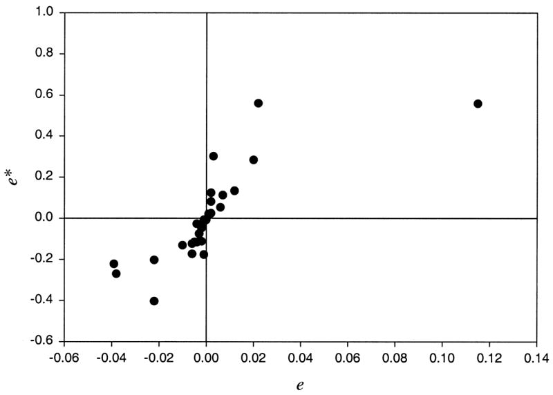
Plot of the transformed residuals $e_{ij}^{\ast }$ against the usual residuals e_ij using the empirical data.

Residuals and transformed residuals for the artificial data are shown in Table 7. They are similar in magnitude. This makes sense, because now F̃_ML = 0.029 but F̃_OLS = 0.019 as before, because the raw residuals are the same.

Table 7.

Artificial Data: Transformed Residual Matrix E* and Residual Matrix E

Variable	1	2	3	4	5	6	7	8
1.	.000	.126	−.047	−.046	−.005	.003	−.019	.022
2.	.115	.000	−.028	−.013	−.002	.014	−.013	.014
3.	−.039	−.022	.001	.027	.008	.001	.008	−.009
4.	−.038	−.010	.020	.000	−.001	−.005	.008	−.006
5.	−.004	−.001	.006	−.001	.000	.058	−.018	−.045
6.	.002	.001	.000	−.002	.022	−.005	−.009	−.008
7.	−.006	−.004	.002	.002	−.006	−.001	.001	.019
8.	.012	.007	−.005	−.003	−.022	−.002	.003	.004

Note. E* is shown above and including the diagonal, and E (from Table 3) is shown below the diagonal, for comparitive purposes.

The patterns of elements in E* and E are now very similar, and the plot of elements of E* against elements of E in Figure 2 is close to being linear.

Figure 2.

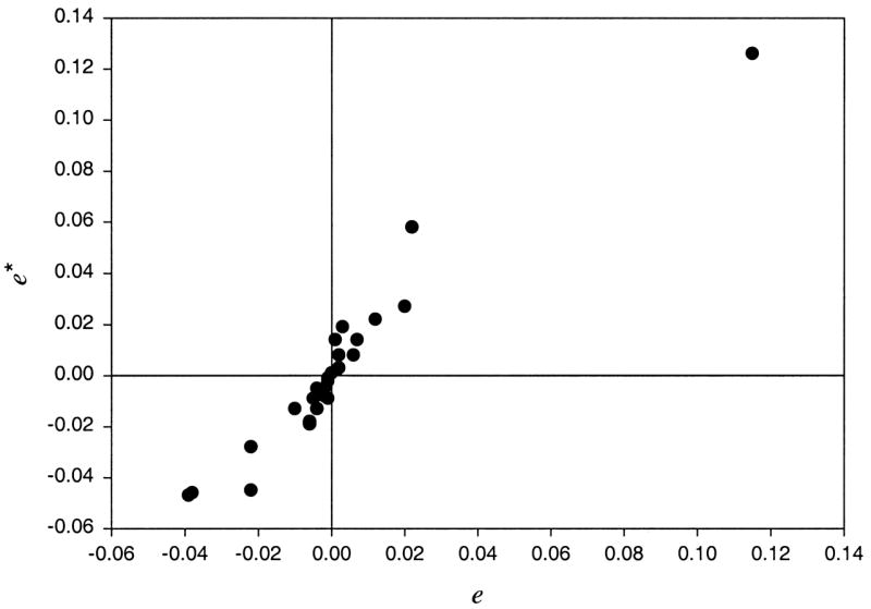
Plot of the transformed residuals $e_{ij}^{\ast }$ against the usual residuals e_ij using the artificial data.

Thus, the elements of the usual residual matrix E are entirely compatible with the OLS discrepancy function F̃_OLS in Equation 13, in that they provide all the information required to calculate it and completely determine its magnitude. The elements of E are not entirely compatible with the ML discrepancy function F̃_ML and associated generalized least squares function F̃_ML, as they do not completely determine the functions’ magnitudes. A transformed residual matrix E* has been provided in Equation 10. The elements of E* are entirely compatible with both F̂_ML and F̃_ML, as they provide all the information needed to calculate the functions, using Equations 11 and 12, and to completely determine the functions’ magnitudes. They are consequently entirely compatible with all fit measures based on either F̂_ML or F̃_ML (see Appendix A.)

Other transformed residual matrices are possible (see Appendix B), but the choice of a symmetric square root in Equation 9 ensures that the value of the element of E* associated with the element in S representing the covariance between two specific variables remains the same when the ordering of variables is changed. Equivalently, the elements of S and E* change positions in the same way when variables are reordered (see Appendix B). Because the elements of E are also associated with the corresponding elements of S, it makes sense to plot the elements of E* against corresponding elements of E to determine whether the pattern of contributions of elements of E* to F̃_ML is similar to that of elements of E to F̃_OLS. This was found to be the case to a reasonable extent with the empirical data, for which the elements of E* and E differ considerably in magnitude, and more clearly with the artificial data, for which the difference in magnitude of elements of E* and E is small.

Characteristics of the Analysis That Influence F̃_ML and F̂_ML

Inflation of F̃_ML and F̂_ML by Small Eigenvalues Σ̂

In the section titled An Illustrative Example, we showed that it is possible for the standard fit indices, which depend on E*, to give a contrary impression of goodness of fit when compared with the usual residuals (E). This incompatibility between fit indices and elements of E is most striking when elements of E* and E differ considerably in magnitude. In the present section, we examine reasons for these differences and investigate situations in which substantial incompatibilities between the usual residuals and the standard fit indices occur. Rather than compare individual elements of E* and E, it is convenient to compare the corresponding sums of squares, F̃_ML in Equation 12 and F̃_OLS in Equation 13.

To do this, we use the matrix

$$\stackrel{\sim }{\mathbf{E}}={\mathbf{U}}^{\prime }\hspace{0.17em}\hspace{0.17em}\hspace{0.17em}\mathbf{EU}.$$ (14)

Recall that matrix U contains standardized eigenvectors of Σ̂_ML. It can be shown that the elements of matrix Ẽ yield exactly the same sum of squares as the elements of E:

$${\stackrel{\sim }{F}}_{\text{OLS}}=\frac{1}{2}\sum _{i=1}^p\sum _{j=1}^p{e}_{ij}^2=\frac{1}{2}\sum _{i=1}^p\sum _{j=1}^p{\stackrel{\sim }{e}}_{ij}^2.$$ (15)

Consequently, the root mean squares of elements of E and Ẽ are the same.

A key relationship for understanding the problem at hand involves the association between the elements of Ẽ and the values of F̂_ML and F̃_ML. That relationship is given by

$${\widehat{F}}_{\text{ML}}\approx {\stackrel{\sim }{F}}_{\text{ML}}=\frac{1}{2}\sum _{i=1}^p\sum _{j=1}^p(l_i^{-1}{l}_j^{-1}){\stackrel{\sim }{e}}_{ij}^2.$$ (16)

Recall that l_i and l_j represent eigenvalues i and j of Σ̂_ML. Thus, F̃_ML is a weighted sum of squares of the elements of Σ̂ with weights $(l_i^{-1}{l}_j^{-1})$. The value of F̃_OLS, on the other hand, as shown in Equation 15, is an unweighted sum of squares of the elements of Ẽ. This distinction is critical for our understanding of why the normal-theory-based fit measures can at times contradict indications of fit given by residuals. Consider the possible situation in which the implied covariance matrix Σ̂_ML has one or more very small eigenvalues. In that situation, the inverses of those eigenvalues will be very large, resulting in the value of the quantity defined in Equation 16 becoming much larger than that in Equation 15. This observation suggests that large inverse eigenvalues of Σ̂_ML are primarily responsible for a value of F̃_ML that is much larger than that of F̃_OLS. Thus, under such conditions, fit measures based on F̃_ML or F̂_ML would indicate much poorer fit than would be indicated by the usual residuals or fit measures, such as the RMR, that are based on F̃_OLS.

Examination of results from analysis of our empirical and artificial data sets shows that the phenomenon just described does indeed account for the difference between indications of fit provided by fit measures and raw residuals. Table 8 shows eigenvalues and inverse eigenvalues of Σ̂ for the empirical and artificial data. It is clear that Σ̂ for the empirical data yields several very small eigenvalues, whereas Σ̂ for the artificial data does not. As a result, the largest inverse eigenvalues for the empirical data are many times larger than the largest inverse eigenvalues for the artificial data. This explains why in Table 5 F̃_ML and F̂_ML are many times larger than F̃_OLS for the empirical data and much closer to the same value of F̃_OLS for the artificial data. For the same reason, the elements of the transformed residual matrix E* are on average much larger for the empirical data in Table 6 than for the artificial data in Table 7.

Table 8.

Eigenvalues (l_i) and Inverse Eigenvalues $l_i^{-1}$of Σ̂

Data type and eigenvalue	1	2	3	4	5	6	7	8
Empirical
li	4.189	3.240	0.251	0.117	0.088	0.086	0.018	0.011
$l_i^{-1}$	0.239	0.309	3.978	8.576	11.390	11.655	54.945	92.593
Artificial
li	2.961	1.372	0.961	0.835	0.761	0.712	0.247	0.151
$l_i^{-1}$	0.338	0.729	1.041	1.197	1.314	1.405	4.050	6.623

The eigenvalues of Σ̂ will be close to those of S when E has small elements. Because the same near-zero E matrix applies to both data sets, the patterns of eigenvalues of Σ̂ and of S in Table 9 are similar in both cases. Small eigenvalues of Σ̂ are accompanied by small eigenvalues of S for the empirical data.

Table 9.

Eigenvalues of Σ̂ and of S

Data type and covariance matrix	1	2	3	4	5	6	7	8
Empirical
Σ̂	4.189	3.240	0.251	0.117	0.088	0.086	0.018	0.011
S	4.192	3.247	0.307	0.102	0.079	0.056	0.010	0.007
Artificial
Σ̂	2.961	1.372	0.961	0.835	0.761	0.712	0.247	0.151
S	2.959	1.378	1.028	0.786	0.742	0.712	0.244	0.151

Because all fit indices in Table 2 (and Table A1 in Appendix A), except for the RMR, are monotonic functions of either F̂_ML or F̃_ML, these indices will tend to indicate an unsatisfactory fit when some eigenvalues of Σ̂ are near zero. It is important to note that the phenomenon becomes more extreme as the number of near-zero eigenvalues increases. Each such eigenvalue contributes a large inverse eigenvalue to the quantity defined in Equation 13 and thus to further inflation of fit indices based on F̂_ML and corresponding incompatibility with raw residuals.

Table A1.

Formulas for Point Estimates of Fit Indices

Fit index	Formula	Definitionsa
Absolute fit
GFI	$\frac{p}{p+2{\stackrel{\sim }{F}}_{\text{ML}}}$	Equation 7
AGFI	$1-\frac{p(p+1)}{2d}(1-\text{GFI})$
MC	$exp\left(-\frac{1}{2}{\widehat{F}}_{\text{uHyp}}\right)$	Equations A3 and 6
Absolute misfit
RMSEA	$\sqrt{\frac{max\hspace{0.17em}({\widehat{F}}_{\text{uHyp}},0)}{d}}$	Equations A3 and 6
RMR	$\sqrt{\frac{{\stackrel{\sim }{F}}_{\text{OLS}}}{\frac{\text{1}}{\text{2}}p(p+1)}}$	Equation 13
Comparative fit
NNFI	$\frac{Q_{\text{Base}}-Q_{\text{Hyp}}}{Q_{\text{Base}}-1}$	Equation A2
NFI	$\frac{{\widehat{F}}_{\text{Base}}-{\widehat{F}}_{\text{ML}}}{{\widehat{F}}_{\text{Base}}}$	Equations A1 and 6
RNI	$\frac{{\widehat{F}}_{\text{uBase}}-{\widehat{F}}_{\text{uHyp}}}{{\widehat{F}}_{\text{uBase}}}$	Equations A3 and A4

Note. GFI = goodness-of-fit index; AGFI = adjusted goodness-of-fit index; MC = measure of centrality; RMSEA = root-mean-square error of the approximation; RMR = root-mean-square residual; NNFI = nonnormed fit index; NFI = normed fit index; RNI = relative noncentrality index.

^aThe formula in the second column involves notation defined in the specified equations.

Measurement Characteristics That Result in Striking Incompatibilities Between Residuals and Fit Measures

The preceding subsection showed that small eigenvalues of the fitted covariance matrix Σ̂ are responsible for the indications of unsatisfactory fit by all indices in Table 2 except for the RMR. This section examines practical circumstances that result in the small eigenvalues that are responsible for the indications of poor fit.

Whereas previous derivations concerning small eigenvalues of the implied covariance matrix Σ̂ did not make specific assumptions about the model, we now consider models that are of the class

$$\widehat{\mathbf{\sum }}=\widehat{\mathbf{\Lambda }}\widehat{\mathbf{\Phi }}{\widehat{\mathbf{\Lambda }}}^{\prime }+{\widehat{\mathbf{D}}}_{\psi },$$ (17)

where Λ̂ is a p × m factor matrix of rank m, and D̂_ψ is a diagonal unique factor covariance matrix with nonnegative diagonal elements. In particular, situations in which the number of common factors, m, is substantially less than the number of variables, p, are of interest. Equality constraints may be imposed on the elements of Λ̂, and the elements of the positive definite symmetric matrix Φ̂ may be functions of other parameters. Consequently, Λ̂ and D̂_ψ may be specified so as to account for the measurement model in LISREL (Jöreskog & Sörbom, 1996), and Φ̂ may be used to account for the structural model. Equation 17 therefore incorporates many LISREL models as special cases and represents a wide class of models that are used in practice.

The question under consideration is in what circumstances will models of the class in Equation 17 have some very small eigenvalues for Σ̂ and consequently yield striking incompatibilities between the residuals output by most computer programs and the fit indices output by the same computer programs. Examination of Equation 17 shows that the reproduced covariance matrix Σ̂ is the sum of two matrices. The first, Λ̂Φ̂Λ̂′, is a p × p matrix of rank m and will consequently have p − m zero eigenvalues. The second is the diagonal matrix D̂_ψ, with unique variance estimates as diagonal elements. If all these unique variance estimates were zero, Σ̂ would be equal to Λ̂Φ̂Λ̂′ and would therefore have p − m zero eigenvalues. It would be impossible to compute any of the ML fit indices because ln|Σ̂| and Σ̂⁻¹ would not exist.

Lemma C1 in Appendix C shows how the unique variance estimates in D̂_ψ strongly influence the p − m smallest eigenvalues of Σ̂ and consequently strongly influence the magnitude of the ML fit indices. It states that the p − m smallest eigenvalue of Σ̂ will lie between the largest diagonal element, ψ̂₍₁₎, and the smallest diagonal element, ψ̂_(p), of D̂_ψ. This lemma has three implications: (a) If all manifest variables have small unique variances, then marked inflation of the fit indices will occur; (b) if some manifest variables have small unique variances, marked inflation of the fit indices can occur; and (c) if none of the manifest variables have small unique variances, then marked inflation of the fit indices cannot occur.

Table 10 shows unique variance estimates for the eight variables in both the empirical and artificial data. It can be seen that in the empirical data, the last three indicators of the IFN factor have very small unique variances (≤0.022). Because inflation of fit indices was striking for the empirical data, this illustrates implication (b). For the artificial data, all unique variances exceed 0.100. Because no obvious inflation of fit indices occurred for the artificial data, this illustrates implication (c).

Table 10.

Unique Variances in Empirical and Artificial Data

Data type	NK100	NK50	NK25	NK12	IFN50	IFN25	IFN12	IFN6
Empirical	0.292	0.125	0.107	0.073	0.110	0.013	0.009	0.022
Artifical	0.971	0.860	0.798	0.710	0.782	0.183	0.124	0.286

Note. The last two numbers in the variable name refer to the first two numbers in the effector:target ratio. Thus, IFN12 represents the E:T ratio of 12.5:1 for rIFNγ. NK = natural killer; IFN = interferon.

The influence of unique variances on eigenvalues, specified in Lemma C1, may be verified by comparing unique variances in Table 10 with eigenvalues in Table 8. For the empirical data, the smallest unique variance is 0.009, and there are several eigenvalues of Σ̂ that are only slightly larger than this lower bound. As a consequence, the absolute chi-square-based fit indices in Table 2 indicate severe lack of fit. It is of interest to verify also that the smallest p − m = 6 eigenvalues are all smaller than the largest unique variance, 0.292. For the artificial data, the lower bound for eigenvalues provided by the smallest unique variance is 0.124, and the smallest eigenvalue is 0.151. The consequence is that the absolute chi-square-based fit indices in Table 2 indicate good fit for the artificial data.

A unique variance is small when both the error variance and specific variance are small so that the manifest variable not only measures with little error but also measures only characteristics that are measured by other manifest variables as well. Consequently, the fit indices can be inflated markedly only if both the specific variance and error variance of some manifest variables are small. One circumstance that can yield small specific variances and error variances would arise when highly reliable measures are used to measure the same characteristic several times. The measurements therefore are accurate in the sense of measuring the required characteristic with little error, thereby implying little specificity of the measurement process and little error of measurement.

High correlations among repeated measures of the same characteristic are symptomatic of this situation. The empirical data used in our illustration have this feature because measures of cellular immune function are quite reliable, and multiple measures using different cell concentrations are a type of repeated measure of the same characteristic. Note from Table 1 that the last three variables are very highly correlated (r_ij > .98) and appear to measure the IFN factor very accurately. Correlations between some of the NK indicators are only moderately high, and yet the chi-square-based fit indices are highly inflated. It is not essential for all correlations in the matrix to be very large for striking incompatibility between residuals and chi-square-based fit indices to be apparent.

Implications for Statistical Power

The results considered here are relevant to statistical power of tests of model fit. It is possible for a model for a population covariance matrix to be almost, but not exactly, correct and for the likelihood ratio test of exact fit to have high power. Let Σ₀ represent a population covariance matrix that fits the model under consideration closely. Suppose that θ₀ represents the vector of parameter values that minimizes F_ML[Σ₀, 𝔐(θ)] so that the fitted matrix Σ̂_ML0 = 𝔐(θ₀) is the best approximation to the population covariance matrix that satisfies the model. This yields the population discrepancy function value F̂_ML0 = F_ML(Σ₀, Σ̂_ML0). Even if the elements of the residual matrix (Σ₀ − Σ̂_ML0) are very small, it is possible for the effect size ηF_ML (Σ₀, Σ̂_ML0) to be large if some eigenvalues of Σ̂_ML0 are close to zero. This leads to high power of the likelihood ratio goodness-of-fit test, even though the model in question may fit very well, but not exactly. In other words, the probability of rejection of an almost, but not exactly, true null hypothesis will be high when some eigenvalues of Σ̂_ML0 are close to zero.

This phenomenon can be viewed as a matter of sensitivity to misspecification. The phenomena examined in this article indicate that the likelihood ratio test is differentially sensitive to misspecification of the model, depending on the eigenvalues of Σ̂_ML0. When some of those eigenvalues are near zero, then the likelihood ratio test is highly sensitive to misspecification, yielding high power. When none of those eigenvalues is close to zero, the test is less sensitive, resulting in lower power.

This observation has implications for some approaches to power analysis in structural equation modeling and factor analysis. MacCallum, Browne, and Sugawara (1996) proposed an approach to power analysis based on the RMSEA fit index. Under this approach, the investigator establishes a null hypothesis value of RMSEA, ε₀, as well as an alternative value, ε_a. Given N, α and degrees of freedom of the model, one can then calculate the power of the test of the null hypothesis assuming the specified value ε_a for the population RMSEA. As ε_a deviates further from ε₀, the calculated power increases. The developments in the current article have implications for the alternative value ε_a. For a model that yields a Σ̂_ML0. that has eigenvalues near zero, the actual RMSEA is likely to be very large, resulting in very high actual power of the test of the model. If the user of the power analysis procedure sets the specified value ε_a at some conventional value, 0.08 for example, that is considerably less than the actual RMSEA, actual power will be drastically underestimated. In a similar manner, if power analysis is used to choose sample size in advance, a larger sample size than necessary will be suggested when small eigenvalues result in an actual RMSEA that is considerably larger than the conventional value that is specified.

Extensions and Generalizations

We have examined the phenomenon of incompatibility between fit measures and residuals using a theoretical framework for analysis of covariance structures considering a particular class of models. However, our findings extend beyond the boundaries of this framework. In particular, as mentioned earlier, our findings apply in most cases to analysis of correlation structures as well as covariance structures (i.e., fitting models to correlation matrices or covariance matrices). A correlation matrix can be viewed as a rescaled covariance matrix according to

$$\mathbf{R}={\mathbf{D}}_{\text{s}}^{-1/2}\hspace{0.17em}\mathbf{S}{\mathbf{D}}_{\text{s}}^{-1/2},$$ (18)

where D_s = Diag[S]. If a model is fitted to both R and S and if the same values of F̂_ML are obtained, then the model is said to be scale invariant. For models that are scale invariant, all of the developments presented in this article hold under changes of scale of the manifest variables, such as conversion from a covariance matrix to a correlation matrix. The factor analysis model used as the hypothesized model in our illustration as well as the diagonal baseline model used for some fit indices satisfy these conditions. Most structural equation models used in practice are scale invariant. Factor analysis and structural equation models that are not scale invariant typically include specification of equality constraints or other types of constraints on parameters. For further discussion of scale invariance and the analysis of correlation structures, as opposed to covariance structures, see Cudeck (1989).

Findings presented in this article also generalize well beyond the factor analysis model used in our illustration. In an earlier section, we pointed out that the common factor covariance structure given by Σ = ΛΦΛ′ + D_ψ includes a rather broad range of structural equation models in the sense that the correlation matrix Φ for common factors can be expressed as a function of other parameters to represent a structural model for the relations among latent variables. In addition, it can be shown that our results also generalize to models that include both covariance and mean structures.⁵ Such models are commonly used for analysis of repeated measures data, for example, the latent curve models (e.g., Browne, 1993; Meredith & Tisak, 1990). In fact, the phenomenon described in this article could be especially common in such a modeling context because of the potential for low unique variances in highly correlated repeated measures of the same variable.

Summary and Conclusions

We have examined a phenomenon that occurs at times in applications of factor analysis and structural equation modeling, whereby a model that appears to fit well, as reflected by small residuals, also simultaneously yields fit indices that indicate very poor fit. It has been shown that this incompatibility can be expected when some common factors have very accurate indicators with little specificity or error. That is, marked incompatibility between residuals and chi-square-based fit indices can be expected in the presence of manifest variables with excellent measurement properties. This noticeable incompatibility is not an indication of poor research design and is not a phenomenon to be avoided. Rather it is a sign of an excellent choice of measurement instruments. One can guarantee that the incompatibility between residuals and chi-square-based fit indices is unobtrusive by choosing manifest variables with mediocre measurement properties. Obviously, this is not desirable. This phenomenon seldom occurs, however, because manifest variables in the social sciences usually have substantial errors.

It was seen that the usual correlation residuals, E, are entirely compatible with the OLS discrepancy function value, F̃_OLS, and the associated fit index, RMR. On the other hand, the transformed residuals, E*, are entirely compatible with the two alternative ML discrepancy function values, F̃_ML and F̂_ML, and all the associated ML fit indices. If one is searching for possible information explaining a large F̃_OLS, E should be examined. On the other hand, if one wishes to explain a large value of F̃_ML or F̂_ML, it would make sense to examine E*.

The occasionally noticeable incompatibility between E and F̂_ML, for example, has become apparent because most computer programs output both E and the chi-square-based fit indices. This incompatibility is, however, only a reflection of the difference between F̃_OLS and F̂_ML. These two discrepancy function values are not measures of the same thing.

For exactness, let F̃_OLS be regarded as an estimate of the corresponding quantity, F̃_OLS0, evaluated using the population covariance matrix Σ₀, and let F̂_ML be regarded as an estimate of the population quantity F̂_ML0. The population value F̃_OLS0. is a measure of misfit of the model alone and is not influenced by other characteristics of the model. As seen earlier, nF̂_ML0 is the effect size associated with the chi-square test statistic nF̂_ML. Consequently, as F̂_ML0 increases, the probability that the likelihood ratio test will correctly detect lack of fit of the model increases. If F̂_ML0 = 0, then the probability that the chi-square test will correctly detect misfit is zero. The population value F̂_ML0 is therefore best regarded as a measure of correct detectability of misfit of the model by the chi-square test. In a similar manner, the population value F̃_ML0 is a measure of misfit detectability using the alternative chi-square test statistic nF̃_ML.

Detectability of misfit depends not only on misfit but also on accuracy of measurement, as reflected in the unique variances. If the model fits exactly in the population, there is no misfit so that F̃_OLS0 is equal to zero. There is also no misfit to be detected so that F̂_ML0 and F̃_ML0 are also equal to zero, regardless of whether measurements are accurate. If F̃_OLS0 is small, but not zero, minimal misfit is indicated. If this small F̃_OLS0 is accompanied by large values of F̂_ML0 and F̃_ML0, high detectability of minimal misfit is suggested. This situation appears to apply to the empirical example. The estimates F̂_ML and F̃_ML are large, and the estimate F̃_OLS is small.

Any monotonic function of a measure of misfit is an alternative measure of misfit, and any monotonic function of a measure of misfit detectability is an alternative measure of misfit detectability. Thus, the RMR estimates a measure of misfit, and the chi-square-based fit indices estimate measures of misfit detectability. These measures of misfit detectability are functions of effect size and, although related to power, are on nonprobabilistic scales. Residuals in E may indicate reasons for misfit, but the cautions of Costner and Schoenberg (1973) should be borne in mind. If the null hypothesis in a test of fit is rejected, the rescaled residuals in E* may indicate the elements of S most responsible for this rejection.

The main advantage of chi-square-based absolute fit indices is that they have associated confidence intervals (Browne & Cudeck, 1993; Maiti & Mukherjee, 1990; Steiger, 1989) that give the information supplied by chi-square goodness-of-fit tests and also provide a range of plausible values for the index estimated. One needs to bear in mind, however, that these indices are not measuring misfit alone and that apparently large values need not in fact be unacceptable. They may be a reflection primarily of very accurate repeated measurements of the same characteristic rather than of excessive misfit.

In practice, then, when high values of chi-square-based fit measures are observed, one should not automatically conclude that the model in question is a poor one. Instead, one should carefully inspect the correlation residuals in E. If many or some of these are large, then the model may be inadequate, and the large residuals in E, or correspondingly in E*, can serve to account for the high values of misfit indices and help to identify sources of misfit. However, if all, or nearly all, of the residuals are quite small, then the phenomenon described in this article is probably operating. That is, actual model misfit is low, but that misfit is highly detectable by chi-square-based fit measures because of the presence of very low unique variances for at least some manifest variables. The investigator can verify this circumstance by examining the unique variances. In such situations, it is appropriate to conclude that the model in fact is providing a good approximation to the data but that the high indications of misfit are attributable to a high level of misfit detectability.

Appendix A

Fit Indices

The fit indices considered are functions of F̂_ML, the ML discrepancy function value for the hypothesized model (the unrestricted factor analysis model in our example) given in Equation 6 or of the corresponding generalized least squares measure F̃_ML in Equation 7. Some fit indices also use the ML discrepancy function value (see Equation 18),

$$\begin{array}{rl}{\widehat{F}}_{\text{Base}}=& -ln\mid {\mathbf{D}}_{\text{s}}^{-1/2}\hspace{0.17em}\mathbf{S}{\mathbf{D}}_{\text{s}}^{-1/2}\mid ,\\ =& -\text{ln}\mid \mathbf{R}\mid ,\end{array}$$ (A1)

for the diagonal baseline model 𝔐(σ) = D_σ.

Let d represent the degrees of freedom for the model under consideration and let d_Base = p(p − 1)/2 represent the degrees of freedom for the baseline model. Ratios of the discrepancy function values to degrees of freedom for the hypothesized model and baseline model are given by

$$Q_{\text{Hyp}}=\frac{{\widehat{F}}_{\text{ML}}}{d}$$

and

$$Q_{\text{Base}}=\frac{{\widehat{F}}_{\text{Base}}}{d_{\text{Base}}},$$ (A2)

respectively. A bias-adjusted estimate of the population ML discrepancy function value for the hypothesized model is given by

$${\widehat{F}}_{\text{u\hspace{0.17em}Hyp}}={\widehat{F}}_{\text{ML}}-\frac{d}{n},$$ (A3)

and a corresponding bias-adjusted estimate for the baseline model is given by

$${\widehat{F}}_{\text{u\hspace{0.17em}Base}}={\widehat{F}}_{\text{Base}}-\frac{d_{\text{Base}}}{n}.$$ (A4)

Formulas for the fit indices reported in Table 2 are given in Table A1. The computational formulas used for the GFI were developed independently by Maiti and Mukherjee (1990, Equation 9) and Steiger (1989, Equation 51). They are applicable to any model that is invariant under a constant scaling factor (Browne & Shapiro, 1991, Corollary 1.1). This applies to most models currently in use, including the models used in this article.

The formula given for the RMSEA in Table A1, and used for the present article, follows the approach of Browne and Cudeck (1993), in which the discrepancy function used for fitting the model is also used for the RMSEA. Steiger (1995) and Jöreskog and Sörbom (1996) compute the point estimate of the RMSEA using

$${\text{RMSEA}}_{\stackrel{\sim }{F}}=\sqrt{\frac{max({\stackrel{\sim }{F}}_{\text{uHyp}},0)}{d}},$$

where F̃_uHyp = F̃_ML − d/n, thereby replacing F̂_ML of Equation A2 by the generalized least squares fit measure F̃_ML in Equation 7. Differences between the values given by the two alternative formulas for the ML RMSEA are small when the hypothesized model fits closely. This may be seen from a comparison of F̂_ML and F̃_ML in Table 5.

Appendix B

Properties of F̂_ML, F̃_ML, and E*

Relationship Between the ML Discrepancy Function Value F̂_ML and E*

Use of Equations 6 and 10 gives

$$\begin{array}{rl}{\widehat{F}}_{\text{ML}}=& ln\mid \widehat{\mathbf{\sum }}\mid -\text{ln}\mid \mathbf{S}\mid +\text{tr}[\text{(}\mathbf{S}-\widehat{\mathbf{\sum }}){\widehat{\mathbf{\sum }}}^{-1}]\\ =& \text{tr}[{\widehat{\mathbf{\sum }}}^{-1/2}(\mathbf{S}-\widehat{\mathbf{\sum }}){\widehat{\mathbf{\sum }}}^{-1/2}]-ln\mid {\widehat{\mathbf{\sum }}}^{-1/2}\mathbf{S}{\widehat{\mathbf{\sum }}}^{-1/2}\mid \\ =& \text{tr}[\mathbf{E}\ast ]-\text{ln}\mid \mathbf{I}+\mathbf{E}\ast \mid ,\end{array}$$

which is Equation 11.

The Sum of Squared Residuals Approximation F̃_ML to F̂_ML

Use of the matrix generalization of the power series expansion of ln(1 + x) shows that the expression in Equation 11 may be expressed as the infinite series

$${\widehat{F}}_{\text{ML}}=\sum _{k=2}^{\infty }\frac{{(-1)}^k}{k}\text{tr}[\mathbf{E}{\ast }^k],$$

which converges if the eigenvalues of E* are all less than one in magnitude. Discarding terms with k > 2 yields the approximation F̂_ML ≈ F̃_ML = tr[E*²]/2. The approximation will be close if all eigenvalues of E* are sufficiently close to zero for powers greater than two to be disregarded ( $l_i^k\approx 0$, ∀i, k > 2). When this is the case, F̃_ML will be small.

Associating Elements of E* With Corresponding Elements of S

The elements of the residual matrix E may be said to be associated with corresponding elements of S in the following sense: Any reordering of the rows and columns of S, retaining symmetry, will result in exactly the same reordering of rows and columns of E. This association of elements of E with elements of S follows from the definition of E in Equation 2.

To prove that the elements of E* are associated with corresponding elements of S, we require some notation. A permutation matrix (Harville, 1997, pp. 86–88), P, is a matrix with a single 1 in each row and each column and all remaining elements equal to 0. Premultiplication of the matrix S by P reorders its rows, and postmultiplication of S by P′ reorders its columns in the same manner. Also, the symbol → represents is replaced by, ⇒ represents implies that, and ⇏ represents does not imply that.

Thus, elements of E are associated with corresponding elements of S because S → PSP′ ⇒ E → PEP′.

To prove that the elements of E* in Equation 10 are associated with corresponding elements of S if ${\widehat{\mathbf{\sum }}}_{\text{ML}}^{1/2}$ is the symmetric square root, defined in Equation 9, we use the orthogonality property of a permutation matrix, P⁻¹ = P′, and consider

$$\begin{array}{rl}\mathbf{S}\to \mathbf{PS}{\mathbf{P}}^{\prime }\Rightarrow & \widehat{\mathbf{\sum }}\to \mathbf{P}\widehat{\mathbf{\sum }}{\mathbf{P}}^{\prime }\\ \Rightarrow & \hspace{0.17em}\mathbf{U}\hspace{0.17em}\to \mathbf{PU}\\ \Rightarrow & {\widehat{\mathbf{\sum }}}_{\text{ML}}^{1/2}\to \mathbf{P}{\widehat{\mathbf{\sum }}}_{\text{ML}}^{1/2}{\mathbf{P}}^{\prime }\\ \Rightarrow & {\widehat{\mathbf{\sum }}}_{\text{ML}}^{-1/2}\to \mathbf{P}{\widehat{\mathbf{\sum }}}_{\text{ML}}^{-1/2}{\mathbf{P}}^{\prime }\\ \Rightarrow & \mathbf{E}\ast \to \mathbf{P}{\widehat{\mathbf{\sum }}}_{\text{ML}}^{-1/2}{\mathbf{P}}^{\prime }\mathbf{PE}{\mathbf{P}}^{\prime }\mathbf{P}{\widehat{\mathbf{\sum }}}_{\text{ML}}^{-1/2}{\mathbf{P}}^{\prime }=\mathbf{PE}\ast {\mathbf{P}}^{\prime }.\end{array}$$

Thus, S → PSP′ ⇒ E* → PE* P′, and we have shown that the elements of E* are associated with corresponding elements of S.

If the symmetric square root ${\widehat{\mathbf{\sum }}}_{\text{ML}}^{1/2}$ in Equation 10 is replaced by a nonsymmetric square root, ${\widehat{\mathbf{\sum }}}_{\text{ML}}^{\square 1/2}$, then the expressions for F̂_ML in Equation 11 and F̃_ML in Equation 12 will still apply, but the elements of ${\mathbf{E}}^{\square \ast }={\widehat{\mathbf{\sum }}}_{\text{ML}}^{\square -1/2}\hspace{0.17em}\mathbf{E}{\widehat{\mathbf{\sum }}}_{\text{ML}}^{\square -1/2}\prime$ can no longer be associated with corresponding elements of S. This follows because $\mathbf{S}\to \mathbf{PS}{\mathbf{P}}^{\prime }\nRightarrow {\widehat{\mathbf{\sum }}}_{\text{ML}}^{\square -1/2}\to \mathbf{P}{\widehat{\mathbf{\sum }}}_{\text{ML}}^{\square -1/2}\hspace{0.17em}{\mathbf{P}}^{\prime }$, so that S → PSP′ ⇏ E^□* PE^□* P′.

It is instructive to consider a particular nonsymmetric square root of Σ̂_ML, namely, the principal components square root ${\widehat{\mathbf{\sum }}}_{\mathit{ML}}^{\square 1/2}=\mathbf{U}\hspace{0.17em}{\widehat{\mathbf{D}}}_l^{1/2}$. Then the transformed residual matrix is ${\mathbf{E}}^{\square \ast }={\widehat{\mathbf{D}}}_l^{-\text{1}/\text{2}}\hspace{0.17em}{\mathbf{U}}^{\prime }\hspace{0.17em}\mathbf{EU}\hspace{0.17em}{\widehat{\mathbf{D}}}_l^{-1/2}$ and does not change when variables are reordered. Consequently, reordering of variables does not reorder the rows and columns of E^□* in a manner that corresponds to the reordering of rows and columns of S. Any attempt to associate elements of E^□* with those of S would therefore be arbitrary and would become invalid as soon as the ordering of variables is changed.

When a Cholesky (triangular) square root is used, the values of elements of the matrix square root change when the variables are reordered. Consequently, the values of elements of the transformed residual matrix also change with any reordering of variables.

Appendix C

Relationships Between Unique Variances and Eigenvalues

This appendix states a lemma that is helpful when investigating the relationship between accuracy of measurement and closeness of the smallest eigenvalues of a reproduced covariance matrix Σ to zero.

Definitions

Suppose that Φ is a m × m nonnegative definite matrix, Λ is a p × m matrix of rank m, and D_ψ is a p × p nonnegative definite diagonal matrix. Let the eigenvalues, λ_i, i = 1, …, p, of Σ be arranged in decreasing order of magnitude. Elements of D_ψ are not arranged in descending order of magnitude. The largest will be represented by ψ₍₁₎ and the smallest by ψ_(p).

Lemma C1

The smallest p − m eigenvalues of Σ are contained in the interval between the largest and the smallest unique variances:

$${\psi }_{\text{(1)}}\ge {\lambda }_{m+1}\ge {\lambda }_{m+2}\ge \dots \ge {\lambda }_p\ge {\psi }_{\text{(}p\text{)}}.$$

Proof

Let λ_i (W) represent the ith eigenvalue of a symmetric matrix W, arranged in descending order of magnitude. Lemma 1 of Ostrowski (1959) shows that

$${\mathbf{\lambda }}_i(\mathbf{\sum })={\mathbf{\lambda }}_i(\mathbf{\Lambda }\mathbf{\Phi }{\mathbf{\Lambda }}^{\prime })+{\mathbf{\epsilon }}_i,$$

where λ₁(D_ψ) ≥ ε_i ≥ λ_p(D_ψ), i = 1,…, p. Because the smallest p − m eigenvalues of ΛΦΛ′ are zero, the result follows.

References

- Andersen BL, Farrar WB, Golden-Kreutz D, Katz LA, MacCallum RC, Courtney ME, Glaser R. Stress and immune response after surgical treatment for regional breast cancer. Journal of the National Cancer Institute. 1998;90:30–36. doi: 10.1093/jnci/90.1.30. [DOI] [PMC free article] [PubMed] [Google Scholar]
- Andersen BL, Kiecolt-Glaser JK, Glaser R. A biobehavioral model of cancer stress and disease course. American Psychologist. 1994;49:389–404. doi: 10.1037//0003-066x.49.5.389. [DOI] [PMC free article] [PubMed] [Google Scholar]
- Bentler PM. Comparative fit indices in structural models. Psychological Bulletin. 1990;107:238–246. doi: 10.1037/0033-2909.107.2.238. [DOI] [PubMed] [Google Scholar]
- Bentler PM, Bonnett DG. Significance tests and goodness of fit in the analysis of covariance structures. Psychological Bulletin. 1980;88:588–600. [Google Scholar]
- Bollen KA. Structural equations with latent variables. New York: Wiley; 1989. [Google Scholar]
- Browne MW. Structured latent curve models. In: Cuadras CM, Rao CR, editors. Multivariate analysis: Future directions 2. Amsterdam: North-Holland; 1993. pp. 171–198. [Google Scholar]
- Browne MW, Cudeck R. Alternative ways of assessing model fit. In: Bollen KA, Long JS, editors. Testing structural equation models. Newbury Park, CA: Sage; 1993. pp. 136–161. [Google Scholar]
- Browne MW, Shapiro A. Invariance of covariance structures under groups of transformations. Metrika. 1991;38:345–355. [Google Scholar]
- Costner HL, Schoenberg RJ. Diagnosing indicator ills in multiple indicator models. In: Goldberger AS, Duncan OD, editors. Structural equation models in the social sciences. New York: Seminar Press; 1973. pp. 167–199. [Google Scholar]
- Cudeck R. Analysis of correlation matrices using covariance structure models. Psychological Bulletin. 1989;105:317–327. [Google Scholar]
- Harville DA. Matrix algebra from a statistician’s perspective. New York: Springer-Verlag; 1997. [Google Scholar]
- Hu L, Bentler PM. Fit indices in covariance structure modeling: Sensitivity to underparameterized model misspecification. Psychological Methods. 1998;3:424–453. [Google Scholar]
- Jöreskog KG, Sörbom D. LISREL VI: User’s guide. 3. Mooresville, IN: Scientific Software, Inc; 1984. [Computer software manual] [Google Scholar]
- Jöreskog KG, Sörbom D. LISREL 8: User’s reference guide [Computer software manual] Chicago: Scientific Software, Inc; 1996. [Google Scholar]
- MacCallum RC, Browne MW, Sugawara HM. Power analysis and determination of sample size for covariance structure modeling. Psychological Methods. 1996;1:130–149. [Google Scholar]
- Maiti SS, Mukherjee BN. A note on distributional properties of the Jöreskog–Sörbom fit indices. Psychometrika. 1990;55:721–726. [Google Scholar]
- McDonald RP. An index of goodness of fit based on noncentrality. Journal of Classification. 1989;6:97–103. [Google Scholar]
- McDonald RP, Marsh H. Choosing a multivariate model: Noncentrality and goodness of fit. Psychological Bulletin. 1990;107:247–255. [Google Scholar]
- Meredith W, Tisak J. Latent curve analysis. Psychometrika. 1990;55:107–122. [Google Scholar]
- Nelder JA, Mead R. A simplex method for function minimization. Computer Journal. 1965;7:308–313. [Google Scholar]
- Ostrowski AM. A quantitative formulation of Sylvester’s Law of Inertia. Proceedings of the National Academy of Sciences, USA. 1959;45:740–744. doi: 10.1073/pnas.45.5.740. [DOI] [PMC free article] [PubMed] [Google Scholar]
- Steiger JH. EzPATH: A supplementary module for SYSTAT and SYGRAPH. [Computer software manual] Evanston, IL: SYSTAT; 1989. [Google Scholar]
- Steiger JH. Statistical/W (Version 5) [Computer software and manual] Tulsa, OK: StatSoft; 1995. Structural equation modeling (SEPATH) pp. 3539–3688. [Google Scholar]
- Steiger JH. Point estimation, hypothesis testing and interval estimation using the RMSEA: Some comments and a reply to Hayduk and Glaser. Structural Equation Modeling. 2000;7:149–162. [Google Scholar]
- Steiger JH, Lind JM. Statistically based tests for the number of common factors; Paper presented at the annual meeting of the Psychometric Society; Iowa City, IA. 1980. Jun, [Google Scholar]
- Tucker LR, Lewis C. A reliability coefficient for maximum likelihood factor analysis. Psychometrika. 1973;38:1–10. [Google Scholar]