

Abstract
A new model for aspects of the control of respiration in mammals has been developed. The model integrates a reduced representation of the brainstem respiratory neural controller together with peripheral gas exchange and transport mechanisms. The neural controller consists of two components. One component represents the inspiratory oscillator in the pre-Bötzinger complex (pre-BötC) incorporating bio-physical mechanisms for rhythm generation. The other component represents the ventral respiratory group (VRG), which is driven by the pre-BötC for generation of inspiratory (pre)motor output. The neural model was coupled to simplified models of the lungs incorporating oxygen and carbon dioxide transport. The simplified representation of the brainstem neural circuitry has regulation of both frequency and amplitude of respiration and is done in response to partial pressures of oxygen and carbon dioxide in the blood using proportional (P) and proportional plus integral (PI) controllers. We have studied the coupled system under open and closed loop control. We show that two breathing regimes can exist in the model. In one regime an increase in the inspiratory frequency is accompanied by an increase in amplitude. In the second regime an increase in frequency is accompanied by a decrease in amplitude. The dynamic response of the model to changes in the concentration of inspired O2 or inspired CO2 was compared qualitatively with experimental data reported in the physiological literature. We show that the dynamic response with a PI-controller fits the experimental data better but suggests that when high levels of CO2 are inspired the respiratory system cannot reach steady state. Our model also predicts that there could be two possible mechanisms for apnea appearance when 100% O2 is inspired following a period of 5% inspired O2. This paper represents a novel attempt to link neural control and gas transport mechanisms, highlights important issues in amplitude and frequency control and sets the stage for more complete neurophysiological control models.
Keywords: Neural control, Respiration, Gas exchange, Apnea
1 Introduction
The respiratory system in mammals consists of neural elements in the brain and peripheral gas exchange and transport apparatus. Breathing movements are produced by neural networks in the brainstem that generate rhythmic patterns of neural activity that drive the respiratory muscles, providing air flow into and out of the lungs for gas exchange, transport, and homeostatic regulation of blood oxygen and carbon dioxide. Regulation of oxygen and carbon dioxide is accomplished by chemosensors outside and within the central nervous system that feedback signals to the brainstem networks for control of respiratory movements appropriate for lung ventilation. Understanding the integrated operation of this system remains a major problem in the respiratory biology and neuroscience fields.
Several mathematical models have been developed in the past to study the integrated operation of the respiratory system (see Batzel et al., 2006; Khoo and Yamashiro, 1989; Topor et al., 2004, for a comprehensive review). Many models represent the lungs as a constant-volume compartment with a continuous unidirectional fow of air. The controlled variable in these models is the minute ventilation (i.e., the volume of air inhaled per minute) while the controller (representing the central nervous system) is a "black box" model which provides a mathematical relationship between blood partial pressures of O2 and CO2 and minute ventilation (see for example Batzel and Tran, 2000; Carley and Shannon, 1988; Fowler and Kalamangalam, 2002; Grodins et al., 1967; Topor et al., 2004; Ursino et al., 2001a,b). Other, so called "breathing" models, have taken the ventilation or the ventilation drive as a sinusoidal function of time where the instantaneous amplitude and frequency depend on the blood partial pressures of O2 and CO2 (see for example Khoo and Yamashiro, 1989; Lu et al., 2002; Saunders, 1980). There have been a few attempts to couple neural activity in the brainstem to lung models. Eldridge (1996) has used the Fitzhugh-Van der Pol-Bonhoeffer oscillator to represent the neural controller and coupled it to mass balance equations for O2 and CO2 exchange (taking minute ventilation into account). Rybak et al. (2004) coupled a detailed description of the respiratory network to a simplified model of the lungs that provided mechanosensory feedback related to the amplitude of the neural drive (representing feedback from pulmonary stretch receptors indicating lung volume) but ignored gas exchange and chemical feedback. Most recently, Longobardo et al. (2005) have adapted models of respiratory pattern generators into a neurochemical feedback control model of ventilation. The tidal volume and frequency were both obtained from the respiratory pattern generator output by scaling the activity pattern and were then used to estimate the minute ventilation.
In this paper we couple together, for the first time, essential features of the dynamical operation of brainstem neural circuits with peripheral lung gas exchange apparatus and transport where ventilation is not averaged over time. While our model can be called a "breathing" model, the ventilation drive is not a sinusoidal function but a non-symmetric signal representing the output of the neural system. The example of an integrated model we present in this paper incorporates recent advances in modeling the dynamical activity patterns of respiratory networks on the one hand (Butera et al., 1999a,b; Rybak et al., 2004; Smith et al., 2000, 2007), and new mathematical models for gas exchange and transport on the other hand (Ben-Tal, 2006), setting the stage for development of unified respiratory system models.
The brainstem respiratory networks comprise of a central pattern generator (CPG) that produces the neural oscillation underlying the breathing rhythm and controls temporal patterns of neural population activity during inspiration and expiration (Feldman and Smith, 1995; Richter, 1996). The most elaborate CPG models incorporate neuronal biophysical properties that have been proposed to account for the rhythmic activity patterns of interacting neuronal populations within distributed networks (Rybak et al., 1997a,b, 2004; Smith et al., 2000, 2007). Respiratory rhythm generation in such models emerges from inhibitory and excitatory interactions and intrinsic cell biophysical properties operating in part at the level of the pre-Bötzinger complex (pre-BötC) (Smith et al., 1991) – the circuit component generating rhythmic excitatory drive in the network during inspiration (Smith et al., 2000). The operation of these complex models with regard to control of frequency and amplitude of inspiratory activity that regulates ventilation is poorly understood however. Independent control of inspiratory frequency and amplitude is a basic operational feature of the respiratory CPG critical for regulation of ventilation by chemosensory feedback signals (e.g. Feldman, 1986; Feldman et al., 1988). Here we developed a simplified representation of the CPG that focuses primarily on the pre-BötC, including biophysical processes involved in control of inspiratory frequency. Our model also represents downstream neural elements of the ventral respiratory group (VRG) that are essential for separate control of amplitude of the excitatory inspiratory drive to the diaphragm. This approach allows us to explicitly consider inspiratory frequency and amplitude control and circumvents the limitation on the maximum minute ventilation encountered in other recent attempts to couple simplified models of the CPG with neurochemical feedback control (Longobardo et al., 2005).
In this work we have adopted the model of Ben-Tal (2006) with modifications that allowed us to couple the neural control model to simplified models of the lungs incorporating oxygen and carbon dioxide transport. One problem in linking the neural controller to gas transport mechanisms and feedback signals is that the dynamics of the control signals related to the controlled variables (oxygen and carbon dioxide) as well as how these signals operate at level of the neural system are poorly understood. We therefore evaluated several standard feedback mechanisms that are well known in control theory. The dynamic responses of the model to changes in the concentration of inspired oxygen or carbon dioxide were compared qualitatively with experimental data, and we found that the model mimics and provides possible explanations for a number of features of these experiments.
The model we present in this paper does not include some of the features that other models have taken into account. For example, our model does not include delay in the circulatory system and does not take into account mechanoreceptor feedback signals from the pulmonary stretch receptors. These features can be added to the model but we left them out for the sake of simplicity. Other features such as gas exchange at the tissue level are taken into account indirectly in our model. We have chosen to focus our attention in this paper on coupling between the neural control system and a "breathing" model and illustrate the benefits of such approach. The parameters and variables that appear frequently in the paper are listed in Appendix A. Most parameters have physiologically realistic values that have been published in the literature but we have not attempted to fit the values of the parameters to a specific experiment. Instead we look for qualitative differences in the outcome of different model configurations for a range of experiments.
2 Reduced neural control model
Our neural model incorporates separate mechanisms for oscillatory activity generation and generation of inspiratory activity pattern in a configuration that allows for independent control of inspiratory frequency and the amplitude of inspiratory neural drive to the lung diaphragm (Fig. 1).
Fig. 1.
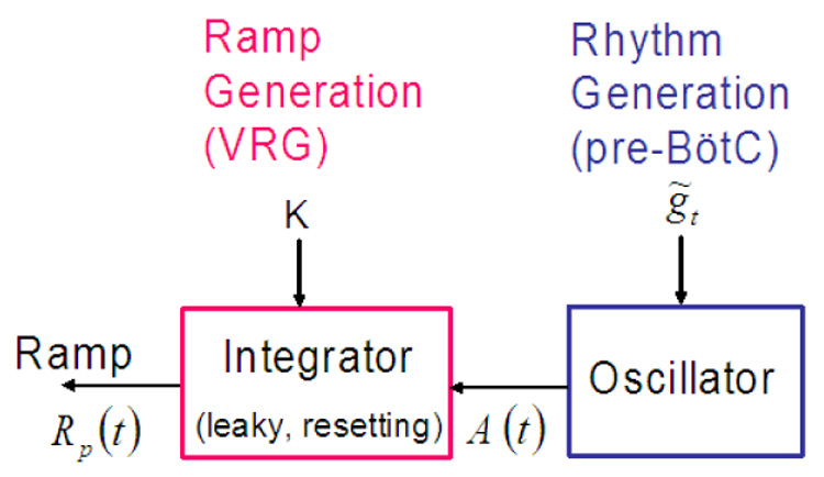
Reduced neural control model.
The model consists of two interacting components: an oscillator responsible for rhythm generation and an inspiratory pattern generator that is driven by the oscillator and transforms the drive in a ramp pattern of neural activity. We represent the transformation of the drive from the pre-BötC oscillator into a ramping neural signal as a leaky integration process. This ramping waveform is characteristic of the neural elements in the ventral respiratory group (VRG) of the medulla that drive the diaphragm and lung ventilation. The ramp signal is the control model output and serves as an input signal to the diaphragm. Frequency and amplitude are controlled by the two parameters K and . Next we describe each of the control model components in detail and show how frequency and amplitude can be controlled.
2.1 Rhythm generation (pre-BötC)
We denote the level of activity of the pre-BötC population by A. A is a measure of the average spike rate in the population at a given time unit. We assume that 0 ≤ A ≤ 1. When A = 0 all the neurons in the population are inactive while A = 1 represents a fully active and synchronized population which fires at the highest possible rate. The dynamics of the pre-BötC population activity can then be described by the following general form:
| (1) |
where α (1 − A) is the rate by which A becomes active, βA is the rate by which A becomes inactive and γ is an external drive (could be inhibitory or excitatory). α, β and γ are functions of the excitatory and inhibitory drives. Note that "activity" is strongly related to voltage since a neuron is "active" once the voltage across its membrane is above a certain threshold. Thus the population activity, A, can be related to the average voltage, υ, by the linear transformation A = ãυ + b̃ (see also Tabak and Rinzel, 2005). We use this transformation to show that the control parameter used in the activity model can be related to the external drive in the voltage-based model and to justify the choice of parameter values (see Appendix C).
Rhythm generation in the actual neural system is complex and involves interactions between several populations of neurons. For simplicity, we do not consider here complex network interactions such as inhibitory synaptic mechanisms that arise during expiration and operate at the level of the pre-BötC. It has been shown both computationally and experimentally that without the network interactions, persistent sodium current plays a major role in the control of the respiratory period (Butera et al., 1999a; Del Negro et al., 2001, 2002; Smith et al., 2007). The coefficients in Eq. (1) therefore take the form: are parameters (whose physiological meaning are explained in Appendix C), hp is a variable representing the inactivation gating of persistent sodium current and is the activation gating of persistent sodium current in steady state (we assume here that the activation gating is a fast process). is given by:
| (2) |
where are parameters. The dynamics of hp is described by the equation:
| (3) |
where
| (4) |
are parameters. The parameter values are given in Appendix A.
Fig. 2 shows the model output which mimics the behaviour of the pre-BötC as seen experimentally (e.g. Del Negro et al., 2001; Smith et al., 2007). Note that when hp reaches its maximum A starts to decay. Fig. 3 shows how the parameter controls the frequency. Changes in represent different levels of external drive to the pre-BötC and we therefore chose it as our control parameter. Note that there are three states in Fig. 3: 1) low level activity equilibrium which is equivalent to a silence state in the neural system; 2) oscillation which is equivalent to rhythmic bursting in the neural system and 3) high level activity equilibrium which is equivalent to the beating (continuous spiking, tonic) activity state in the neural system. When the pre-BötC is in an oscillatory bursting state an increase in increases the frequency. Note that the level of activity for the low frequency (for example when gn = 8) is higher than the level of activity for the high frequency (for example when gn = 18). This indicates that the spike frequency in the neural population is higher at low bursting frequency and is consistent with experimental observations (Del Negro et al., 2001).
Fig. 2.
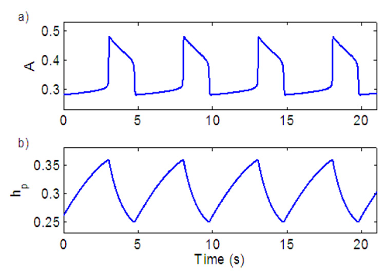
Model output of the neural oscillator (pre-BötC). a) Population activity. b) Inactivation gating of persistent sodium.
Fig. 3.
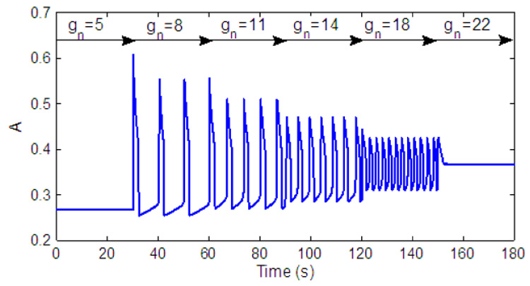
Output of the pre-BötC for different values of gn (nominal value of ).
2.2 Ramp generation (VRG)
We assume that ramp generation can be described conceptually as a leaky integration. In the neurological system the VRG "integrator" is released from inhibition just at the step onset of the pre-BötC activity (the signal A in our model). We mimic this by introducing a threshold for A (Tr1) above which integration starts. A crucial factor for maintaining the ramp evolution in the neural system is a steady external excitatory drive to the ramp generator. Neurophysiologically such an excitatory drive is presumed to come from extrinsic groups of neurons involved in sensing CO2 and O2. This continuous baseline excitation is represented in our model by the constant K which is added to the integrated signal and therefore influences the amplitude of the ramp signal. Amplitude control in the real system with lungs intact also involves mechanoreceptor inputs that operate as a resetting mechanism (in part) at the level of VRG (i.e. the "inspiratory off-switch"). Furthermore, the ramp generator is terminated (reset) by post-inspiratory inhibitory neurons that are released from inhibition as inspiratory activity of the pre-BötC declines. We mimic this in our model by resetting the ramp signal to zero once the signal A is below a given threshold (Tr2). Conceptually the threshold termination mechanism that we use can be viewed as the combined effect of the decline of pre-BötC excitatory drive and termination related to the amplitude of VRG integrator activity. It would be a trivial extension of our integrator model to assign a separate threshold related specifically to the amplitude of VRG activity. When A is in a "beating" state (i.e., in a high level activity equilibrium) the leaky integrator will eventually reach a saturation point. We introduce another threshold (Tr3) that could be set at a lower saturation point. This could represent an external signal that stops the integration but not reset it. Mathematically, we calculate the ramp signal, Rp(t), as follows:
| (5) |
where Ip = Il * ((A(t − Δt) + A(t)) * Δt/2 + Rp (t − Δt)) is the calculated integral (using the trapezoidal rule of integration), Il is a constant (Il < 1 for a leaky integrator), Δt is the time step in the numerical solution and ε is a positive small number. Note that we added another threshold (Tr4) to ensure that if K is small enough integration will not occur (Rp(t) will be reset to the value of K at each time step). Also note that when Rp(t − Δt) > Tr3 we add another condition to ensure that A is in equilibrium. In our simulations Tr1 = Tr2 = 0.35, Tr4 = 0.001 and ε = 1 × 10⁻⁵. For values of Il see Fig. 5. Tr3 can be chosen arbitrarily.We have used numerical integration for the operation of the integrator. One could also explicitly formulate a leaky integrator model derived from equations for the activity or firing rate of a recurrently connected excitatory neural population receiving inputs from other populations (Seung, 2003).
Fig. 5.
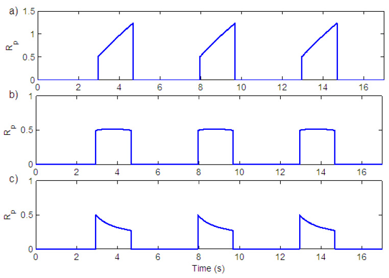
Effect of leak in the integrator on the shape of the ramp. a) Il = 0.99999 b) Il = 0.99915 c) Il = 0.9984.
Fig. 4 shows ramp generation for the three states that exist in the neural system. The silent state is an equilibrium with a low level of activity in the rhythm generator (Fig. 4, b.3). Since the output of the oscillator (A) is below a threshold, integration in the ramp generator have not started and the ramp signal is in equilibrium at zero (Fig. 4, a.3). The bursting state (represented by a periodic solution) is seen in Fig. 4, a.2 and b.2. Once the oscillator output is above a threshold, K is added to the ramp signal and integration starts. Once the oscillator output is below a threshold the ramp is reset back to zero. The beating state is represented by an equilibrium with a high level of activity in the rhythm generator (Fig. 4, b.1). Because the value of A (the oscillator output) is now above the threshold the signal will be integrated continuously until it reaches a saturation point (Fig. 4, a.1).
Fig. 4.
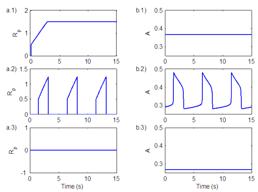
Ramp generation for the three states that exist in the neural system. a) Ramp output. b) Oscillator (pre-BötC) output. 1) Beating (tonic) state. 2) Bursting (breathing) state. 3) Silence state.
The amount of leak in the integrator (Il) will affect the shape of the ramp. Fig. 5 shows ramp signals for different values of Il. In graph a) Il = 0.99999 in b) Il = 0.99915 and in c) Il = 0.9984. All of these different shapes have been seen experimentally (Smith et al., 2007). Graph a) corresponds to normal breathing and graph c) corresponds to gasping, usually seen under conditions of severe hypoxia. In this case the output of the integrator follows the wave form of the pre-BötC activity (Paton et al., 2006).
2.3 Amplitude control in the neural model
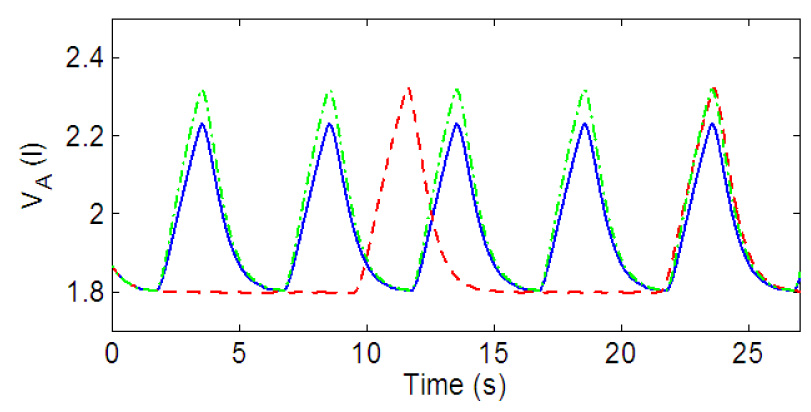
The amplitude of breathing can be controlled by the three parameters , K and Il. When is varied the frequency of breathing is changed. An increase in frequency results in a decrease in amplitude due to the decrease in inspiration time as seen in Fig. 6 a). By varying K the amplitude of breathing can be changed without changing the frequency (Fig. 6 b)). Amplitude could also be controlled by changing the amount of leak (Il) in the integrator (Fig. 6 c)). These three mechanisms to vary the amplitude have been documented experimentally (Feldman, 1986; Feldman et al., 1988). The case represented by Fig. 6 b (varying K) is typical of the amplitude response seen with changes of CO2 (e.g. Feldman, 1986). We have therefore adapted this as a primary mechanism of amplitude control in our model.
Fig. 6.
Amplitude control in the neural model. a) Variation in gn (change in the duration of inspiration). Solid (blue) line - gn = 17, (Kn = 0.5), Dashed (red) line - gn = 7, (Kn = 0.5) b) Variation in Kn. Solid (blue) line - Kn = 0.2, (gn = 7), Dashed (red) line - Kn = 0.5, (gn = 7). c) Variation in the amount of leak in the integrator. Solid (blue) line - Il = 0.9995, Dashed (red) line - Il = 0.99999. Kn = 0.5, gn = 7 in both graphs.
3 Coupling the neural model with peripheral gas exchange model
The neural control model was coupled to simplified models of the lungs incorporating oxygen and carbon dioxide transport. A schematic description of the integrated model is shown in Fig. 7. Each of the model compartments is described below.
Fig. 7.
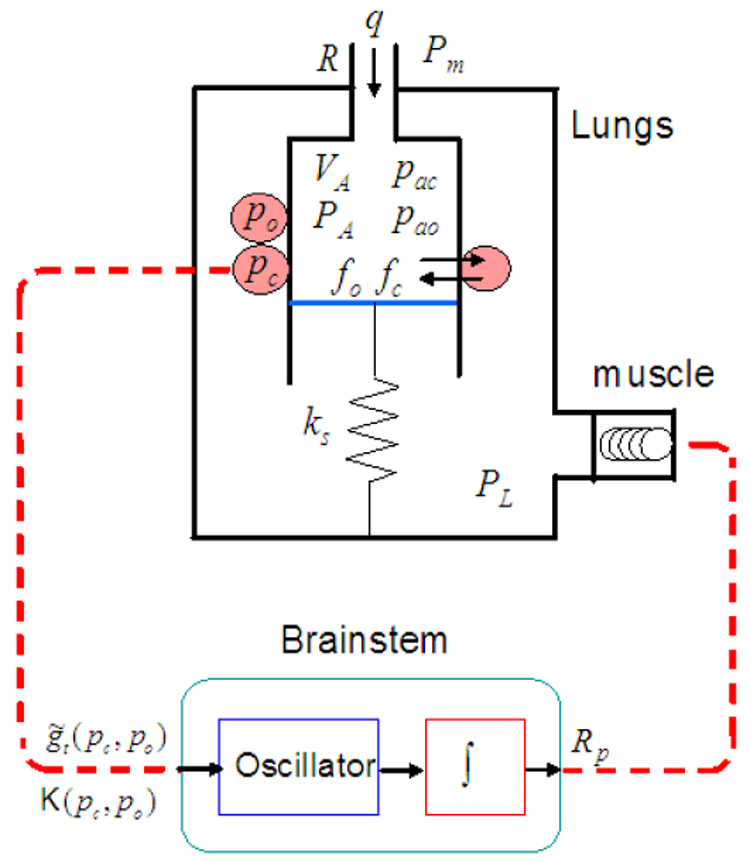
The integrated model. VA - total lung volume, PA - average alveolar pressure, Pm - mouth pressure, PL - pleural pressure, q - air flow, R - overall resistance of the conducting airways, ks - spring constant (note that spring compression represents lung expansion and that the lung elastance, E, is equivalent to ks/s2 where s is the area of the moving plate). fo and fc are the alveolar concentrations of oxygen and carbon dioxide respectively. pao and pac are the alveolar partial pressures of oxygen and carbon dioxide, respectively. po and pc are the blood partial pressures of oxygen and carbon dioxide, respectively. Rp is the ramp signal from the brainstem that activates the muscle. and K are control variables in the brain stem compartment that are functions of po and pc.
3.1 Muscle compartment
The electrical signal from the neural controller is transmitted to spinal motor neurons to produce contraction of respiratory muscles. The level of intensity of muscle contraction is controlled by two main mechanisms (Guyton and Hall, 2000): 1) change in the frequency of contraction (called frequency summation that can lead to tetanization) and 2) change in the number of motor units recruited. Here we ignore the frequency summation and assume that recruitment of motor units is the main mechanism for the control of muscle contraction. We assume that the force generator at the level of muscle is following the wave form of phrenic nerve activity (the ramp signal in our model) and that this is the essential representation for muscle force production and pleural pressure wave form generation.
We model the muscle as a spring, excited by an external force. The muscle displacement xm is modelled by
| (6) |
The pleural pressure, PL, is modelled by
| (7) |
where Pm is the mouth pressure and PL0 is the difference that normally exists between atmospheric and pleural pressures (Comroe, 1977). Fig. 8 shows the ramp signal and the resulting pleural pressure. The shape of the pleural pressure signal is consistent with measurements of pleural pressure (e.g. D’angelo et al., 1974).
Fig. 8.
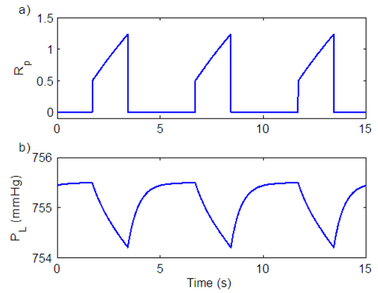
Pleural pressure generation. a) Ramp signal. b) Pleural pressure signal.
3.2 Lung compartment
The lung is modeled by a single container which has a moving plate attached to a spring (see Fig. 7). Gas exchange and gas transport are modeled by a "conveyor" model shown in Fig. 9. It is assumed that the volume of the capillaries is the same as the heart stroke volume and that the transit time of blood through the lung is the same as the time interval between heart beats. The mathematical equations for the lung model have been developed in (Ben-Tal, 2006) but some modifications have been made in the integrated model. For convenience the entire equations are given here and the modifications are pointed out.
| (8) |
where PA is the alveoli total pressure (averaged over all the alveoli in the different regions of the lungs). fo and fc are the concentrations of oxygen and carbon dioxide, respectively. po and pc are the blood partial pressures of oxygen and carbon dioxide, respectively. is the concentration of bicarbonate in the blood. Pm is the mouth pressure (assumed to be constant), PL is the pleural pressure and E is the lung elastance. Do and Dc are the diffusion capacities (transfer factors) of oxygen and carbon dioxide, respectively, pao = fo (PA − pw) and pac = fc (PA − pw) are the alveolar partial pressures of oxygen and carbon dioxide, respectively, where pw is the vapor pressure of water at 37°C. QA = q + Dc (pc − pac) + Do (po − pao) is the net flux of gas into the alveoli where is the air flow and R is the airways resistance to flow. qi is the inspired air flow (note that since foi = fo and fci = fc on expiration, qi ≡ q, see Eq. (9)). f̃(po) is the saturation function of hemoglobin (see Eq. (12)), l2 is the hydration reaction rate, r2 is the dehydration reaction rate, and h = [H+] is the concentration of hydrogen ions (which is constant in this model). Vc is the capillary volume, σ is the solubility of oxygen, σc is the solubility of carbon dioxide, Th is the concentration of the hemoglobin molecules in the blood and δ is a free parameter in the model representing the effect of the enzyme carbonic anhydrase on the chemical reaction. is the total volume of the lungs where E is the lung elastance and V0 is the volume of the lungs when it is unloaded (Vo = 0 in our model). foi and fci are the inspired concentrations of oxygen and carbon dioxide respectively and are calculated by the following formula
| (9) |
VD is the lung dead space volume, fod is the concentration of oxygen in the lung dead space (calculated as the lung concentration of oxygen at the end of expiration) and fom is the concentration of oxygen in the mouth. Vi is the inspired volume of the lungs and is calculated by integrating the airflow during inspiration using the trapezoidal rule of integration as follows.
| (10) |
Equation (9) differs from the original model in Ben-Tal (2006) where Vi is replaced by VT, the tidal volume, and when VT > VD. In Ben-Tal (2006), VT is a parameter and the pleural pressure, PL, is a given function of VT. In the integrated model VT cannot be estimated a priori and needs to be calculated. At the end of inspiration Vi = VT. This different calculation of foi does not influence the output of the model significantly.
Fig. 9.
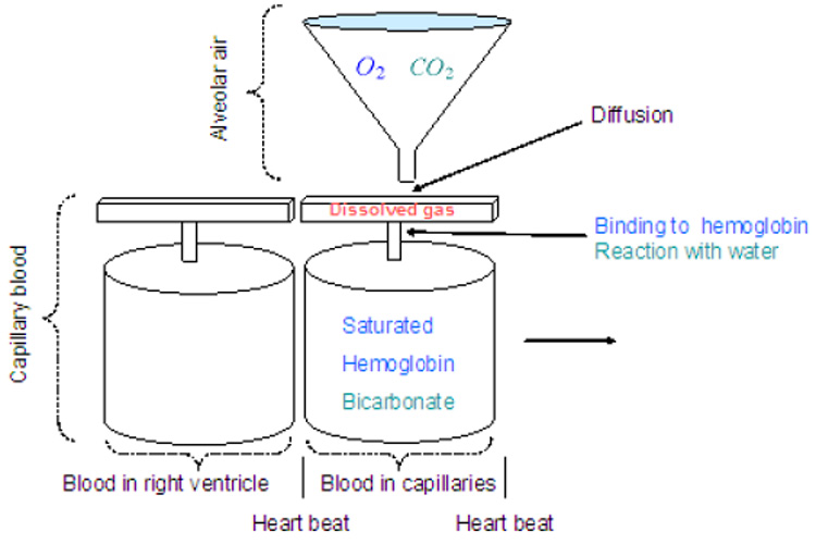
A model for gas exchange and gas transport (after Ben-Tal, 2006).
The inspired concentration of carbon dioxide is calculated as in Eq. (9) with foi, fod and fom replaced by fci, fcd and fcm, respectively.
The moving "conveyor" is simulated by re-initializing the values of pc, po and z every heart beat (see Ben-Tal, 2006, for more details). The values of pc and po at the end of each inter-beat interval (i.e. just before they are re-initialized) represent the blood partial pressures at the end of the capillaries. These values are stored as pce and poe and are updated every heart beat.
One difference between the lung model here and the lung model in Ben-Tal (2006) is that in the previous model, the pleural pressure has been taken as sinusoidal in most of the numerical simulations and hence the signal was symmetric with inspiration time equals the expiration time. Here the pleural pressure is the output from the neural system model. The signal is not symmetric and the inspiration time is about a third of the respiration period (similar to the physiological system).
3.3 Feedback modelling
Recall that and K are control parameters that represent inputs to the neural control component. In an open loop control and K have set values. In a closed loop control they are functions of the partial pressures of oxygen and carbon dioxide. The exact feedback mechanism in the physiological system is not known yet. We therefore use some standard feedback functions that are well known in control theory (see for example Parr, 1996). We study different feedback mechanisms and show that they lead to qualitative differences in the results. To simplify the mathematical expressions the following "errors" are defined:
| (11) |
where Erc is the "error" in the level of carbon dioxide and Ero is the "error" in the level of oxygen. pce and poe are the partial pressures of carbon dioxide and oxygen at the end of the capillary, respectively. pcr and por are reference values (in our simulations pcr = 40 mmHg and por = 104 mmHg, the average values of pce and poe under normal conditions). f̃ is the saturation function of hemoglobin given by (Ben-Tal, 2006; Monod et al., 1965):
| (12) |
where L, KT and KR are parameters.
Note that in all the simulations shown in this paper pce = pce (t) and poe = poe (t), that is, delays in the circulatory system are not taken into account. Delays can be included by taking pce = pce (t − Τ1) and poe = poe (t − Τ2) where Τ1 and Τ2 are the time delays in the circulation; Τ1 could represent the travel time to the chemosensitive areas in the brainstem (that are mainly sensitive to CO2) and Τ2 could represent the travel time to the peripheral chemoreceptors (that are mainly sensitive to O2).
We consider the following generic feedback functions representing chemosensory inputs that feed into the pre-BötC and VRG components.
| (13) |
By setting some of the parameters to zero we can study special cases. For example, when A1 = B1 = C1 = D1 = A2 = B2 = C2 = D2 = 0, it is an open loop control. When A2 ≠ 0 and A1 = B1 = B2 = C1 = C2 = D1 = D2 = 0, the amplitude in response to changes in CO2 is controlled by a proportional controller (P-controller). When A1;B1;C1;D1 ≠ 0 and A2 = B2 = C2 = D2 = 0 the frequency in response to CO2 and O2 changes is controlled by a proportional plus integral controller (PI-controller). We study the following special cases of the feedback function and show that they give qualitatively different results:
P-controller with amplitude and CO2 control only (A2 ≠ 0, Fig. 16)
P-controller with amplitude control only (A2, B2 ≠ 0, Fig. 17)
PI-controller with amplitude and CO2 control only (A2, C2 ≠ 0, Fig. 18)
PI-controller with amplitude control only (A2, B2, C2, D2 ≠ 0, Fig. 19 and Fig. 20).
P-controller with frequency and CO2 control only (A1 ≠ 0, Fig. 23).
Control of both frequency and amplitude (A2, C2, C1 ≠ 0, Fig. 24).
Control of both frequency and amplitude (B1, B2, C1 ≠ 0, Fig. 25).
Fig. 16.
Dynamic response to inspired CO2 of a P-controller with amplitude and CO2 control only. gn = 13.2, Kn = 0.5, A2 = 0.2. All the other parameters in the feedback functions are zero. For t < 120 s, fcm = 0%, for 120 ≤ t < 240 s, fcm = 7.5% and for t ≥ 240 s, fcm = 0%.
Fig. 17.
Dynamic response to decreased level of inspired O2 of a P-controller with amplitude control only. gn = 13.2, Kn = 0.5, A2 = 0.2, B2 = 10. All the other parameters in the feedback functions are zero. For t < 120 s, fom = 21%, for 120 ≤ t < 240 s, fom = 5% and for t ≥ 240 s, fom = 100%.
Fig. 18.
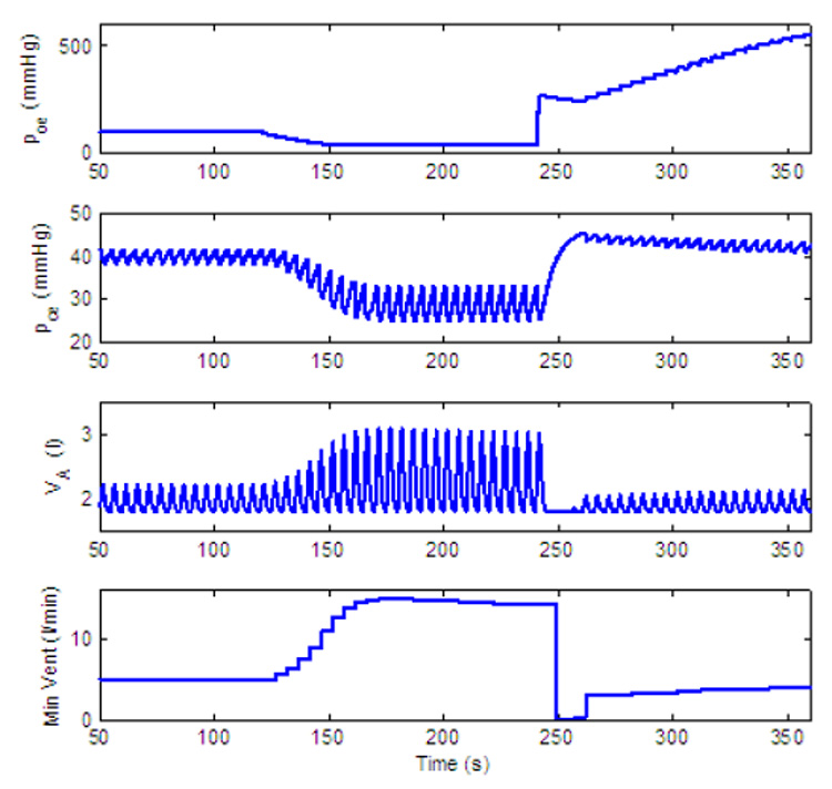
Dynamic response to inspired CO2 of a PI-controller with amplitude and CO2 control only. gn = 13.2, Kn = 0.5, A2 = 0.05, C2 = 0.002. All the other parameters in the feedback functions are zero. For t < 120 s, fcm = 0%, for 120 ≤ t < 240 s, fcm = 7.5% and for t ≥ 240 s, fcm = 0%.
Fig. 19.
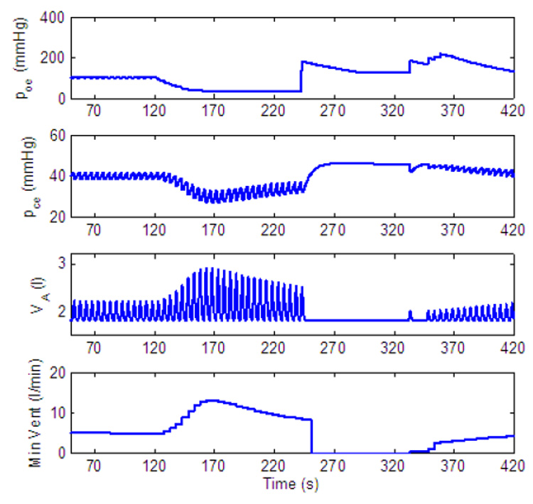
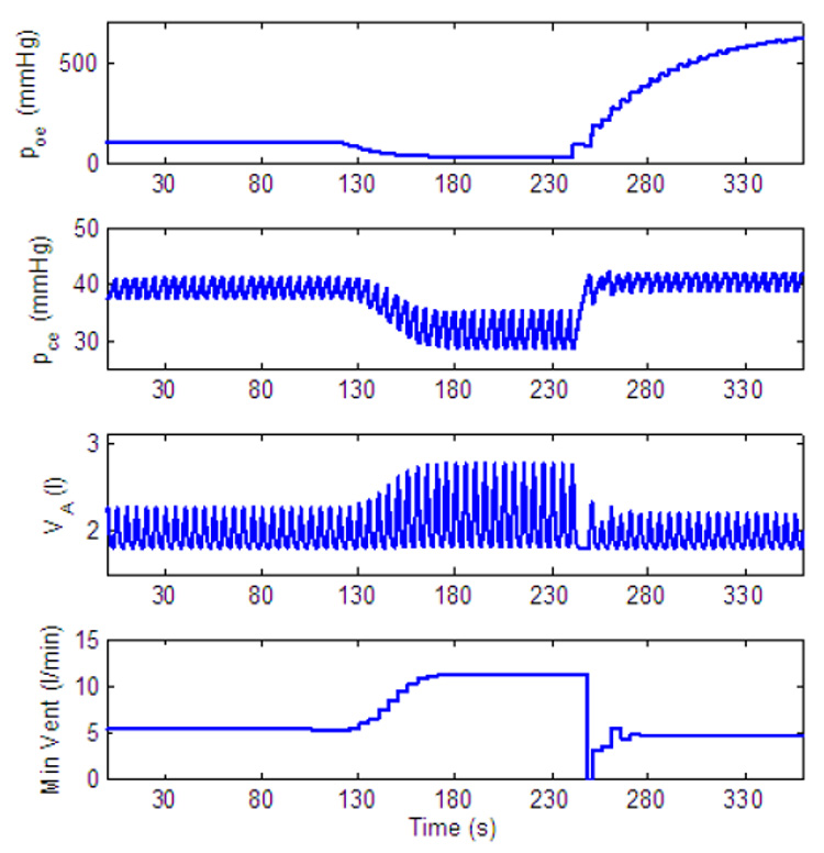
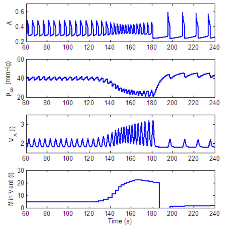
Dynamic response to decreased level of inspired O2 of a PI-controller with amplitude control only. gn = 13.2, Kn = 0.5, A2 = 0.05, B2 = 10, C2 = 0.002, D2 = 0.004. All the other parameters in the feedback functions are zero. For t < 120 s, fom = 21%, for 120 ≤ t < 240 s, fom = 5% and for t ≥ 240 s, fom = 100%.
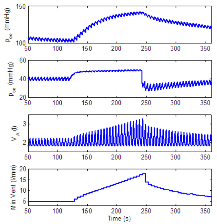
Fig. 20.
Dynamic response to decreased level of inspired O2 of a PI-controller with amplitude control only. gn = 13.2, Kn = 0.5, A2 = 0.05, B2 = 10, C2 = 0.002, D2 = 0.08. All the other parameters in the feedback functions are zero. For t < 120 s, fom = 21%, for 120 ≤ t < 240 s, fom = 5% and for t ≥ 240 s, fom = 100%.
Fig. 23.
Dynamic response to increased level of inspired CO2 of a P-controller with frequency and CO2 control only. gn = 13.2, Kn = 0.5, A1 = 0.5. All the other parameters in the feedback functions are zero. For t < 120 s, fcm = 0%, for 120 ≤ t < 240 s, fcm = 7.5% and for t ≥ 240 s, fcm = 0%.
Fig. 24.
Dynamic response to inspired CO2. Control of both amplitude and frequency. gn = 13.2, Kn = 0.5, A2 = 0.05, C2 = 0.002, C1 = 0.01. All the other parameters in the feedback functions are zero. For t < 60 s, fcm = 0%, for t ≥ 60 s, fcm = 7.5%.
Fig. 25.
Dynamic response to decreased level of inspired O2 - another mechanism for apnea appearance. gn = 13.2, Kn = 0.5, B1 = 30, B2 = 10, C1 = 0.01. All the other parameters in the feedback functions are zero. For t < 120 s, fom = 21%, for 120 ≤ t < 180 s, fom = 5% and for t ≥ 180 s, fom = 100%.
4 Results
The integrated model consists of nine ordinary differential equations. These equations were solved simultaneously using the subroutine Radau5 (this is an implicit Runge-Kutta method of order 5, available online, http://www.unige.ch/~hairer/software.html). We first show the dynamic response with an open loop control where the control parameters and K=Kn are set values. We then study the dynamic response of the model to changes in the concentration of inspired O2 or inspired CO2 for different feedback signals.
4.1 Open loop control
4.1.1 Existence of two regimes
Fig. 10 shows the steady-state solutions of lung volume for three different values of gn and Kn (nominal values of and K respectively). The blue (solid) line represents nominal values, the red (dashed) line represents variation in gn and the green (dashed-dotted) line represents variations in Kn. As can be seen the control model is capable of having two regimes (both seen under different physiological conditions), one in which an increased frequency is accompanied by a decreased amplitude (when only is varied) and another in which an increased frequency is accompanied by an increased amplitude (when both and K are varied).
Fig. 10.
Open loop control. Solid (blue) line: gn = 13.2, Kn = 0.5. Dashed (red) line: gn = 7, Kn = 0.5. Dashed-doted (green) line: gn = 13.2, Kn = 0.7.
4.1.2 Effects on minute ventilation
Fig. 11 and Fig. 14 show the effect of variation in gn and Kn on minute ventilation. The minute ventilation was calculated as Vi at the end of inspiration (see Eq. 10) divided by the respiration period. The relationship between Kn and the minute ventilation (Fig. 14) is linear (as can be expected) but the relationship between gn and the minute ventilation (Fig. 11) is nonlinear. Fig. 12 shows that as gn increases, the frequency increases monotonically; however as shown in Fig. 13, at the same time the tidal volume is decreasing. As a result, for some values of gn, increasing the frequency will lead to an increase in minute ventilation while a further increase in gn will result in a decrease in minute ventilation.
Fig. 11.
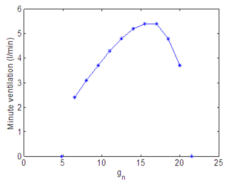
Effect of variation in gn on minute ventilation. Kn = 0.5.
Fig. 14.
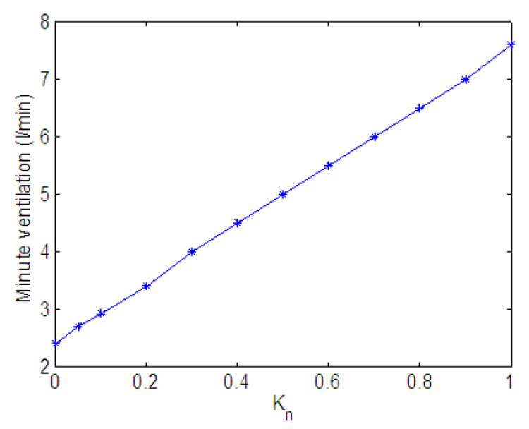
Effect of variation in Kn on minute ventilation. gn = 13.2.
Fig. 12.
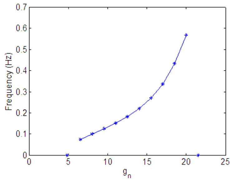
Effect of variation in gn on frequency. Kn = 0.5.
Fig. 13.
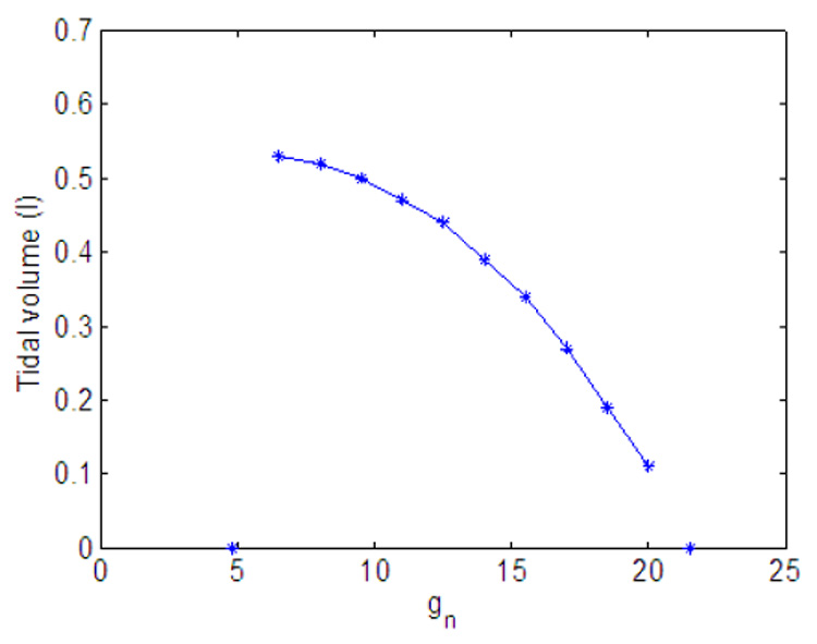
Effect of variation in gn on tidal volume. Kn = 0.5.
4.1.3 Open loop control output
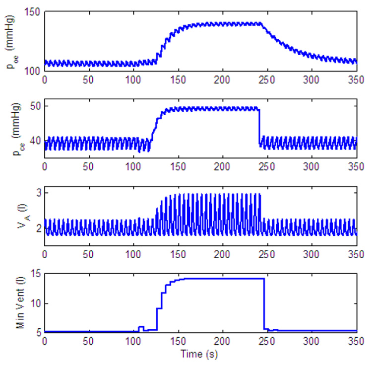
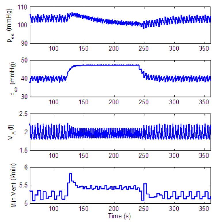
Fig. 15 shows the lung volume, the minute ventilation, and the blood partial pressures of oxygen and carbon dioxide at the end of the capillary, for a particular choice of parameters. We chose parameters that are close to physiological values. Parameters for the lung compartment are the same as in (Ben-Tal, 2006). The value of gn was chosen such that the period of the respiratory cycle (start of one inspiration to the next) would be 5 s. We chose the value of Kn such that the blood partial pressures of oxygen and carbon dioxide would be close to physiological values. Parameter values for the pre-BötC oscillator are based on (Purvis et al., 2007) (these values were scaled as described in Appendix B and Appendix C). Parameters for the muscle compartment were chosen such that the pleural pressure would have physiological values. It is important to emphasize that we have not tried to fit all the parameters at the same time to mimic a specific experiment and that the parameters in the model we propose can be estimated for each compartment based on independent experiments. The parameters we have chosen for the open loop control model were kept constant when the feedback control was studied.
Fig. 15.
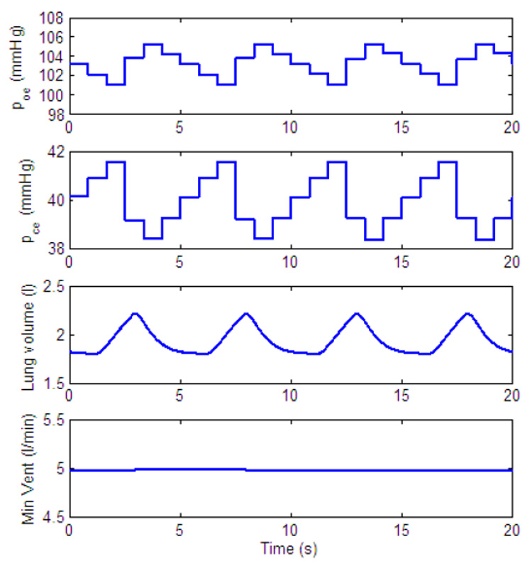
Output of open loop control. poe and pce are the blood partial pressures of oxygen and carbon dioxide, respectively, at the end of the capillary. Their values are updated every heart beat. gn = 13.2, Kn = 0.5. All the other parameters in the feedback functions are zero.
4.2 Closed loop control
It is well known that when increased levels of CO2 or decreased levels of O2 are inspired the minute ventilation increases. However, it is not clear how much of this is due to variation in amplitude and how much is due to variation in frequency. The response varies between individuals, species and state (sleep, awake, anesthetized). For example, in response to increased levels of CO2; both amplitude and frequency increased in awake humans (Dripps and Comroe, 1947a), in humans during r.e.m sleep (Berssenbrugge et al., 1983), in anesthetized dogs (Comroe, 1977), in anesthetized rats (Martin-Body and Sinclair, 1987, 1985; Zhou et al., 1996), and in awake rats (Walker et al., 1985). The increase in amplitude was more dominant in humans during non-r.e.m sleep (Berssenbrugge et al., 1983), in awake rats (Maskrey et al., 1981; Zhou et al., 1996) and in awake hamsters (Walker et al., 1985). In some cases the increase in frequency was more dominant (awake rat Martin-Body and Sinclair, 1985) and in other cases there was a decrease in frequency (awake hamster Walker et al., 1985).
In response to decreased levels of O2 both amplitude and frequency increased in awake humans (Comroe, 1977), in awake rats (Walker et al., 1985) and in anesthetized dogs (Comroe, 1977). The increase in amplitude was more dominant in awake humans (Dripps and Comroe, 1947b) while the increase in frequency was more dominant in awake rats (Maskrey et al., 1981) and in awake hamsters (Walker et al., 1985). In some cases inhaling decreased levels of O2 resulted in periodic breathing in humans during non-r.e.m sleep (Berssenbrugge et al., 1983).
It is possible that the different (and sometimes contradicting) responses can all exist in the control system under slightly different sets of parameters. We therefore did not try to fit the feedback parameters to a particular experiment. Instead we study the response to amplitude and frequency control separately for different feedback control signals and we identify qualitative differences in these responses.
4.2.1 Amplitude control
We study the dynamic response of different controllers by mimicking two experiments described by Comroe (1977). In the first experiment normal con-centration of gas (0% CO2, 21% O2) is inhaled for t < 120 s, 7.5% CO2 is inhaled for 120 ≤ t < 240 s, and 0% CO2 is inhaled again for t ≥ 240 s. In the second experiment normal concentration of gas (0% CO2, 21% O2) is inhaled for t < 120 s, 5% O2 is inhaled for 120 ≤ t < 240 s, and 100% O2 is inhaled for t ≥ 240 s. Fig. 16 and Fig. 18 mimic the first experiment (increased inspired concentrations of CO2) while Fig. 17, Fig. 19 and Fig. 20 mimic the second experiment (reduced inspired concentrations of O2). In Fig. 16 and Fig. 17 a P-controller is used while a PI-controller is used in Fig. 18, Fig. 19 and Fig. 20. Feedback control for CO2 only is used to study the dynamic response of inhaled CO2 and feedback control for CO2 and O2 is used to study the dynamic response of inhaled O2. We also show how minute ventilation changes in response to increased CO2 (Fig. 21) and decreased O2 (Fig. 22) when both CO2 and O2 are controlled.
Fig. 21.
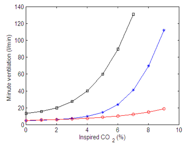
Minute ventilation as a function of inspired CO2. Calculated at the end of 200 s. Red (circle) line - P controller, gn = 13.2, Kn = 0.5, A2 = 0.2, B2 = 10. All the other parameters in the feedback functions are zero, inspired O2 is 21%. Blue (star) line - PI controller, gn = 13.2, Kn = 0.5, A2 = 0.05, B2 = 10, C2 = 0.002, D2 = 0.08. All the other parameters in the feedback functions are zero, inspired O2 is 21%. Black (square) line - PI controller, same parameters as for the blue line, inspired O2 is 5%.
Fig. 22.
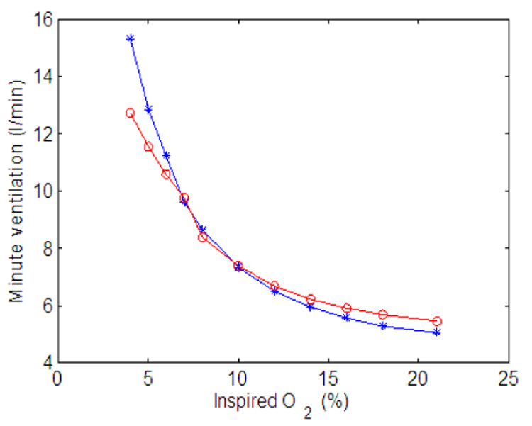
Minute ventilation as a function of inspired O2. Claculated at the end of 500 s. Red (circle) line - P controller, gn = 13.2, Kn = 0.5, A2 = 0.2, B2 = 10. All the other parameters in the feedback functions are zero. Blue (star) line - PI controller, gn = 13.2, Kn = 0.5, A2 = 0.05, B2 = 10, C2 = 0.002, D2 = 0.08. All the other parameters in the feedback functions are zero.
As can be seen in Fig. 16 and Fig. 18 the amplitude increases in response to an increased concentration of inspired CO2 and returns to normal when normal concentrations of CO2 are inspired for both types of controllers. However, the response is slower in the PI-controller. This is in agreement with Comroe (1977) who emphasizes that the tidal volume increases slowly. Another qualitative difference in the dynamic response of the two controllers is that steady state is reached in Fig. 16 (P-controller) while steady state is not reached in Fig. 18 (PI-controller). The reason for this can be explained as follows (see also Parr, 1996). By differentiating Eq. (13) for K we get
| (14) |
When increased levels of CO2 are inspired Erc is increased (since pce > pcr) and the control system tries to eliminate the error by increasing the amplitude. These efforts however are in vain (since the neural system has no control over the inspired concentration of CO2) and Erc reaches a steady state other than zero. When a P-controller is used C2 = 0 and a steady state in Erc will lead to a steady state in K (see Eq. (14)). But for a PI-controller (where C2 ≠ 0) K will keep increasing.
When both CO2 and O2 are controlled Eq. (14) becomes
| (15) |
When inspired CO2 is inhaled the control system tries to eliminate Erc by increasing the amplitude. As a result there is an increase in the levels of O2 and a positive Ero is created. For a P-controller (where C2 = D2 = 0) the system reaches steady state once the errors reach steady state. But for a PI-controller steady state can be reached only if
| (16) |
This balance can be achieved until hemoglobin reaches saturation and from that point on the system cannot reach steady state and K will keep increasing. For this reason the minute ventilation in Fig. 21 was calculated at the end of 200 s periods. In the numerical experiment that lead to Fig. 21 we changed the concentrations of CO2 in intervals of 200 s without allowing the system to go back to normal breathing before a change took place. This experiment is therefore similar to a rebreathing experiment where a person rebreathes into a sac of gas (filled with an initial higher concentration of oxygen) thereby causing the concentration of CO2 to change continuously. As can be seen in Fig. 21 there is a large difference between the response produced by the P-controller (red circle line) and the response produced by the PI-controller (blue star line). The response produced by the PI-controller is consistent with experiments (see for example Comroe, 1977; Kellogg, 1964). The shift to the left when 5% O2 is inhaled (green square line, produced by a PI-controller) is also consistent with experiments (see for example Kellogg, 1964) and can be explained by Eq. (15) since then Ero is negative and is larger.
When reduced concentrations of O2 are inspired Ero is negative and the amplitude will initially increase. As a result Erc will also become negative. For a P-controller (for which C2 = D2 = 0) a steady state in the errors will lead to a steady state in K and in the amplitude as can be seen in Fig. 17. For a PI-controller |Erc| can increase enough to cause the amplitude to decrease until the balance in Eq. (16) is achieved. This is illustrated in Fig. 19 (where the amplitude is decreased after an initial increase) and in Fig. 20 (where steady state is reached at a higher amplitude by increasing D2).
Once 100% O2 is administrated all three controllers in Fig. 17, Fig. 19 and Fig. 20 show an apnea. Apnea (cessation of breathing in the resting expiratory position, Comroe, 1977) is a characteristic dynamical response of the respiratory system in this type of experiment (Comroe, 1977). Our model suggests that the apnea is the result of the sudden removal of the term B2Ero in Eq. (13) and the fact that due to Erc, K is suddenly below the threshold for ramp integration. The P-controller in Fig. 17 recovers quickly and respiration resumes. While the longest apnea is seen in Fig. 19 where, due to the integration over Erc, the recovery takes longer. This longer apnea is consistent with (Comroe, 1977). When D2 is increased the change in K is not as abrupt as in Fig. 19 and the apnea is shorter in Fig. 20.
Minute ventilation as a function of O2 concentration is shown in Fig. 22. The numerical experiment was done in a similar way to the CO2 experiment except that the minute ventilation was calculated at the end of 500s to make sure it is in steady state. The response is similar for both the P-controller and the PI-controller. In both cases there is a larger increase for low concentrations of O2 but not as much as seen experimentally. This could be improved by adding the control of frequency (resulting in increased minute ventilation due to an increase in both frequency and amplitude).
4.2.2 Frequency control
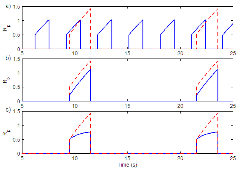
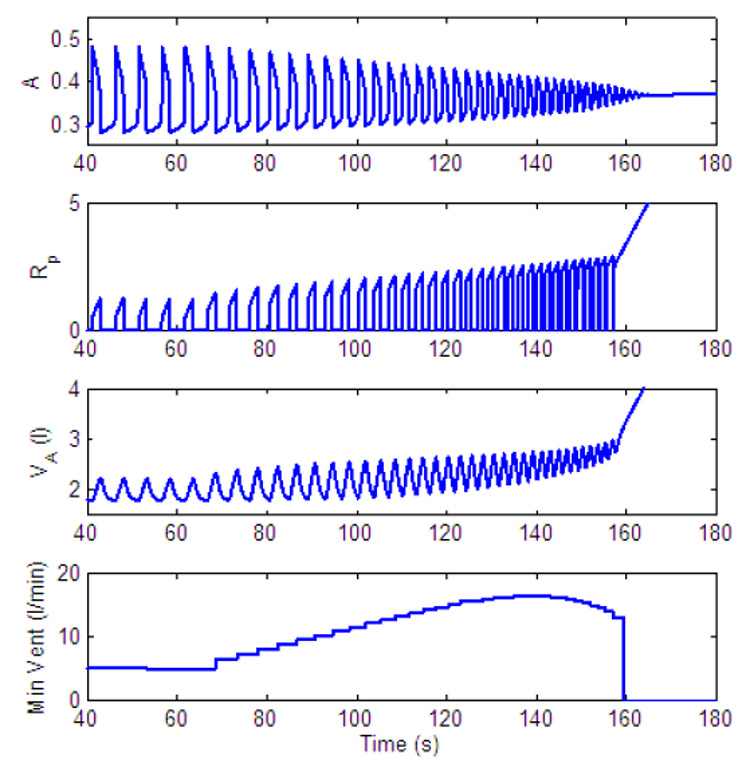
The discussion on the differences between a P-controller and a PI-controller given in the previous subsection holds also for frequency control. Here we illustrate some of the limitations and predictions of the model in regards to frequency control. Fig. 23 shows the response of a P-controller when only frequency and CO2 are controlled. As can be seen in this figure and as was illustrated in Fig. 11, the increase in minute ventilation is limited with frequency control. Fig. 23 also shows that when the gain (A2 in this case) in the feedback function is large enough oscillations start to appear in the minute ventilation.
Fig. 24 illustrates that both frequency and amplitude can be increased (initially) in the model. However, in our model, if a PI-controller is used for frequency control, the oscillator eventually reaches the beating state which leads to "holding the breath". This is a limitation of the current rhythm generator but could represent apneusis (cessation of breathing in the inspiratory position) under extreme physiological conditions (see for example Comroe, 1977).
Fig. 25 illustrates that there could be another mechanism for apnea appearance when Ero is suddenly removed from the feedback function for by administrating 100% O2 following a period of inspired 5% O2, thereby moving the pre-BötC into a silent mode.
5 Discussion and conclusions
We developed an integrated model of the respiratory neurochemical control system that incorporates essential aspects of the dynamical operation of brain-stem respiratory circuits, coupled to models of lung mechanics, gas exchange and blood gas transport with feedback regulation of oxygen and carbon dioxide. Our neural model has incorporated separate mechanisms for oscillatory activity generation and generation of ramp inspiratory activity patterns in a configuration that allows for independent control of inspiratory frequency and the amplitude of inspiratory neural drive to the lung diaphragm. This inde-pendent control is an essential property exhibited by the neural controller but has not been explicitly incorporated in other recent attempts to couple simplified non-dimensional neural activity-type models with neurochemical feedback control (e.g. Longobardo et al., 2005).
We represented the rhythm generation oscillator by a known biophysical mechanism that incorporates intrinsic dynamics of the pre-BötC. This mechanism allows for frequency control by input drives over a wide dynamic range, as well as multi-state behavior (no activity, oscillations, and tonic activity) as exhibited by the pre-BötC. The oscillator used in the model has a reduced set of inputs. However, our activity model can be expanded to explicitly incorporate other “interaction” terms in Eq. (1) to represent specific types of neural synaptic interactions (e.g. phasic inhibitory inputs) seen in the intact system at the level of the pre-BötC. However a full analysis of the dynamics of a more complex oscillator structure including its control by input signals will be required before such models can be usefully incorporated into an integrated control model.
We have represented the transformation of the drive from the pre-BötC oscillator into a ramping neural signal as a leaky integration process. We illustrated in Fig. 5 that the amount of leak can affect the shape of the ramp. These different activity patterns are seen experimentally. We have also shown in Fig. 6 how the amplitude at the neural level can be controlled in our model. These three mechanisms for amplitude control are also seen experimentally, but we adopted the most prominent mechanism involved in amplitude control by CO2. While the feedback control function we have implemented affected the external drives to the pre-BötC and the ramp generator, it did not affect the leak in the integrator. This can be implemented if required when more information becomes available on the effect of CO2 and O2 concentrations in the blood on pattern formation at the neural level.
The reduced neural model has been coupled to lung models that have been previously developed (Ben-Tal, 2006). To couple the models we had to introduce a simplified description of muscle mechanics (see Section 3.1). The model output we obtained for the pleural pressure is a non-symmetric signal, consistent with experimental observations. This differentiates between our model, which mimics the real system more closely, and previous models where the pleural pressure has been taken as a sinusoidal function.
We have studied the coupled system under open loop control in Section 4.1 and shown that two regimes can exist in the model, one in which an increased frequency is accompanied by a decreased amplitude and one in which an increased frequency is accompanied by an increased amplitude. We also studied how the external drives to the neural controller affect the minute ventilation and showed that while the drive to the pre-BötC increases the frequency monotonically it decreases the amplitude at the same time. As a result the increase in minute ventilation associated with the increase in frequency is limited. Thus the dynamics of the pre-BötC network are limiting in terms of amplitude control, but this limitation is overcome by implementing independent amplitude control downstream from the oscillator. Thus in our model, minute ventilation can be increased significantly by changes in amplitude and is not limited in the system.
The dynamics of the control signals related to the controlled variables (oxygen and carbon dioxide) as well as how these signals operate at the level of the neural system are poorly understood. While we did not explicitly take into account dynamics of the chemoreceptors themselves, we nevertheless included this implicitly by adopting several standard feedback controllers, specifically P- and PI- controllers, from control theory. We allowed control of both fre-quency and amplitude by the feedback functions through the external drives and used the open loop output to tune the nominal values of the feedback function. We then analyzed the output of the integrated system and compared the performances of the different controllers qualitatively.
The PI-controller gave results that fit better with experimental data. In Fig. 21 the nonlinear curve of minute ventilation as a function of inspired CO2 produced by the PI-controller is in agreement with (Dripps and Comroe, 1947a). The transient time in response to changes of inspired CO2 is slower in the PI- controller than it is in the P-controller, and in Fig. 19 long apnea appears when 100% O2 is inhaled following 5% O2. This is in agreement with experiments reported in (Comroe, 1977).
We have explained why the PI-controller cannot reach steady state when only CO2 is controlled (in the inspired CO2 experiment) and once hemoglobin saturation is reached when both CO2 and O2 are controlled. This new prediction of our model, seen in Fig. 18 and which also explains the nonlinear response in Fig. 21, needs to be verified experimentally but we note that Dripps and Comroe (1947a) reported that "Plateaus for minute volume were reached in only 27 of 42 individuals breathing 7.6 per cent CO2 ‥‥ and in 13 of 31 subjects inhaling 10.4 per cent CO2 ‥‥".
Our model predicts that there could be two possible mechanisms for apnea appearance. One via the amplitude control mechanism as seen in Fig. 19 and one via frequency control as seen in Fig. 25. This prediction also needs to be verified experimentally.
Our current model can be driven into apneusis when the coefficients in the control function are too large as can be seen in Fig. 24. This is not necessarily the behaviour of the neurological system under normal conditions but could represent pathological conditions where termination of inspiration is abnormal (e.g. Richter et al., 2003).
The model we have presented in this paper is the first step towards unified models for the respiratory system. There are several features we have not included in this model such as delays in the circulatory system and mechanosensory feedback via pulmonary stretch receptors. These features can be easily incorporated into the model as indicated in Section 2.2 and Section 3.2 but detailed analysis of the effect they have on the model’s dynamic behavior requires a separate study that will be conducted in the future. Despite the missing features, our model highlights important issues in amplitude and frequency control and in controlling the competing signals of CO2 and O2 regulation.
6 Acknowledgement
We would like to thank Dr. Ilya Rybak and Dr. Lorin Milescu for their useful suggestions. This research was supported by a Marsden Fund from the Royal Society of New Zealand and the Intramural Research Program of NINDS, NIH.
Appendix
A Appendix: parameters and variables
This appendix lists the parameters and variables that appear frequently in the paper (unless a different value is given in the text). The variables are listed in Table 1 and the parameters are listed in Table 2.
Table 1.
| Variables | |
|---|---|
| Symbol | Meaning |
| A | Activity of the pre-BötC population |
| hp | Inactivation gating of persistent sodium |
| R(t) | Ramp signal (phrenic activity) |
| xm | Muscle displacement |
| PL | Pleural pressure |
| PA | Alveolar total pressure |
| pao | Alveolar partial pressure of O2 |
| pac | Alveolar partial pressure of CO2 |
| po | Blood partial pressure of O2 |
| pc | Blood partial pressure of CO2 |
| fo | Concentration of O2 in alveoli |
| fc | Concentration of CO2 in alveoli |
| VA | Lung volume |
| q | Air flow through the airways |
| z | Concentration of |
| t | Time (Independent variable) |
Table 2.
| Parameters | ||
|---|---|---|
| Symbol | Meaning | Value (Ref) |
| Activating rate constant of A | 133.33 s−1 (See Appendix B) | |
| Inactivating rate constant of A | 98 s−1 (See Appendix B) | |
| gn | Nominal value of the control parameter | 5 – 22* s−1 (See Appendix B) |
| Parameter affecting | 0.367 (See Appendix B) | |
| Parameter affecting | −0.033 (See Appendix B) | |
| Parameter affecting hp | 0.313 (See Appendix B) | |
| Parameter affecting hp | 0.04 (See Appendix B) | |
| Parameter affecting hp | 10 s (See Appendix B) | |
| ã | Scaling parameter | 6.6667 V−1 |
| b̃ | Scaling parameter | 0.6667 |
| Parameter affecting the external drive of A | 0.212 (See Appendix B) | |
| k1 | Recoil rate constant of muscle | 2 s−1 |
| k2 | Conversion constant | 1 m · s−1 |
| kp | Conversion constant | 2.5 mmHg · m−1 |
| PL0 | Constant related to pleural pressure | 4.5 mmHg (Comroe, 1977) |
| Pm | Mouth total pressure | 760 mmHg (Ben-Tal, 2006) |
| Pw | Vapor pressure of water at 37°C | 47 mmHg (Ben-Tal, 2006) |
| fom | Concentration of O2 in the mouth | 0.21 (Ben-Tal, 2006) |
| fcm | Concentration of CO2 in the mouth | 0 (Ben-Tal, 2006) |
| V0 | Volume of the lungs when fully collapsed | 0 l (Ben-Tal, 2006) |
| VD | Lung dead space | 0.15 l (Ben-Tal, 2006) |
| Vc | Capillaries volume | 0.07 l (Ben-Tal, 2006) |
| R | Airways resistance to flow | 1 mmHg · s · l−1(Ben-Tal, 2006) |
| E | Lung elastance | 2.5 mmHg · l−1 (Ben-Tal, 2006) |
| TL | Time between heart beats | 60/72 s (Ben-Tal, 2006) |
| Do | Diffusion capacity of O2 | 3.5 × 10⁻⁴ l · s−1 · mmHg−1 |
| = 1.56 × 10⁻⁵ mol · s−1 · mmHg−1 | (Ben-Tal, 2006) | |
| Dc | Diffusion capacity of CO2 | 7.08 × 10⁻³ l · s−1 · mmHg−1 |
| = 3.16 × 10⁻⁵ mol · s−1 · mmHg−1 | (Ben-Tal, 2006) | |
| σ | Solubility of O2 in plasma | 1.4 × 10⁻⁶ mol · l−1 · mmHg−1(Ben-Tal, 2006) |
| σc | Solubility of CO2 in plasma | 3.3 × 10⁻⁵ mol · l−1 · mmHg−1(Ben-Tal, 2006) |
| Th | Concentration of hemoglobin molecule | 2 × 10⁻³ mol · l−1 (Ben-Tal, 2006) |
| KT | Equilibrium constants in the saturation function of hemoglobin | 10 × 103 l · mol−1 (Ben-Tal, 2006) |
| KR | 3.6 × 10⁶ l · mol−1 (Ben-Tal, 2006) | |
| L | 171.2 × 10⁶ (Ben-Tal, 2006) | |
| h | Concentration of H+ | 10−7.4 mol · l−1 (Ben-Tal, 2006) |
| r2 | Dehydration reaction rate | 0.12 s−1 (Ben-Tal, 2006) |
| l2 | Hydration reaction rate | 164 × 103 l · s−1 · mol−1 (Ben-Tal, 2006) |
| δ | Acceleration rate | 101.9(Ben-Tal, 2006) |
Range for which breathing occurs
B Appendix: Comparison with the Butera model
The normalized parameters in this model were compared to parameters in a modified version of Model 1 in (Butera et al., 1999a). As can be seen in Table 3 all the parameter values are exactly the same or very similar to parameter values in (Purvis et al., 2007). gL and EL were adjusted to make the breathing rate and the ratio between inspiratory time and expiratory time similar to those seen in humans under normal conditions.
Table 3.
| Butera model (Purvis et al., 2007) | This model |
|---|---|
| c = 21 × 10−12 (F) | – |
| gnap = 1 – 4 × 10⁻⁹ (S) | |
| gL = 1 – 4 × 10⁻⁹ (S) | |
| gt = 0.1 – 0.5 × 10⁻⁹ (S)* | gt = gnc = 0.1 – 0.5 × 10⁻⁹ (S)* |
| Enap = 50.0 × 10⁻³ (V) | |
| EL = −70.0 × 10⁻³ (V) | |
| θmp = −45.0 × 10⁻³ (V) | |
| σmp = −5.0 × 10⁻³ (V) | |
| θhp = −53.0 × 10⁻³ (V) | |
| σhp = 6.0 × 10⁻³ (V) | |
Range of values for which bursting appears.
C Appendix: Relationship between an activity model and a voltage-based model
The population activity, A, can be related to the average voltage, υ, by using the transformation (Tabak and Rinzel, 2005)
Equation (1) then becomes:
where is the current of persistent sodium, gL (υ − EL) is the leak current and gtυ is the tonic drive. The voltage-based population model has been studied by Rubin and Terman (2002).
Footnotes
Publisher's Disclaimer: This is a PDF file of an unedited manuscript that has been accepted for publication. As a service to our customers we are providing this early version of the manuscript. The manuscript will undergo copyediting, typesetting, and review of the resulting proof before it is published in its final citable form. Please note that during the production process errors may be discovered which could affect the content, and all legal disclaimers that apply to the journal pertain.
References
- Batzel JJ, Kappel F, Schneditz D, Tran HT. Cardiovascular & Respiratory Systems: Modeling, Analysis & Control. Frontiers in Applied Mathematics. SIAM. 2006 [Google Scholar]
- Batzel JJ, Tran HT. Modeling instability in the control system for human respiration: applications to infant non-REM sleep. Appl. Math. Comput. 2000;110:1–51. [Google Scholar]
- Ben-Tal A. Simplified models for gas exchange in the human lungs. Journal of Theoretical Biology. 2006;238:474–495. doi: 10.1016/j.jtbi.2005.06.005. [DOI] [PubMed] [Google Scholar]
- Berssenbrugge A, Dempsey J, Iber C, Skatrud J, Wilson P. Mechanisms of hypoxia-induced periodic breathing during sleep in humans. Journal of physiology. 1983;343:507–524. doi: 10.1113/jphysiol.1983.sp014906. [DOI] [PMC free article] [PubMed] [Google Scholar]
- Butera RJ, Rinzel J, Smith JC. Models of respiratory rhythm generation in the pre-bötzinger complex. I. bursting pacemaker neurons. Journal of Neurophysiology. 1999a;81:382–397. doi: 10.1152/jn.1999.82.1.382. [DOI] [PubMed] [Google Scholar]
- Butera RJ, Rinzel J, Smith JC. Models of respiratory rhythm generation in the pre-bötzinger complex. II. populations of coupled pacemaker neurons. Journal of Neurophysiology. 1999b;81:398–415. doi: 10.1152/jn.1999.82.1.398. [DOI] [PubMed] [Google Scholar]
- Carley DW, Shannon DC. A minimal mathematical model of human periodic breathing. J. Appl. Physiol. 1988;65(3):1400–1409. doi: 10.1152/jappl.1988.65.3.1400. [DOI] [PubMed] [Google Scholar]
- Comroe JH. Physiology of respiration. 2nd Edition. Year Book Medical Publishers, Inc.; 1977. [Google Scholar]
- D’angelo E, Sant’ambrogio G, Agostoni E. Effect of diaphragm activity or paralysis on distribution of pleural pressure. J. Appl. Physiol. 1974;37:311–315. doi: 10.1152/jappl.1974.37.3.311. [DOI] [PubMed] [Google Scholar]
- Del Negro CA, Johnson SM, Butera RJ, Smith JC. Models of respiratory rhythm generation in the pre-bötzinger complex. III. experimental tests of model predictions. Journal of Neurophysiology. 2001;86:59–74. doi: 10.1152/jn.2001.86.1.59. [DOI] [PubMed] [Google Scholar]
- Del Negro CA, Koshiya N, Butera RJ, Smith JC. Persistent sodium current, membrane properties and bursting behavior of pre-bötzinger complex inspiratory neurons in vitro. Journal of Neurophysiology. 2002;88:2242–2250. doi: 10.1152/jn.00081.2002. [DOI] [PubMed] [Google Scholar]
- Dripps RD, Comroe JH. The respiratory and circulatory response of normal man to inhalation of 7.6 and 10.4 per cent co2 with a comparison of the maximal ventilation produced by severe muscular exercise, inhalation of co2 and maximal voluntary hyperventilation. American journal of Physiology. 1947a;149:43–51. doi: 10.1152/ajplegacy.1947.149.1.43. [DOI] [PubMed] [Google Scholar]
- Dripps RD, Comroe JH. The effect of the inhalation of high and low oxygen concentrations on respiration, pulse rate, ballistocardiogram and arterial oxygen saturation (oximeter) of normal individuals. American journal of Physiology. 1947b;149:277–291. doi: 10.1152/ajplegacy.1947.149.2.277. [DOI] [PubMed] [Google Scholar]
- Eldridge FL. The north carolina respiratory model. A multipurpose model for studying the control of breathing. In: Khoo MCK, editor. Bioengineering approaches to pulmonary physiology and medicine. New York: Plenum Press; 1996. pp. 25–49. [Google Scholar]
- Feldman JL. Neurophysiology of breathing in mammals. In: Bloom FE, editor. Handbook of Physiology - the Nervous System IV. Bethesda: American Physiological Society; 1986. pp. 463–524. [Google Scholar]
- Feldman JL, Smith JC. Neural control of respiratory pattern in mammals: An overview. In: Dempsey JA, Pack AI, editors. Regulation of Breathing. New York: Decker; 1995. pp. 39–69. [Google Scholar]
- Feldman JL, Smith JC, McCrimmon DR, Ellenberger HH, Speck DF. Generation of respiratory pattern in mammals. In: Cohen AH, Rossignol S, Grillner S, editors. Neural Control of Rhythmic Movements in Vertebrates. New York: Wiley; 1988. pp. 73–100. [Google Scholar]
- Fowler AC, Kalamangalam GP. Periodic breathing at high altitude. IMA J. Math. App. Med. 2002;19:293–313. [PubMed] [Google Scholar]
- Grodins FS, Buell J, Bart AJ. Mathematical analysis and digital simulation of the respiratory control system. J. Appl. Physiol. 1967;22(2):260–276. doi: 10.1152/jappl.1967.22.2.260. [DOI] [PubMed] [Google Scholar]
- Guyton AC, Hall JE. Textbook of Medical Physiology. 10th Edition. W B Saunders Company; 2000. [Google Scholar]
- Kellogg RH. Central chemical regulation of respiration. In: Fenn WO, Rahn H, editors. Handbook of Physiology, Respiration Vol. I. Washington DC: American Physiological Society; 1964. pp. 507–534. [Google Scholar]
- Khoo MCK, Yamashiro SM. Models of control of breathing. In: Chang M. P. HA, editor. Respiratory Physiology: An Analytical Approach. New York: Mercer Dekker; 1989. pp. 799–829. [Google Scholar]
- Longobardo G, Evangelesti C, Chernia NS. Introduction of respiratory pattern generators into models of respiratory control. Resp. Physiol. & Neurobi. 2005;148:285–301. doi: 10.1016/j.resp.2005.02.005. [DOI] [PubMed] [Google Scholar]
- Lu K, Clark JW, Jr, Ghorbel FH, Ware DL, Zwischenberger JB, Bidani A. Whole-body gas exchange in human predicted by a cardiopulmonary model. Cardiovascular Engineering. 2002 [Google Scholar]
- Martin-Body RL, Sinclair JD. Analysis of respiratory patterns in the awake and in the halothane anaesthetised rat. Respiration Physiology. 1985;61:105–113. doi: 10.1016/0034-5687(85)90032-5. [DOI] [PubMed] [Google Scholar]
- Martin-Body RL, Sinclair JD. Differences in respiratory patterns after acute and chronic pulmonary denervation. Respiration Physiology. 1987;70:205–219. doi: 10.1016/0034-5687(87)90051-x. [DOI] [PubMed] [Google Scholar]
- Maskrey M, Megirian D, Nicol SC. Effects of decortication and carotid sinus nerve section on ventilation of the rat. Respiration Physiology. 1981;43:263–273. doi: 10.1016/0034-5687(81)90108-0. [DOI] [PubMed] [Google Scholar]
- Monod J, Wyman J, Changeux J-P. On the nature of allosteric transitions: A plausible model. J. Mol. Biol. 1965;12:88–118. doi: 10.1016/s0022-2836(65)80285-6. [DOI] [PubMed] [Google Scholar]
- Parr EA. Control Engineering. Butterworth-Heinemann. 1996 [Google Scholar]
- Paton JFR, Abdala APL, Koizumi H, Smith JC, St-John WM. Respiratory rhythm generation during gasping depends on persistent sodium current. Nat. Neurosci. 2006;9:311–313. doi: 10.1038/nn1650. [DOI] [PubMed] [Google Scholar]
- Purvis LK, Smith JC, Koizumi H, Butera RJ. Intrinsic bursters increase the robustness of rhythm generation in an excitatory network. Journal of Neurophysiology. 2007;97:1515–1526. doi: 10.1152/jn.00908.2006. [DOI] [PubMed] [Google Scholar]
- Richter DW. Neural regulation of respiration: rhythmogenesis and afferent control. In: Gregor R, Windhorst U, editors. Comprehensive Human Physiology. Vol. II. Berlin: Springer-Verlag; 1996. pp. 2079–2095. [Google Scholar]
- Richter DW, Manzke T, Wilken B, Ponimaski E. Serotonin receptors: guardians of stable breathing. Trends in Mol. Med. 2003;9:542–548. doi: 10.1016/j.molmed.2003.10.010. [DOI] [PubMed] [Google Scholar]
- Rubin J, Terman D. Synchronized activity and loss of synchrony among heterogeneous conditional oscillators. SIAM journal of applied dynamical systems. 2002;1(1):146–174. [Google Scholar]
- Rybak IA, Paton JFR, Schwaber JS. Modeling neural mechanisms for genesis of respiratory rhythm and pattern: I. models of respiratory neurons. J. Neurophysiol. 1997a;77:1994–2006. doi: 10.1152/jn.1997.77.4.1994. [DOI] [PubMed] [Google Scholar]
- Rybak IA, Paton JFR, Schwaber JS. Modeling neural mechanisms for genesis of respiratory rhythm and pattern: II. network models of the central respiratory pattern generator. J. Neurophysiol. 1997b;77:2007–2026. doi: 10.1152/jn.1997.77.4.2007. [DOI] [PubMed] [Google Scholar]
- Rybak IA, Shevtsova NA, Paton JFR, Dick TE, St-John WM, Mörschel M, Dutschmann M. Modeling the ponto-medullary respiratory network. Resp. Physiol. & Neurobi. 2004;143:307–319. doi: 10.1016/j.resp.2004.03.020. [DOI] [PubMed] [Google Scholar]
- Saunders KB. A breathing model of the respiratory system: the controlled system. J. theor. Biol. 1980;84:135–161. doi: 10.1016/s0022-5193(80)81041-1. [DOI] [PubMed] [Google Scholar]
- Seung HS. Amplification, attenuation, and integration. In: Adbib MA, editor. The Handbook of Brain Theory and Neural Networks. 2nd edition. New York: Springer; 2003. pp. 183–215. [Google Scholar]
- Smith JC, Abdala APL, Koizumi H, Rybak IA, Paton JFR. Spatial and functional architecture of the mammalian brainstem respiratory network: a hierarchy of three oscillatory mechanisms. J. Neurophysiol. 2007 doi: 10.1152/jn.00985.2007. in Press (online) [DOI] [PMC free article] [PubMed] [Google Scholar]
- Smith JC, Butera RJ, Koshiya N, Negro CD, Wilson CG, Johnson SM. Respiratory rhythm generation in neonatal and adult mammals: The hybrid pacemaker-network model. Resp. Physiol. & Neurobi. 2000;122:131–147. doi: 10.1016/s0034-5687(00)00155-9. [DOI] [PubMed] [Google Scholar]
- Smith JC, Ellenberger HH, Ballanyi K, Richter DW, Feldman JL. Pre-bötzinger complex: A brainstem region that may generate respiratory rhythm in mammals. Science. 1991;254:726–729. doi: 10.1126/science.1683005. [DOI] [PMC free article] [PubMed] [Google Scholar]
- Tabak J, Rinzel J. Bursting in excitatory neural networks. In: Coombes S, Bressloff PC, editors. Bursting. The Genesis of Rhythm in the Nervous System. New Jersey: World Scientific; 2005. pp. 273–301. [Google Scholar]
- Topor ZL, Pawlicki M, Remmers JE. A computational model of the human respiratory control system: responses to hypoxia and hypercapnia. Ann. Biomed. Eng. 2004;32(11):1530–1545. doi: 10.1114/b:abme.0000049037.65204.4c. [DOI] [PubMed] [Google Scholar]
- Ursino M, Magosso E, Avanzolini G. An integrated model of the human ventilatory control system: the response to hypercapnia. Clin. Physiol. 2001a;21(4):447–464. doi: 10.1046/j.1365-2281.2001.00349.x. [DOI] [PubMed] [Google Scholar]
- Ursino M, Magosso E, Avanzolini G. An integrated model of the human ventilatory control system: the response to hypoxia. Clin. Physiol. 2001b;21(4):465–477. doi: 10.1046/j.1365-2281.2001.00350.x. [DOI] [PubMed] [Google Scholar]
- Walker BR, Adams EM, Voelkel NF. Ventilatory responses of hamsters and rats to hypoxia and hypercapnia. Journal of applied physiology. 1985;59(6):1955–1960. doi: 10.1152/jappl.1985.59.6.1955. [DOI] [PubMed] [Google Scholar]
- Zhou D, Huang Q, Fung M-L, Li A, Darnall RA, Nattie EE, John WMS. Phrenic response to hypercapnia in the unanesthetized decerebrate, newborn rat. Respiration Physiology. 1996;104:11–22. doi: 10.1016/0034-5687(95)00098-4. [DOI] [PubMed] [Google Scholar]