A diffusion model explanation of the worst performance rule for reaction time and IQ

Abstract

The worst performance rule for cognitive tasks [Coyle, T.R. (2003). IQ, the worst performance rule, and Spearman’s law: A reanalysis and extension. Intelligence, 31, 567–587] in which reaction time is measured is the result that IQ scores correlate better with longer (i.e., 0.7 and 0.9 quantile) reaction times than shorter (i.e., 0.1 and 0.3 quantile) reaction times. We show that this pattern of correlations can be predicted by the diffusion model [Ratcliff, R. (1978). A theory of memory retrieval. Psychological Review, 85, 59–108], in two ways: either assuming that the rate of accumulation of information toward a decision is higher for higher IQ subjects or assuming that the criterial amounts of information they require before a decision are lower. Importantly, the model explains both reaction times and accuracy, so the two possibilities can be distinguished.

In 2003, Coyle summarized evidence for the worst performance rule (Coyle, 2003). This rule describes the empirical finding that in a variety of cognitive tasks, trials on which performance is worst better predict general intelligence or IQ scores than trials on which performance is best. For reaction time (RT) studies, IQ scores usually correlate better with the slowest responses than the fastest responses, that is, better with higher quantile RTs than lower quantile RTs (Baumeister & Kellas, 1968; Diascro & Brody, 1993; Jensen, 1982; Kranzler, 1992; Larson & Alderton, 1990; but see Salthouse, 1998).

Although a number of explanations have been considered for the worst performance rule for RT, no investigations have examined predictions from a cognitive processing model that is designed to account for both accuracy and RT, including RT distribution shape, for both correct and error responses. The model examined in this article is the diffusion model for two-choice decisions (Ratcliff, 1978, 2002; Ratcliff & Rouder, 1998; Ratcliff, Van Zandt, & McKoon, 1999). This model has several advantages: first, the model explicitly fits RT distributions and so it can predict RT quantiles. Second, individual differences can be explicitly examined, and the model has been used extensively to do so. Third, the model allows two hypotheses to be evaluated about the locus of IQ effects: IQ is related to the quality of evidence extracted from a stimulus, or IQ is related to how conservatively decision criteria are set.

Fig. 1 illustrates the diffusion model. The model assumes that noisy information is accumulated over time toward one of two decision criteria. Three simulated paths are shown in Panel A. The rate of accumulation of information is termed the drift rate (v) and it is a function of the quality of stimulus information in perceptual judgments, the quality of match between a test item and memory in memory judgments, and so on. The decision process is assumed to start at a point z and accumulate evidence until a criterion at a or a criterion at 0 is reached. Variability with a trial gives rise to variability in RTs and allows the process to hit the wrong boundary giving rise to errors (the three jagged lines in Panel A). Panel B presents 40 simulated processes with drift rate driving the processes towards the top boundary. The paths are irregular and some hit the bottom boundary by mistake. The processes mainly finish quickly, they are bunched up to the left, but some finish more slowly, and this illustrates how variability in the model produces the right skewed RT distributions that are generally found in experimental results from two-choice tasks.

Fig. 1.

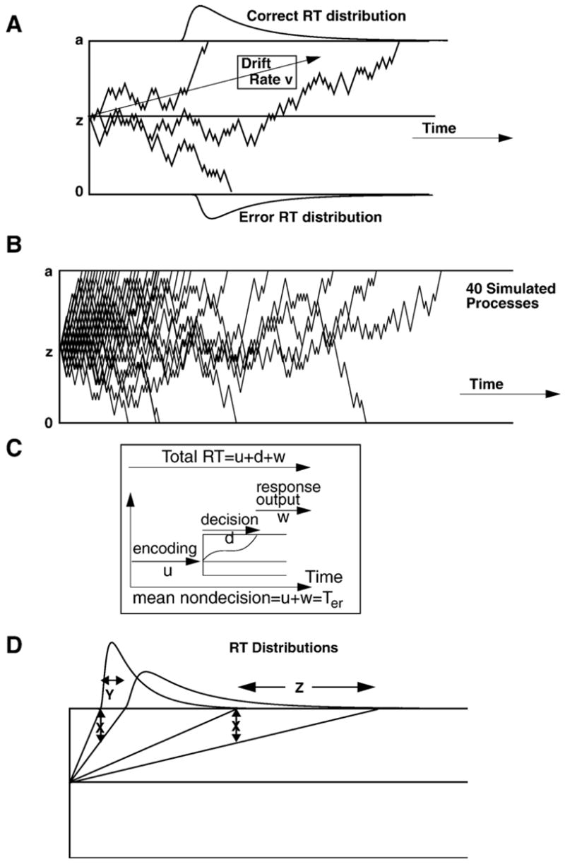
An illustration of the diffusion model. Panel A shows 3 simulated paths with drift rate v, boundary separation a, and starting point z. Panel B shows 40 diffusion processes simulated by a simple random walk — the discrete analog of the diffusion process. The starting point is at 10 and the top boundary at 20. There is a 0.58 probability of the process taking a step towards the top boundary. Panel C shows encoding (u), decision (d), and response output (w) processes with the nondecision components (mean=T_er) the sum of u and w. Panel D shows fast and slow processes from two drift rates which illustrate how an equal size slow down in drift rate (X) produces a small shift in the leading edge of the RT distribution (Y) and a larger shift in the tail (Z). Note that the components of processing are variable across trials with, ηrepresenting SD in drift across trials, s_z representing range of the distribution of starting point (z) across trials, and s_t representing range of the distribution of nondecision times across trials.

In addition to the decision process, the total RT includes other processes, such as stimulus encoding, memory access, and response output (illustrated in Panel C). These are combined and have a mean duration T_er.

Fig. 1, Panel D illustrates how RT distribution shape changes with stimulus difficulty, i.e., drift rate. The two processes on the left represent the fastest processes and those on the right, the slowest processes. If the drift rates for each of these are reduced by an amount “X”, the fastest responses increase by an amount “Y” and the slowest responses increase by an amount “Z” where Z is much larger than Y. This means that as drift rate changes, there is a small change in the leading edge of the RT distribution and a larger change in the tail.

It is assumed that the three main components of the model, namely, drift rate, boundary separation, and nondecision components of processing, have variability from trial to trial. The original motivation for this assumption (Ratcliff, 1978) was that it is unlikely that a subject can accurately hold components of processing constant from one trial to the next, or encode the same stimulus in exactly the same way on different trials. The assumption of trial to trial variability has the important consequence that the model can account for the behavior of error RTs relative to correct RTs including their distributions (Ratcliff & Rouder, 1998; Ratcliff & Smith, 2004; Ratcliff et al., 1999). Specifically, ηis the SD in normally distributed drift rates across trials (mean v), s_z is the range of a uniform distribution of starting points (mean z), and s_t is the range of a uniform distribution of times for the duration of nondecision components of processing (mean T_er). For further discussion of these assumptions, see Ratcliff and Tuerlinckx (2002).

There are explicit expressions for accuracy and the RT distribution probability density for the diffusion model, though the probability density involves an infinite sum of products of exponential and sine terms (Ratcliff & Smith, 2004, Eqs. A2 and A3) that requires numerical solutions. However there are no explicit or simple expressions when the drift rate, starting point, and nondecision components vary from trial to trial. To obtain predictions, three nested integrations must be performed over the infinite sum. This can be done by numerical methods, taking no more than a minute or two to fit the model to a standard set of data with, for example, 6 conditions (see Ratcliff & Tuerlinckx, 2002, Appendix B).

1. IQ and the diffusion model

To model how IQ affects RT, we examined how IQ might be related to one or more processing components of the diffusion model. If IQ were related to drift rate, an obvious possibility, people with higher IQ’s would extract higher quality evidence from stimuli, memory, and so on. If IQ were related to boundary separation, a perhaps less likely possibility, people with higher IQ might adjust their decision criteria to require less evidence before making a decision.

To examine these two possibilities, it was assumed that there is variability from one individual to another in their drift rates and boundary separations. Simulated data were generated for 1000 subjects with 200 observations per simulated subject. The correlations between the subjects’ drift rates and the quantiles of their RT distributions, as well as their accuracy, were examined. Likewise, the correlations between the subjects’ boundary separations and their data were examined. The main question was whether, with either source of across subject variability, the diffusion model would generate data that conformed to the worst performance rule. In other words, would the subjects’ drift rates or boundary separations correlate with RT quantiles, and would the correlation be stronger for the higher quantiles.

The simulated data were generated using parameter values typical of previous fits to data from experiments that examined the effects of aging on cognitive processing (e.g., recognition memory, lexical decision, perceptual tasks; Ratcliff, Thapar, Gomez, & McKoon, 2004; Ratcliff, Thapar, & McKoon, 2001, 2003, 2004; Thapar, Ratcliff, & McKoon, 2003). Drift rates (values of v) for individual subjects were selected from a normal distribution with mean v=0.4 and SD s_v =0.1 (in all but one simulation). Thus, this across trial variability in drift rates for the simulated subjects produced a range of values from about 0.2 to about 0.6 (2 SD’s on either side of v=0.4). Boundary separations (values of a) for individual subjects were selected from a normal distribution with mean 0.1 and SD (across subjects) either s_a =0.02 or 0.04, and nondecision components of processing for individual subjects were selected from a normal distribution with mean 0.4 and SD (across subjects) either s_Ter =0.05 or 0.10. These values of SD across subjects in boundary separation and nondecision components of processing span the range observed in experimental data.

2. Results

2.1. Drift rate and the worst performance rule

Table 1 shows results for nine sets of simulated data (1000 subjects per set). For the first three, the across trial variability parameters of the model (η, s_z, and s_t) were set to near 0.0 (0.001). In row 1 of the table, when there was no across subject variability in boundary separation (s_a =0) or the nondecision components (s_Ter =0), then drift rate correlated strongly positively with accuracy, and strongly negatively with mean RT and the five RT quantiles (the 0.1, 0.3, 0.5, 0.7, and 0.9 quantiles). The correlation increased and then decreased from the lower to the higher quantiles, forming a shallow inverted U. It might appear that this inverted U pattern is the result of a ceiling effect because the correlations were near 1, but row 2 of the table shows the same pattern when the correlations were not near ceiling. With the SD in drift across subjects reduced from 0.1 to 0.01, the correlation of drift rate with the 0.1 quantile was −0.06, rising to −0.22, and then decreasing to −0.19, again forming an inverted U shaped function.

Table 1.

Parameter values and correlations between drift rate (v) and data

Parameter values						Correlations with drift rate
Across subject			Within subject
sa	sv	sTer	η	sz	st	Acc.	$\overline{\text{RT}}$	Q 0.1	Q 0.3	Q 0.5	Q 0.7	Q 0.9
0.00	0.1	0.00	0.001	0.001	0.001	0.782	−0.919	−0.723	−0.856	−0.899	−0.900	−0.881
0.00	0.01	0.00	0.001	0.001	0.001	0.309	−0.255	−0.058	−0.187	−0.206	−0.224	−0.194
0.02	0.1	0.05	0.001	0.001	0.001	0.634	−0.354	−0.086	−0.188	−0.293	−0.401	−0.506
0.00	0.1	0.00	0.08	0.02	0.1	0.790	−0.925	−0.737	−0.843	−0.871	−0.908	−0.906
0.02	0.1	0.05	0.08	0.02	0.1	0.658	−0.455	−0.225	−0.288	−0.378	−0.476	−0.585
0.04	0.1	0.10	0.08	0.02	0.1	0.453	−0.223	−0.073	−0.110	−0.159	−0.234	−0.342
0.00	0.1	0.00	0.20	0.06	0.1	0.840	−0.810	−0.415	−0.557	−0.701	−0.771	−0.752
0.02	0.1	0.05	0.20	0.06	0.1	0.794	−0.246	−0.021	−0.072	−0.158	−0.269	−0.393
0.04	0.1	0.10	0.20	0.06	0.1	0.606	−0.106	−0.024	−0.036	−0.064	−0.108	−0.210

Note: Mean values of parameters fixed for every row of the table are: a=0.10, T_er =0.4, v =0.4. The parameters of the model are a =boundary separation, z=a/2=starting point, T_er =mean value of the nondecision components of response time, η=SD in drift across trials, s_z =range of the distribution of starting point (z) across trials, v =drift rate, and s_t =range of the distribution of nondecision times across trials. Variability in parameters across subjects: s_v variability in drift rate, s_a variability in boundary separation, and s_Ter variability in nondecision components of processing. Acc=accuracy, $\overline{\text{RT}}$=mean RT, and Q 0.1–Q 0.9 are the 0.1–0.9 quantile RTs.

For the results in the third row of Table 1, across subject variability in boundary separation and the non-decision components were added. With s_a =0.02 and s_Ter =0.05, the correlations between drift rate and accuracy and RTs were 0.63 for accuracy, −0.26 for mean RT, and −0.09 to −0.51 for the RT quantiles. The increase in the correlations from the lowest to the highest quantiles was almost linear, and so produced the worst performance rule.

The next six rows show what happens when across trial variability in drift rate, starting point, and the nondecision components was introduced (η, s_z, and s_t). When the across subject variability in s_a and s_Ter was zero, the correlations between drift rate and the RT quantiles showed the inverted U pattern (rows 4 and 7, Table 1). As the values of across subject variability in a and T_er increased, the correlations were reduced, but they were reduced more for the lower than for the higher quantiles, leading to a roughly linear increase. The correlations followed the worst performance rule in every case for which the across subject variability in a and T_er was greater than zero: the correlations increased approximately linearly from the 0.1 to the 0.9 quantile.

The first conclusion is that the diffusion model can produce correlations consistent with the worst performance rule. The correlations between drift rate and RT quantiles are negative and they increase from the lower to the higher quantiles. Second, while the correlations between drift rate and the quantiles are negative, the correlations with accuracy are positive. These conclusions hold as long as there is variability across subjects in a and T_er. Given that such variability is always obtained when the model is fit to large sets of data from individual subjects, the model automatically produces the worst performance rule.

2.2. Boundary separation and the worst performance rule

Although boundary separation might be a less plausible correlate of IQ than drift rate, it is important to understand what components of the model can give rise to the worst performance rule. Table 2 shows results for six sets of simulated data (1000 subjects per set). The across subject SD in boundary separation (s_a) was 0.01, 0.02, or 0.04, the across subject SD in drift rate (s_v) was 0.0 or 0.1, and the across subject SD in T_er (s_Te) was 0.0, 0.05 or 0.10. The across trial variability parameters (η, s_z, and s_t) were set near 0.0 for the data in the first two rows of the table and then increased for the other rows. When the across subjects variability parameters (s_v and s_Ter) were zero or near zero (the first row of the table), the correlation of quantile RTs with boundary separation decreased slightly with increasing quantiles, the opposite of the worst performance rule. But in all the other rows, the worst performance rule was obtained. Note that the correlations with the RT quantiles and accuracy were both positive, unlike the correlations with drift rate in which the correlations were of the opposite sign.

Table 2.

Parameter values and correlations between boundary separation (a) and simulated data

Parameter values						Correlations with boundary separation
Across subject			Within subject
sa	sv	sTer	η	sz	st	Acc.	$\overline{\text{RT}}$	Q 0.1	Q 0.3	Q 0.5	Q 0.7	Q 0.9
0.01	0.0	0.0	0.001	0.001	0.001	0.481	0.850	0.844	0.863	0.848	0.796	0.703
0.02	0.1	0.05	0.001	0.001	0.001	0.505	0.531	0.315	0.423	0.509	0.562	0.627
0.02	0.1	0.05	0.08	0.02	0.1	0.429	0.576	0.439	0.495	0.542	0.594	0.633
0.02	0.1	0.05	0.20	0.06	0.1	0.478	0.501	0.251	0.309	0.394	0.495	0.624
0.04	0.1	0.10	0.08	0.02	0.1	0.701	0.563	0.387	0.449	0.509	0.577	0.677
0.04	0.1	0.10	0.20	0.06	0.1	0.696	0.495	0.245	0.315	0.393	0.495	0.665

Note: Mean values of parameters fixed for every row of the table are: a=0.10, T_er =0.4, v =0.4. The parameters of the model are a =boundary separation, z=a/2=starting point, T_er =mean value of the nondecision components of response time, η=SD in drift across trials, s_z =range of the distribution of starting point (z) across trials, v=drift rate, and s_t =range of the distribution of nondecision times across trials. Variability in parameters across subjects: s_v variability in drift rate, s_a variability in boundary separation, and s_Ter variability in the mean value of the nondecision components of processing. Acc=accuracy, $\overline{\text{RT}}$=mean RT, and Q 0.1–Q 0.9 are the 0.1–0.9 quantile RTs.

3. Discussion

The results in Tables 1 and 2 show that the diffusion model generates data consistent with the worst performance rule if IQ is correlated with drift rate or if IQ is correlated with boundary separation, but only when other components of processing vary across subjects.

The two possibilities can be discriminated because the correlations between drift rate and data pattern differently than the correlations between boundary separation and data. For drift rate, the correlation with accuracy is positive and the correlation with RT quantiles is negative. For boundary separation, the correlations with both accuracy and RT quantiles are positive. In other words, if the difference between higher and lower IQ subjects is a drift rate difference, then the higher IQ subjects will be more accurate and faster than the lower IQ subjects. If it is a boundary separation difference with higher IQ subjects having lower boundary separation, then higher IQ subjects will be less accurate but faster. This provides a clear test of the locus of IQ effects and it does so because the diffusion model provides a way of relating RT and accuracy.

Parenthetically, it should be noted that there are correlations between parameter values across subjects. For example, if drift rate is high for a particular subject, then variability in drift is also high (see Ratcliff et al., 2001, 2003, 2004; Thapar et al., 2003). However, these correlations do not alter any predictions relevant to the worst performance rule pattern of data.

Fig. 2 illustrates how the worst performance rule comes about from the diffusion model. For the illustrations in Fig. 2, variation across subjects in IQ was assumed to be realized by variation across subjects in drift rate, so that the three graphs in each of A and B each represent a subject with a different drift rate or IQ. The horizontal bars represent the variability in the values of the quantiles that would arise from repeated replications of a simulation or an experiment (due to within trial variability in drift rate and also, in the general case, across trial variability in drift rate, starting point, and/or the nondecision components). The simulated data in Fig. 1 Panel B show why the 0.1 quantiles have less variability than the 0.9 quantiles: the fastest responses are bunched at the leading edge with little variability, while the slowest responses are spread through the tail and where they terminate is highly variable from set of data (either simulated or real) to another.

Fig. 2.

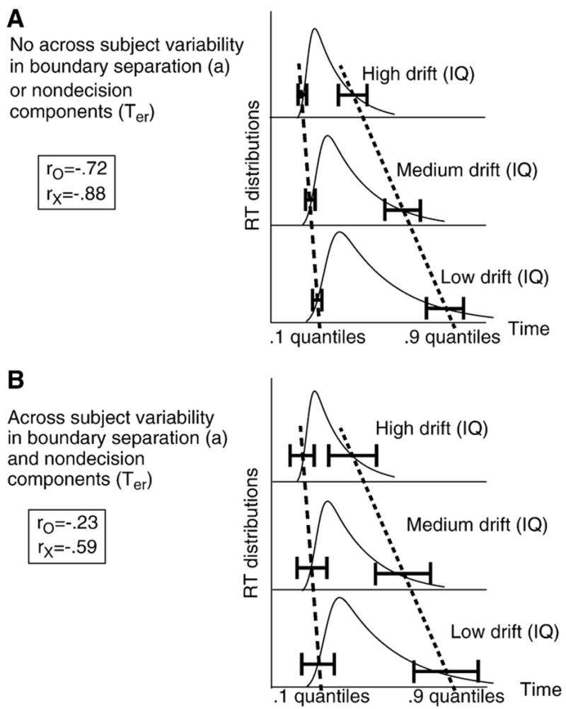
This illustrates how the worst performance rule could be obtained within the diffusion model framework. The two panels show RT distributions for three drift rates with horizontal error bars placed on the 0.1 and 0.9 quantile RTs. Panel A shows how the quantiles shift with decreasing drift rate, with relatively small error bars relative to the shift. Panel B shows that the error bars are much larger relative to the shift for the 0.1 quantiles than for the 0.9 quantiles when variability across subjects in boundary separation and the nondecision components of processing are added r_o represents the correlation of the .1 quantiles with drift rate and rx represents the correlations of the .9 quantiles with drift rate.

Panel A of Fig. 2 illustrates the situation with no across subject variability in boundary separation or the nondecision components of processing. Data simulated from the model do not conform to the worst performance rule (e.g., Table 1, row 1). The decrease from the high to the medium to the low drift rates is associated with increases in RTs and increases in each of the quantile values. Increases in the average 0.1 quantile from high to medium to low values of drift rate (the dashed line) relative to the variability in the quantiles, the horizontal bars, are a little smaller than for the average 0.9 quantile (the dotted line) relative to its variability in quantiles. This results in a slightly lower correlation between drift rate and the 0.1 quantile than between drift rate the 0.9 quantile; −0.72 and −0.88 respectively, for the simulated data in the first row of Table 1.

In Panel B, across subject variability in boundary separation and across subject variability the nondecision components are added. With these additions, data generated from the model do conform to the worst performance rule. The across subject variability in boundary separation and the nondecision components increase the variability in both the 0.1 and 0.9 quantiles for all levels of drift rate. The important point concerns how much variability is added to the quantiles relative to the shift in the quantiles across drift rates. The increase in variability in the 0.1 quantiles from Panel A to Panel B is a relatively large proportion of their Panel A variability, whereas the increase in variability in the 0.9 quantiles from Panel A to Panel B is a smaller proportion of their Panel A variability. This difference means that, in Panel B, the variability in the 0.1 quantiles is significantly larger relative to the shift in the 0.1 quantile across drift rates, while the variability in the 0.9 quantiles relative to their shift is much smaller. This is illustrated by the width of the horizontal bars and the lines through them; for the 0.1 quantiles, the bars for the high, medium, and low drift rates overlap vertically (the dashed line) while for the 0.9 quantiles, they do not (the dotted line). This means that the correlation between drift rate and quantiles is much lower for the 0.1 quantile than the 0.9 quantiles producing the worst performance rule (e.g., −0.23 and −0.59 for row 5 of Table 1).

To put it colloquially, adding variability in boundary separation and the nondecision components messes up the regularity in the shifts in the 0.1 quantiles (reducing the correlation), but because the shifts in the 0.9 quantiles are much larger, they are not messed up as much (and therefore reducing the correlation by less than for the 0.1 quantile).

3.1. Nondecision components of processing and the worst performance rule

The inspection time task has been used to study the effects of IQ on speed of processing (e.g., Deary, 2000; Grudnik & Kranzler, 2001; Kranzler & Jensen, 1989; Nettelbeck, 1987; Vickers & Smith, 1986). In this paradigm, two lines are displayed and then masked, and subjects have to decide which line is longer. The stimulus duration at some criterial level of accuracy is defined as inspection time. Findings that individual differences in performance on this task are related to intelligence suggest that IQ might correlated with the nondecision components of processing in the diffusion model. However, even if the duration of the nondecision components was correlated with IQ, then it alone does not produce the worst performance rule, in fact, it produces the opposite. This is because changes in T_er produces equal size shifts in all quantiles, thus, the shift in the 0.1 and 0.3 quantiles will be larger relative to their variability than the shift in the 0.7 and 0.9 quantiles relative to their variability. This results in the inverse of the worst performance rule (correlations decreasing from the 0.9 to the 0.1 quantiles) and a correlation of T_er with accuracy of zero.

4. Conclusions

The worst performance rule refers to the empirical finding that when IQ is correlated with RT, the correlation is larger for the slower than the faster responses. The simulations presented in this article show that the diffusion model predicts the worst performance rule if IQ is manifested in drift rate or if it is manifested in boundary separation. The key for the success of the model is variability in the values of components of processing across subjects. The simulations that demonstrated this result used values of the model parameters and values of variability across subjects in the parameters consistent with those from successful fits of the model to individual subject data (Ratcliff et al., 2001, 2003, 2004; Thapar et al., 2003). Furthermore, because the model also predicts accuracy, it demands that correlations be obtained between IQ and accuracy as well as RT quantiles. If IQ is manifested in drift rate, then the correlation between IQ and accuracy will be positive and the correlation between IQ and quantile RTs negative. If IQ is manifested in boundary separation, then both correlations will be negative with IQ (positive with boundary separation). This provides a way of discriminating between these two alternatives, but only because the diffusion model jointly accounts for RT and accuracy.

It should be stressed that there are patterns of parameter values for the diffusion model that would not produce the worst performance rule. For example, if IQ were not related to drift rate or boundary separation, but instead to the nondecision components of processing, the worst performance rule would not be observed. Also, it might be that other components of processing, such as across trial variability parameters vary across subjects in such a way that they correlate with IQ. For example, it might be that the higher the IQ, the lower the variability in drift rate. Hypotheses like these could be examined easily with simulations.

Schmiedek, Oberauer, Wilhelm, Süβ, and Wittmann (in press) linked the worst performance rule to RT distributions through an ex-Gaussian analysis (Luce, 1986; Ratcliff, 1979; Ratcliff & Murdock, 1976). For the ex-Gaussian, longer RTs are represented by an exponential parameter (τ), reflecting the tail of the RT distribution. Schmiedek et al. found that the estimates of τ for several RT tasks were strongly related to working memory and intelligence. Schmiedek et al. suggested that the diffusion model might provide a more parsimonious account of their findings than the usual explanation, that the worst performance rule arises from attentional lapses.

Other sequential sampling models (e.g., LaBerge, 1962; Ratcliff & Smith, 2004; Smith & Van Zandt, 2000; Smith & Vickers, 1988; Usher & McClelland, 2001) would likely produce similar results to those presented here. It would be relatively straightforward to simulate these models and check that the worst performance rule is obtained if IQ is assumed to be related to the rate at which information is accumulated or inversely related to decision boundary settings. However, this would be difficult because few of the models have been fit to data other than group data or to data from more than two or three individual subjects, partly because for some of the models, it can take upwards of 5 to 10 hours to adequately fit a single subject’s data.

In the framework of the diffusion model, the worst performance rule for RT quantiles as a function of drift rate or boundary separation is a natural consequence of across subject variability. To evaluate applications of the diffusion model, what is needed is first, to fit the model to data from real subjects individually, and second, to examine whether the values of the model parameters that best fit the data show the appropriate correlations between IQ and accuracy, mean RT, and RT quantiles.

References

- Baumeister AA, Kellas G. Distributions of reaction times of retardates and normals. American Journal of Mental Deficiency. 1968;72:715–718. [PubMed] [Google Scholar]
- Coyle TR. IQ, the worst performance rule, and Spearman’s law: A reanalysis and extension. Intelligence. 2003;31:567–587. [Google Scholar]
- Deary IJ. Looking down on human intelligence: From psychometrics to the brain. Oxford: Oxford University Press; 2000. [Google Scholar]
- Diascro MN, Brody N. Serial versus parallel processing in visual search tasks and IQ. Personality and Individual Differences. 1993;14:243–245. [Google Scholar]
- Grudnik JL, Kranzler JH. Meta-analysis of the relationship between intelligence and inspection time. Intelligence. 2001;29:523–535. [Google Scholar]
- Jensen AR. Reaction time and psychometric g. In: Eysenck HJ, editor. A model for intelligence. New York: Springer; 1982. pp. 93–132. [Google Scholar]
- Kranzler JH. A test of Larson and Alderton’s (1990) worst performance rule of reaction time variability. Personality and Individual Differences. 1992;13:255–261. [Google Scholar]
- Kranzler JH, Jensen AR. Inspection time and intelligence: A meta-analysis. Intelligence. 1989;13:329–347. [Google Scholar]
- LaBerge DA. A recruitment theory of simple behavior. Psychometrika. 1962;27:375–396. [Google Scholar]
- Larson GE, Alderton DL. Reaction time variability and intelligence: A “worst performance” analysis of individual differences. Intelligence. 1990;14:309–325. [Google Scholar]
- Luce RD. Response times. New York: Oxford University Press; 1986. [Google Scholar]
- Nettelbeck T. Inspection time and intelligence. In: Vernon PA, editor. Speed of information processing and intelligence. NJ: Ablex; 1987. pp. 295–346. [Google Scholar]
- Ratcliff R. A theory of memory retrieval. Psychological Review. 1978;85:59–108. [Google Scholar]
- Ratcliff R. Group reaction time distributions and an analysis of distribution statistics. Psychological Bulletin. 1979;86:446–461. [PubMed] [Google Scholar]
- Ratcliff R. A diffusion model account of reaction time and accuracy in a two choice brightness discrimination task: Fitting real data and failing to fit fake but plausible data. Psychonomic Bulletin and Review. 2002;9:278–291. doi: 10.3758/bf03196283. [DOI] [PubMed] [Google Scholar]
- Ratcliff R, Murdock BB., Jr Retrieval processes in recognition memory. Psychological Review. 1976;83:190–214. [Google Scholar]
- Ratcliff R, Rouder JN. Modeling response times for two-choice decisions. Psychological Science. 1998;9:347–356. [Google Scholar]
- Ratcliff R, Smith PL. A comparison of sequential sampling models for two-choice reaction time. Psychological Review. 2004;111:333–367. doi: 10.1037/0033-295X.111.2.333. [DOI] [PMC free article] [PubMed] [Google Scholar]
- Ratcliff R, Thapar A, Gomez P, McKoon G. A diffusion model analysis of the effects of aging in the lexical-decision task. Psychology and Aging. 2004;19:278–289. doi: 10.1037/0882-7974.19.2.278. [DOI] [PMC free article] [PubMed] [Google Scholar]
- Ratcliff R, Thapar A, McKoon G. The effects of aging on reaction time in a signal detection task. Psychology and Aging. 2001;16:323–341. [PubMed] [Google Scholar]
- Ratcliff R, Thapar A, McKoon G. A diffusion model analysis of the effects of aging on brightness discrimination. Perception & Psychophysics. 2003;65:523–535. doi: 10.3758/bf03194580. [DOI] [PMC free article] [PubMed] [Google Scholar]
- Ratcliff R, Thapar A, McKoon G. A diffusion model analysis of the effects of aging on recognition memory. Journal of Memory and Language. 2004;50:408–424. [Google Scholar]
- Ratcliff R, Tuerlinckx F. Estimating the parameters of the diffusion model: Approaches to dealing with contaminant reaction times and parameter variability. Psychonomic Bulletin and Review. 2002;9:438–481. doi: 10.3758/bf03196302. [DOI] [PMC free article] [PubMed] [Google Scholar]
- Ratcliff R, Van Zandt T, McKoon G. Connectionist and diffusion models of reaction time. Psychological Review. 1999;106:261–300. doi: 10.1037/0033-295x.106.2.261. [DOI] [PubMed] [Google Scholar]
- Salthouse TA. Relations of successive percentiles of reaction time distributions to cognitive variables and adult age. Intelligence. 1998;26:153–166. [Google Scholar]
- Schmiedek F, Oberauer K, Wilhelm O, Süβ H-M, Wittmann W. Individual differences in components of reaction time distributions and their relations to working memory and intelligence. Journal of Experimental Psychology:General. doi: 10.1037/0096-3445.136.3.414. in press. [DOI] [PubMed] [Google Scholar]
- Smith PL, Van Zandt T. Time-dependent Poisson counter models of response latency in simple judgment. British Lournal of Mathematical & Statistical Psychology. 2000;53:293–315. doi: 10.1348/000711000159349. [DOI] [PubMed] [Google Scholar]
- Smith PL, Vickers D. The accumulator model of two-choice discrimination. Journal of Mathematical Psychology. 1988;32:135–168. [Google Scholar]
- Thapar A, Ratcliff R, McKoon G. A diffusion model analysis of the effects of aging on letter discrimination. Psychology and Aging. 2003;18:415–429. doi: 10.1037/0882-7974.18.3.415. [DOI] [PMC free article] [PubMed] [Google Scholar]
- Usher M, McClelland JL. The time course of perceptual choice: The leaky, competing accumulator model. Psychological Review. 2001;108:550–592. doi: 10.1037/0033-295x.108.3.550. [DOI] [PubMed] [Google Scholar]
- Vickers D, Smith PL. The rationale for the inspection time index. Personality and Individual Differences. 1986;7:609–623. [Google Scholar]