Tomographic imaging of oxygen by phosphorescence lifetime

Abstract

Imaging of oxygen in tissue in three dimensions can be accomplished by using the phosphorescence quenching method in combination with diffuse optical tomography. We experimentally demonstrate the feasibility of tomographic imaging of oxygen by phosphorescence lifetime. Hypoxic phantoms were immersed in a cylinder with scattering solution equilibrated with air. The phantoms and the medium inside the cylinder contained near-infrared phosphorescent probe(s). Phosphorescence at multiple boundary sites was registered in the time domain at different delays (t_d) following the excitation pulse. The duration of the excitation pulse (t_p) was regulated to optimize the contrast in the images. The reconstructed integral intensity images, corresponding to delays t_d, were fitted exponentially to give the phosphorescence lifetime image, which was converted into the three-dimensional image of oxygen concentrations in the volume. The time-independent diffusion equation and the finite element method were used to model the light transport in the medium. The inverse problem was solved by the recursive maximum entropy method. We provide what we believe to be the first example of oxygen imaging in three dimensions using long-lived phosphorescent probes and establish the potential of these probes for diffuse optical tomography.

1. Introduction

Imaging tissue oxygen in vivo presents a challenging and important problem in modern physiology and medicine. Oxygen is an essential metabolite, and tissue hypoxia is a critical factor in many tissue pathologies, including retinal diseases,¹ brain abnormalities,^2,3 and cancer.^4,5 Imaging technologies suitable for mapping tissue oxygenation⁶ [e.g., nitroimidazole binding, NMR/EPR, positron emission tomography (PET), and near-infrared (NIR) tomographic techniques] range in their accuracy, invasiveness, and sensitivity, as well as in their temporal and spatial resolution. None, however, has have yet reached the stage of being a robust, generally accepted medical modality. The development of reliable quantitative methods for tomographic oxygen imaging is, therefore, very important.

One method that can directly quantify oxygen in tissue is based on the ability of oxygen to quench phosphorescence of exogenous probes.^7,8 When a phosphorescent probe is dissolved in a medium, its excited state lifetime and quantum yield become robust indicators of oxygen concentration. Phosphorescence quenching in solution is a diffusion-controlled process, which typically follows the linear Stern-Volmer relationship in the range of physiological oxygen concentrations:

$${\tau }_0∕\tau =I_0∕I=1+k_q\times {\tau }_0\times {\mathrm{pO}}_2,$$ (1)

where τ and I are the phosphorescence lifetime and integral intensity (quantum yield), τ₀ and I₀ are the phosphorescence lifetime and intensity in the absence of oxygen, pO₂ is partial oxygen pressure, and k_q is the bimolecular rate constant. This form of the Stern-Volmer equation assumes that oxygen in solution follows the Henry law, and the quenching constant k_q accounts for both the diffusion coefficient of oxygen in the immediate vicinity of the phosphorescent probe and oxygen solubility in the environment. Since the latter is typically unknown, it is useful to use the pressure rather that the concentration form of the Stern-Volmer equation.

The probability of collisional quenching by oxygen increases with an increase in the excited state lifetime, making longer decaying probes more sensitive to changes in oxygen concentration. Consequently, phosphorescent chromophores, characterized by long lifetimes (tens to hundreds of microseconds), are preferred over generally brighter but much faster decaying (nanoseconds) fluorescent chromophores. This is true despite the fact that from spin-statistical analysis the probability of fluorescence quenching by oxygen can be as much as nine times higher than the probability of phosphorescence quenching.⁹

The phosphorescence quenching method has been used to measure oxygen in a variety of biological objects, including the imaging of tissue hypoxia in two dimensions,¹⁰ and the feasibility of oxygen imaging through several centimeters of tissue has been demonstrated.¹¹ Recently, an array of long-lived NIR metalloporphyrin-based probes has been developed.¹² The quenching constants (k_q) of these probes can be tuned by dendritic encapsulation and their properties made insensitive to biological macromolecules by modifying the dendrimer periphery.^13,14 This new development has made it possible to consider combining the phosphorescence quenching method with NIR tomography to develop oxygen imaging in tissue in three dimensions. The first attempts to tomographically image oxygen by phosphorescence lifetime have recently appeared in the literature.^15-17

The theoretical foundation of phosphorescence lifetime imaging (PLI) closely resembles that of fluorescence lifetime imaging (FLI).^18-21 However, large differences between phosphorescent and fluorescent lifetimes (typically 4-5 orders of magnitude) bring about considerable differences in instrumentation and approaches to lifetime distribution reconstruction. For example, photon migration times in tissue are comparable to singlet state lifetimes of fluorescent contrast agents (nanoseconds). As a result, in FLI it is necessary to account for photon migration, whereas in PLI the propagation of excitation and emission can be considered instantaneous compared to triplet lifetimes (tens of microseconds). Consequently, forward and the inverse problems in PLI can be modeled in a much simpler way (see Subsections 2.A and 2.B).

Similarly, due to the long triplet lifetimes in PLI, the discrimination between background noise (e.g., endogenous fluorescence and backscattered excitation) and the signal of interest can be achieved by simple time gating. In FLI such filtering is impossible because the rates of photon emission and photon migration in the medium are comparable.

There has been a controversy in the literature regarding the use of long-lived luminescent probes in optical imaging. Some authors have argued that optical tomography with long-lived probes is generally not feasible because long triplet lifetimes cause uncertainty in the determination of the depths at which phosphorescent signals originate.^22,23 These investigators, however, did not take into account that lifetimes of phosphorescent probes change dramatically with physiological parameters of tissues (e.g., oxygenation). By introducing delays between excitation and acquisition, the contrast in the phosphorescent images of hypoxic objects can be effectively modulated and brought up to several hundreds. In a recent communication²⁴ we have computationally demonstrated that by using long-lived phosphorescent probes hypoxic inhomogeneities in scattering media could be imaged with good spatial accuracy. In the present paper we focus on the experimental imaging of hypoxic phantoms in a cylindrical model.

Previously, we used the telegraph equation to determine analytical solutions of the PLI forward problem for simple geometries.¹⁶ These solutions were used to solve the inverse problem in the frequency domain, and the validity of the method was confirmed by experimental reconstructions using a quasi-continuous wave (cw) setup in half-space geometry.¹⁷ However, our initial studies were limited to the simplistic case of zero-background phosphorescence, since carrying out spatial reconstructions using the quasi-cw method is impossible because of the strong influence of the background signal. To image true distributions of phosphorescence lifetimes, including the background phosphorescence, in this work we employ for the first time the time-domain approach, combining it with delayed integration and variable pulse length excitation (see Subsection 4.A infra). We use the quasi-steady-state diffusion equation to uncouple photon migration from phosphorescence and solve the forward problem numerically by the finite element method (FEM).²⁵ Further, we employ the maximum entropy method²⁶ (MEM) to solve the inverse problem formulated as a Fredholm integral equation of the first kind. The experiments presented demonstrate for what we believe to be the first time that oxygen distributions can be imaged quantitatively in scattering media in three dimensions using long-lived phosphorescent probes. The contrast in the images can be tuned by varying the width of the excitation pulses and delaying acquisition in the time domain. These experiments provide the basis for future development of in vivo oxygen tomography by phosphorescence lifetime.

We would like to mention that some parts of the image reconstruction scheme proposed here have been previously published, including in our earlier papers.^16,17 The present paper, however, presents the PLI tomographic methodology in its entirety, with some important elements that are significantly different from those in the previous studies.

2. Theory and Algorithms

The theoretical foundation of PLI closely resembles that of the absorption-scattering and fluorescent tomographies. A large body of literature covers these topics in great detail.^27-31 Here, we only summarize the main features of the underlying theory.

A. Forward Problem

The forward problem in PLI requires finding the distribution of the phosphorescence photon density in the medium given the position of the excitation source. The description of light propagation in the scattering media in the most general form is given bythe equation for radiation transport (ERT).³² The expansion of the ERT in spherical harmonics leads to the well-known diffusion approximation (p₁ approximation),^27,28 which has been widely used to model the forward problem in absorption-scattering³³ and fluorescent^15,19-21 tomography. Current research on photon migration models focuses on other approaches to ERT.^34-36 In this work we chose to use diffusion approximation as the simplest and best documented way to model light transport in tissue.

The coupled diffusion equations for the excitation photon density U^ex(r, t) and the emission photon density U^p(r, t) can be written in the following form:

$$\begin{array}{cc}\hfill & -\nabla k(\mathbf{r},{\lambda }_{\mathrm{ex}})\nabla U^{\mathrm{ex}}(\mathbf{r},t)+[{{\mu }_a}^t(\mathbf{r},{\lambda }_{\mathrm{ex}})+{{\mu }_a}^p(\mathbf{r},{\lambda }_{\mathrm{ex}})]\hfill \\ \hfill & \times U^{\mathrm{ex}}(\mathbf{r},t)+\frac{1}{c}\frac{\partial U^{\mathrm{ex}}(\mathbf{r},t)}{\partial t}=q_{\mathrm{ex}}(m_s,t),\hfill \\ \hfill & -\nabla k(\mathbf{r},{\lambda }_p)\nabla U^p(\mathbf{r},t)+{{\mu }_a}^t(\mathbf{r},{\lambda }_p)U^p(\mathbf{r},t)\hfill \\ \hfill & +\frac{1}{c}\frac{\partial U^p(\mathbf{r},t)}{\partial t}=q_p({\mathbf{r}}_s,t),\hfill \end{array}$$ (2)

where q_ex(m_s, t) represents the excitation sources located on the boundary, q_p(r_s, t) is the phosphorescence source located inside the medium (the subscript s denotes “source”), μ_a^t and μ_a^p are the absorption coefficients of the medium itself (e.g., tissue) and of the phosphorescent probe, respectively, k is the diffusion coefficient, and c is the speed of light. μ_a^t, μ_a^p, and k are functions of the wavelength λ, and they are bound by the following relationships:

$$\begin{array}{c}\hfill k(\mathbf{r},\lambda )=\frac{1}{3[{\mu }_a(\mathbf{r},\lambda )+{{\mu }_s}^{\prime }(\mathbf{r},\lambda )]},\hfill \\ \hfill {{\mu }_s}^{\prime }(\mathbf{r},\lambda )={\mu }_s(\mathbf{r},\lambda )(1-p_1),\hfill \end{array}$$ (3)

where μ_s(r, λ) is the scattering coefficient, μ_s’(r, λ) is the reduced scattering coefficient, and p₁ is the phase function.²⁸

The boundary conditions for the ERT specify that no photons can travel in the inward direction (from the outside into the medium) except for the photons originating on the boundary. For the diffusion approximation, the ERT boundary conditions are typically substituted by the Robin conditions²⁸:

$$U\left(m\right)+2k\left(m\right)A\frac{\partial U\left(m\right)}{\partial {\mathbf{n}}_0}=0,$$ (4)

where the constant A depends on the refraction parameter R: A = (1 + R)/(1 - R),²⁸ and n₀ is an outward normal vector to the boundary m.

For the time-domain case, the excitation sources q_ex(m_s, t) (Eq. 2) are typically approximated by point sources, positioned at the locations m_s of the boundary, firing at the moments t₀, and possessing infinitely short time constants:

$$q_{\mathrm{ex}}(m_s,t)=\delta (m-m_s)\delta (t-t_0).$$ (5)

Sources q_p(r_s, t) inside the medium [Eq. (2)] are represented by the functions of the probe absorption coefficient μ_a^p(r_s, λ_ex), the probe quantum yield ϕ₀ in the absence of oxygen,³⁷ the distribution of the excitation photon density U^ex(r_s, t), and the lifetime τ(r_s):

$$q_p({\mathbf{r}}_s,t)=U^{\mathrm{ex}}({\mathbf{r}}_s,t){{\mu }_a}^p({\mathbf{r}}_s,{\lambda }_{\mathrm{ex}}){\varphi }_0\delta (\mathbf{r}-{\mathbf{r}}_s)\exp \left[-\frac{t}{\tau \left({\mathbf{r}}_s\right)}\right].$$ (6)

The absorption coefficient μ_a^p(r_s, λ_ex) is the product of the probe concentration c(r_s) and the probe molar extinction coefficient ε(λ_ex). Here and throughout the text we assume that in the medium with constant oxygen concentration, phosphorescent probes decay single exponentially; however, multiexponential decays can also be considered by substituting for the exponential operator in Eq. (6) with an appropriate convolution integral.³⁸

It is necessary to account for all the excitation photons that arrive at the point r_s to initiate the luminescence decay. Although launched from the surface at exactly the same moment t₀ [Eq. (5)], these photons spread in time due to different diffusive pathways, which they encounter inside the volume. If the decay times are comparable to the times required for the photons to redistribute in the medium, photon migration will be convoluted with the decay kinetics. In PLI the decay rates are several orders of magnitude different from the photon migration rates, and that makes it possible to uncouple photon migration from photon emission. Thus Eqs. (2) can be separated, and the phosphorescence can be treated as if it is excited by an instantly switched on-off static field S^ex(r_s), the result of the integration of U^ex(r_s, t) in time:

$$S^{\mathrm{ex}}\left({\mathbf{r}}_s\right)=\int U^{\mathrm{ex}}({\mathbf{r}}_s,t)\mathrm{d}t.$$ (7)

Field S^ex(r_s), produced by a δ pulse [Eq. (5)], will be the same as the excitation photon density distribution U^ex(r) upon cw illumination. It will satisfy the steady-state diffusion equation

$$\begin{array}{cc}\hfill -& \nabla k(\mathbf{r},{\lambda }_{\mathrm{ex}})\nabla U^{\mathrm{ex}}\left(\mathbf{r}\right)+[{{\mu }_a}^t(\mathbf{r},{\lambda }_{\mathrm{ex}})+{{\mu }_a}^p(\mathbf{r},{\lambda }_{\mathrm{ex}})]U^{\mathrm{ex}}\left(\mathbf{r}\right)\hfill \\ \hfill & ={q_{\mathrm{ex}}}^{\prime }\left(m_s\right),\hfill \end{array}$$ (8)

where q_ex’(m_s) = δ(m - m_s) is a cw point source on the boundary.

On the other hand, the migration of phosphorescent photons also occurs much faster than phosphorescence emission; and the distribution of the phosphorescence photon density U^p(r) in each moment of time should also satisfy the steady-state approximation

$$-\nabla k(\mathbf{r},{\lambda }_p)\nabla U^p\left(\mathbf{r}\right)+{{\mu }_a}^p(\mathbf{r},{\lambda }_p)U^p\left(\mathbf{r}\right)=q_p\left({\mathbf{r}}_s\right),$$ (9)

where q_p(r_s) is a static phosphorescent source inside the medium. The evolution of a phosphorescent source in time is typically given by a single-exponential operator with the time constant τ(r_s), which is related to the local oxygen concentration through the Stern-Volmer relationship [Eq. (1)]. The decay of the source can be considered to be transmitted instantly to the entire volume by rapidly diffusing photons. Therefore the dependence of U^p(r_s) on time can be described by the same exponential operator exp[-t/τ(r_s)].

As a result, we arrive at the expression for the combined phosphorescence photon density, i.e., the probability of detecting a phosphorescence photon, produced by the excitation at a boundary point m_s (source) at time t₀, re-emitted as a point r inside the medium and detected at a point m_d (detector) also on the boundary:

$$\begin{array}{cc}\hfill U(\mathbf{r},m_s,m_d,t)=& \varphi \left(\mathbf{r}\right){{\mu }_a}^p(\mathbf{r},{\lambda }_{\mathrm{ex}})U^{\mathrm{ex}}(m_s,\mathbf{r})U^p(\mathbf{r},m_d)\hfill \\ \hfill & \times \exp \left[-\frac{t-t_0}{\tau \left(\mathbf{r}\right)}\right]\mathrm{d}\mathbf{r},\hfill \end{array}$$ (10)

where U^ex(m_s, r) and U^p(r, m_d) are the solutions of the steady-state Eqs. (8) and (9), respectively, for the excitation sources positioned at positions m_s and the detectors positioned at positions m_d.

For integrating detection devices, which can be rapidly turned on and off after a chosen delay time t_d (e.g., gated CCD cameras), the experimentally measurable boundary quantity M(m_d, t_d) is given by integral

$$M(m_d,t_d)=\frac{2}{A}{\int }_{t_d}^{\infty }\Gamma (m_d,t)\mathrm{d}t,$$ (11)

where

$$\Gamma (m_d,t)=\frac{1}{2}AU(m_d,t),$$ (12)

and A is the same as in boundary condition (4).²⁸

It should be mentioned that the same approximations are applicable to the frequency domain case of PLI. The dependence of the boundary phosphorescence amplitude and the phase shift on the modulation frequency will be merely a result of the Fourier transform applied to Eq. (10). It is also important that the distributions U^ex(m_s, r) and U^p (r, m_d) can be determined from models other than diffusion approximation and substituted into Eq. (10).

Analytical solutions of the photon diffusion equation can be established for a number of simple geometries.²⁷ However, numerical methods permit the treatment of arbitrary boundary geometries and absorption-scattering inhomogeneities. Following many researchers in the field,^39-41 in this work we applied the FEM²⁵ to model photon diffusion in the PLI forward problem.

B. Inverse Problem

In the most general form, the inverse problem in diffuse optical tomography can be formulated as a Fredholm integral equation of the first kind.⁴² For the frequency domain case of PLI the derivation of the integral equation has been published earlier.¹⁷ The same expression in the time domain can be written as

$$U(m_s,m_d,t)={\int }_{V}K(\mathbf{r},m_s,m_d)q^{\prime }[I_0\left(\mathbf{r}\right),\tau \left(\mathbf{r}\right),t]{\mathrm{d}}^3\mathbf{r},$$ (13)

where K is the transform kernel, which in the case of PLI is the product of the excitation and the phosphorescence photon density distributions Eq. (10):

$$K(\mathbf{r},m_s,m_d)=U^{\mathrm{ex}}(m_s,\mathbf{r})U^p(\mathbf{r},m_d).$$ (14)

The time evolution of the phosphorescence photon density distribution in the volume upon boundary δ excitation is given in Eq. (13) by the function q’[I₀(r), τ(r), t]:

$$\begin{array}{c}\hfill q^{\prime }[I_0\left(\mathbf{r}\right),\tau \left(\mathbf{r}\right),t]=I_0\left(\mathbf{r}\right)\exp \left[-\frac{t}{\tau \left(\mathbf{r}\right)}\right],\hfill \\ \hfill I_0\left(\mathbf{r}\right)={\varphi }_0{{\mu }_a}^p(\mathbf{r},{\lambda }_{\mathrm{ex}}),\hfill \end{array}$$ (15)

where τ(r) is related to the local oxygen concentration via the Stern-Volmer Eq. (1), I₀(r) is the initial intensity of the phosphorescence decay, and ϕ₀ and μ_a^p(r, λ_ex) are defined as in Eq. (6). It is the possibility of separating the spatial distribution of the phosphorescence (kernel K) from its evolution in time that is the key difference between the inverse problems of PLI and FLI. In the latter, photon migration affects the time dependence of the boundary signal and thus must be included explicitly in the expressions for U^ex(m_s, r) and U^p(r, m_d).

Combining Eqs. (13) and (11) we can write

$$\begin{array}{cc}\hfill M(m_s,m_d,t_d)& ={\int }_{V}K(\mathbf{r},m_s,m_d){\int }_{t_d}^{\infty }{q}^{\prime }[I_0\left(\mathbf{r}\right),\tau \left(\mathbf{r}\right),t]\hfill \\ \hfill & \times \mathrm{d}t{\mathrm{d}}^3\mathbf{r},\hfill \end{array}$$ (16)

and introducing the quantity

$$P(\mathbf{r},t_d)={\int }_{t_d}^{\infty }{I}_0\left(\mathbf{r}\right)\exp \left[-\frac{t}{\tau \left(\mathbf{r}\right)}\right]\mathrm{d}t=\tau \left(\mathbf{r}\right)I_0\left(\mathbf{r}\right)\exp \left[-\frac{t_d}{\tau \left(\mathbf{r}\right)}\right],$$ (17)

we obtain the final expression for boundary measurements:

$$M(m_s,m_d,t_d)={\int }_{V}K(\mathbf{r},m_s,m_d)P(\mathbf{r},t_d){\mathrm{d}}^3\mathbf{r},$$ (18)

where t_d is the start of the phosphorescence decay integration for the pair (m_s, m_d).

We assume that the phosphorescent probe is distributed homogeneously throughout the volume and that the scattering in the volume is uniform. This assumption, although not true for the majority of real systems, is a common initial guess for iterative reconstruction schemes. We collect data M(m_s, m_d, t_d) for several delay times t_d and compute the static kernel K after assigning some arbitrary starting values to μ_a^p and μ_s. Provided that a method of inversion of Eq. (18) exists, images P(r, t_d) can be reconstructed for each delay t_d. These images will represent the total numbers of photons emitted by the elements of the volume after each delay, and they can be fitted with a probe function g(r, t’),

$$g(\mathbf{r},t^{\prime })=c\times \tau \left(\mathbf{r}\right)\exp \left[-\frac{t^{\prime }}{\tau \left(\mathbf{r}\right)}\right],$$ (19)

to give the distribution of phosphorescence lifetimes τ(r). The constant c in Eq. (19) is related to the probe concentration and quantum yield. Thus performed, deconvolution provides a reasonable initial estimate for the image τ(r), which can be further refined by inverting Eq. (18) over the combined data set M(m_s, m_d, t_d) (for all delays t_d), using an appropriate positively constrained, regularized nonlinear inversion method.

The procedure outlined above will result in a true phosphorescence lifetime image τ(r) for uniformly absorbing and scattering media. All the experiments described below were limited to this case, and, therefore, we focus only on the method of inversion of Eq. (18) required for this particular type of analysis. A more general inversion method for nonhomogeneous distributions μ_a^p(r) and μ_s(r) will be addressed in future work. Such a method(s) will be similar to the inversion schemes employed in absorption-scattering tomography and in FLI, but with an important exception: In PLI, the recalculation of kernel K at each iteration is done in time-independent fashion, and this significantly reduces the computational cost of inversion.

We would also like to mention that a more common way to derive the inverse problem in diffuse optical tomography is via pertrubation theory.²⁸ Although formally different, this approach leads to essentially the same numerical optimization problem as does the formalism based on the Fredholm equation. Consequently, practical information, e.g., on the choice of regularization functionals,^43,44 can be interchanged between these approaches without modifying the main framework. Below in Subsection 2.C we follow the derivation based on the Fredholm integral equation and use the MEM²⁶ as a variant of the regularization technique.⁴⁵

C. Maximum Entropy Method

Because of the nature of kernel K the integral operator [Eq. (18)] that maps image P(r, t’) onto a data set M(m_s, m_d, t’) is highly ill-posed.⁴⁶ As a result, the exact inversion of Eq. (18) is impossible, and instead one seeks for an optimal image among the continuum of images that satisfies the data as required by an appropriate statistical functional, e.g. χ². According to Tikhonov’s regularization theory,⁴⁶ such an image corresponds to a constrained extremum of a regularization functional or regularizer. All practical inversion methods are different either by the choice of a nonlinear optimization scheme, designed to locate the constrained extremum, or by the regularizer itself. A special family of regularizers is formed by entropylike functionals⁴⁷ originating in the Shannon-Janes information theory.⁴⁸ The corresponding regularization method(s) are known as MEM.^49,50 MEM is usually described within the Bayesian framework,²⁶ and Bayesian reconstruction has been applied in diffuse optical tomography and in FLI in particular.^31,51

In an earlier work we developed a simple and compact recursive algorithm of the MEM⁵² and used it to analyze phosphorescence lifetime distributions in solutions¹³ and biological tissue.⁵³ In this paper the same recursive procedure was implemented for the inversion of Eq. (18). The description of the recursive MEM algorithm below largely follows that of Ref. 52.

After discretization, the inversion of Eq. (18) transforms into an inversion of a linear algebraic system. Using matrix notation and considering experimental noise η in the data this system can be written as

$$\mathbf{m}=\mathbf{Kp}+\eta$$ (20)

where m is an M-dimensional vector (M is the number of source-detector pairs) representing the data—phosphorescent decays integrated after delay t_d; p is an N-dimensional vector of unknown parameters, representing the image (N, the number of elements dividing the volume), and K is the design matrix—a discreet representation of the kernel K in Eq. (18). Matrix K consists of N M-dimensional vectors (rows) Kⁿ = K(p_n, x_i)(i = 1,...,M), where x_i represents the independent coordinate, i.e., a source-detector pair (m_s, m_d)_i. We define the probe function f(x) and the corresponding least-squares functional as

$$f\left(x\right)=\sum _n{p}_{n}K(p_n,x),$$ (21)

$${\chi }^2=\frac{1}{M}\sum _i\frac{1}{{{\sigma }_i}^2}{[f\left(x_i\right)-m_i]}^2,$$ (22)

where σ_i², is the noise variance for each datum m_i. Given the linear dependence of f(x) on parameters p, Eq. (22) can be rewritten as

$${\chi }^2=\frac{1}{2}\left(p,\mathrm{Hp}\right)-\left(g^o,p\right)+\sum _i\frac{{m_i}^2}{{{\sigma }_i}^2},$$ (23)

where H is the Hessian matrix and g^o is the antigradient vector calculated in the origin (p_n = 0, ∀n):

$$\begin{array}{c}\hfill {\mathrm{H}}_{mn}=\frac{2}{\mathrm{M}}\sum _i\frac{1}{{{\sigma }_i}^2}{K}^m\left(x_i\right)K^n\left(x_i\right)\hfill \\ \hfill {g_n}^{\mathrm{o}}=\frac{2}{\mathrm{M}}\sum _i\frac{1}{{{\sigma }_i}^2}{K}^n\left(x_i\right)m_i.\hfill \end{array}$$ (24)

The parentheses in Eq. (23) and in similar expression below denote scalar products.

The last term in Eq. (23) is a constant and does not affect optimizations. For convenience it will be omitted in the following expressions for χ². The minimization of χ² is equal to the maximization of Z = -χ²:

$$Z=\left(g^o,p\right)-\frac{1}{2}\left(p,\mathrm{Hp}\right),$$ (25)

which can be accomplished using an efficient and compact algorithm designed by Shrager.⁵⁴ Shrager’s algorithm assumes the nonnegativity constraints (p_n ≥ 0, ∀n), required by the physics of the problem. It converges in a finite number of steps and requires multiple inversions of submatrices derived from H. To assure numerical stability, the diagonal of H should be magnified. The magnification of the Hessian diagonal is, in fact, equivalent to adding a regularizer to the form Z (or -χ²). Using the Shannon-Janes entropylike functional S

$$S=-\sum _n{p}_n\ln \frac{p_n}{b_n}=-\left(p,l\right),$$ (26)

where b represents a priori knowledge about image p, and l denotes the vector with components l_n = ln(p_n/b_n), we introduce entropylike regularization into the maximization of Z. MEM searches for the maximum of S constrained by the data, i.e., χ² < ε for some small arbitrary value of ε. Usually ε is chosen to be 1 + 3.29/M^1/2.⁵⁰ The χ² constraints can be introduced into the search for the maximum of S using the Lagrange multiplier β, which gives functional Q:

$$Q=S-\beta {\chi }^2.$$ (27)

Using γ = 1/β and considering Eq. (25), we can restate the MEM problem as a maximization of Q’:

$$\begin{array}{cc}\hfill Q^{\prime }& =\gamma Q=-{\chi }^2+\gamma S=Z-\gamma \left(p,l\right)\hfill \\ \hfill & =\left(g^o,p\right)-\frac{1}{2}\left(p,\mathrm{Hp}\right)-\gamma \left(p,l\right)\hfill \\ \hfill & =\left(g^o,p\right)-\frac{1}{2}[\mathbf{p},(\mathbf{H}+\nu \Delta )\mathbf{p}],\hfill \end{array}$$ (28)

where ν = γ/2, and Δ denotes a diagonal matrix with elements

$$\begin{array}{c}\hfill {\Delta }_{nn}=\frac{\ln (p_n∕b_n)}{p_n},\hfill \\ \hfill {\Delta }_{mn}=0;m\ne n.\hfill \end{array}$$ (29)

A straightforward recursive procedure can be implemented for the maximization of Q’⁵²:

Step 0: Determine {σ_i} by analyzing noise η and compute matrix H and vector g^o.

Step 1: Choose ν and set the initial image p taking into account any available a priori information b; if information b is unavailable, set all parameters p to the same value.

Step 2: Magnify the diagonal of H using p [Eq. (29)] and use Shrager’s algorithm⁵⁴ to maximize Q’ and to produce a new image p_new.

Step 3: Set p = p_new and check if the convergence criterion is met; if yes—stop, if not, go back to Step 2.

The convergence is checked by the degree of anti-parallelism between the gradients of χ² and S, measured by the value of δ:

$$\delta =\frac{1}{2}\Vert \frac{\nabla {\chi }^2}{\Vert \nabla {\chi }^2\Vert }-\frac{\nabla S}{\Vert \nabla S\Vert }\Vert ,$$ (30)

where ∇χ² = Hp - g^o and ∇S = -l. A true maximum entropy solution is achieved when δ is zero. Normally, convergence with δ < 10^-4 is reached after approximately ten iterations.

In our algorithm we make use of the so-called active set approach.⁵⁵ As MEM converges, the elements of the image with values approaching zero are excluded from the search space. Thus the dimensions are reduced and convergence accelerated. Consequently, images of small objects with a zero background are computed faster than images with many nonzero pixels. Nevertheless, the full size Hessian matrix H is inverted at least once in the beginning, and this largely defines the computational speed of the procedure.

Two issues must be worked out before the algorithm is applied to experimental image reconstruction: (1) the value of the magnification parameter ν, and (2) the procedure for the inversion of H. It has been shown that the value of ν is dependent on the noise in the data,⁵² which is consistent with the regularization theory.⁴⁶ By doing numerical simulations, this dependence can be elucidated and embedded into the automatic search routine.

Since H is a positive-definite symmetrical matrix, the Cholesky algorithm⁵⁶ is the most appropriate for its decomposition. However, when the number of nodes in the volume is large (5000 or more) even the Cholesky routine becomes computationally expensive. In that case, a stepwise procedure can be adopted, in which the volume is first divided by a crude mesh, and the regions with nonzero phosphorescence identified. The obtained low-resolution image is then refined, using the crude reconstruction as a priori information b [Eqs. (26) and (29)]. It should be mentioned that the algorithm described above was originally designed with small-scale problems (N < 1000) in mind. In cases in which the number of nonzero pixels in the image is large other algorithms, e.g., the classic procedure of Skilling and Bryan,⁵⁰ should be more efficient.

3. Materials and Methods

All programs were written in C/C++ and run on a single processor 2.5 GHz personal computer (PC) with 2 Gb in core storage capacity. The main components of the code were the FEM-based forward problem solver, the simulator of boundary data, and the MEM-based inverse problem solver. The design matrices and Hessians corresponding to different values of μ_s’ and μ_a (optically homogeneous media), different grid resolutions, and different numbers and positions of source-detector pairs could be precomputed and stored on the disk for simulations.

The imaging experiments were performed using an in-house constructed single-detector phosphorometer—a time-domain variant of an earlier described frequency-domain system.⁵⁷ The phosphorometer was built around a 333 kHz 16-bit board (National Instruments, MIO-6059). The detector was an APD (Hamamatsu, 3 μs rise time), and the excitation source was an LED (Luxeon Star III, 3 W, λ_max = 635 nm). Separate power supplies were used for the APD and the LED to avoid cross talk between the devices. The excitation and the emission were conducted from and to the instrument by 3 mm glass light guides. The emission was filtered through a long-pass (695 nm cutoff) filter and focused on the APD surface by a spherical lens. The phosphorescence decays were recorded during a 3 ms time period.

Two phosphorescent dyes were used in our experiments: Oxyphor G2 [Fig. 1(a)]^14,58 and Oxyphor G3 [Fig. 1(b)].⁵⁹

Fig. 1.

Phosphorescent probes (a) Oxyphor G2, (b) Oxyphor G3, and (c) their absorption and emission spectra.

Pd tetrabenzoporphyrin-dendrimers G2 and G3 differ by the dendrimer composition (G2, polyglutamate; G3, polyarylglycine) and surface coatings (G2, none; G3, PEG, average molecular weight (MW) 350). G2 (MW 2,642) is designed to be used in combination with albumin, which provides additional coating for the phosphor; whereas G3 (MW 16,100) does not interact with albumin due to the surface layer of oligo-ethyleneglycols (PEGs). Its dendritic environment (arylglycine dendrons) folds tightly around the core in aqueous media and controls the accessibility of oxygen to the porphyrin. The absorption and the phosphorescence spectra of G2 and G3 are nearly identical [Fig. 1(c)]. Both phosphors are characterized by quantum yields of approximately 7%-10% and lifetimes τ₀ of approximately 180 μs for Oxyphor G2 and 280 μs for Oxyphor G3 in deoxygenated aqueous solutions. Oxygen quenching constants (k_q) of G2 and G3 in water at 23 °C are 1,800 mm Hg^-1 s^-1 and 110 mm Hg^-1 s^-1, respectively. These values translate into lifetimes of <5 μs (G2) and 45 μs (G3) at ambient air pressures (pO₂ ≈ 151 mm Hg).

The scattering medium was prepared using Intralipid (Sigma). The intralipid and india ink were added to the solution of the phosphorescent probe to give optical properties, close to those of some biological tissue: μ_a^p = 0.008 mm^-1, μ_s’ = 0.5 mm^-1 (Ref. ⁶⁰). The resulting solution was placed in a Naglene cylindrical vial (Ø 6 cm, h = 10 cm). Hypoxic phantoms were emulated by Naglene capsules. Solutions within the capsules were deoxygenated by bubbling with purified argon, and then the capsules were sealed. The cylinder with the immersed hypoxic phantoms was placed inside a thick-walled cylindrical holder with holes allowing access of light guides. The imaging experiment was conducted by stepwise collection of all the decays corresponding to source-detector pairs by a manual positioning of the light guides.

4. Results and Discussion

The discussion in this section focuses on the contrast in phosphorescence lifetime images, on numerical simulations, and on an experimental demonstration of the developed approach.

A. Lifetime-Based Contrast in Luminescence Enhanced Imaging

Photon migration in scattering media occurs on the same time scale (nanoseconds) as does singlet state emission (fluorescence). The shorter the lifetime of a fluorescent probe and the less scattering occurs in the medium, the more resolved in time are the signals corresponding to the objects positioned at different depths in the volume. In a hypothetical case, when the probe’s excited-state lifetime is zero (i.e., instantaneous emission) and in the absence of scattering, objects can be located by simply measuring the time delay between the excitation and emitted light—an “echo”-type experiment. Scattering alters the trajectories of photons and broadens the photon wave in time. Uncertainty in the time of emission, associated with the time that the probe spends in its excited state, introduces additional broadening, making discrimination between photons emitted at different depths in the volume increasingly difficult. Nevertheless, when the lifetime of the probe is comparable to the photon migration time (fluorescent probe), it is possible to correlate the kinetics of the signal with the depth(s) at which the emission originated. In an earlier study²² the feasibility of imaging with long-lived phosphorescent probes was challenged on the grounds that phosphorescent lifetimes, which are much longer than photon migration times, do not permit a correlation of the signal kinetics with the probability of emission being generated at a particular depth. This conclusion, however, is not relevant to the mechanism of lifetime-based contrast enhancement occurring in PLI. Triplet lifetimes (tens to hundreds of microseconds) are orders of magnitude longer than photon migration times, even if photons travel deep into tissue (tens of centimeters). Consequently, the emission of phosphorescence should be regarded as a quasi-static process with respect to the photon migration time scale.

However, it is the alterations in phosphorescence lifetimes due to their high sensitivity to oxygen in the environment that make them an extremely effective tool for contrast enhancement. In a recent paper²⁴ we demonstrated how a delayed acquisition in the time domain can enhance the contrast between short-lived phosphorescence of normoxic background and long-lived phosphorescence of hypoxic objects, even when the phosphorescent probe is distributed uniformly in the medium and not confined to the regions of hypoxia. The introduction of a delay t_d between the excitation pulse and the start of the data acquisition in the time domain leads to an increase in the fraction of the long-lived component in the overall signal. For two volumes characterized by phosphorescence lifetimes τ₁ and τ₂ [τ₂ > τ₁,pO₂(2) < pO₂(1)] and absorbing the same number of excitation photons, the ratio C(t_d) of integral intensities, corresponding to these equal volumes, increases with delay t_d as

$$C\left(t_d\right)=\frac{{\tau }_2}{{\tau }_1}\exp \left(\frac{{\tau }_2-{\tau }_1}{{\tau }_1{\tau }_2}{t}_d\right).$$ (31)

The longer the delay t_d, the lesser fraction of the short-lived signal is present in the data, the higher the contrast in the images. By numerical simulations we have shown²⁴ that for typical oxygen concentrations and existing phosphorescent probes signal-to-noise ratios (SNRs) obtained after removing the initial “fast” parts of phosphorescent decays are still adequate for accurate image reconstructions. Nevertheless, increasing the SNRs while keeping high contrast is highly desirable, and can be accomplished by extending the length of the excitation pulses.

The phosphorescent response of a single-exponential source to the excitation in the form L(t’) is given by the convolution integral:

$$I\left(t\right)={\int }_{\mathrm{o}}^{t}L\left(t^{\prime }\right)I_0\exp \left(-\frac{t-t^{\prime }}{\tau }\right)\mathrm{d}{t}^{\prime },$$ (32)

where I₀ is proportional to the probe absorption coefficient and the phosphorescence quantum yield, as in Eq. (19). For two volumes with lifetimes τ₁ and τ₂ (τ₂ > τ₁), equally excited by a rectangular pulse of duration t_p, the ratio R(t_p) of the phosphorescence intensities by the end of the pulse will be

$$R\left(t_p\right)=\frac{{\tau }_2\left[1-\exp \left(-\frac{t_p}{{\tau }_2}\right)\right]}{{\tau }_1\left[1-\exp \left(-\frac{t_p}{{\tau }_1}\right)\right]}.$$ (33)

Upon an increase in the duration of the pulse (t_p → ∞, steady-state excitation), R(t_p) will asymptotically approach the ratio of the phosphorescence lifetimes τ₂/τ₁, whereas at short t_p’s (t_p → 0, δ pulse) the phosphorescence intensities of both components (τ₁ and τ₂) will be nearly equal. Therefore by increasing the duration of the pulse one can increase the initial intensities of decays with longer lifetimes (hypoxic objects) relative to those with shorter lifetimes (normoxic background). Importantly, the SNRs of the overall decays will not change as long as the integral intensities of the excitation pulses remain the same; for pulses with constant peak intensities, typical for conventional light sources, longer t_p’s will not only improve the contrast but will also increase the SNRs simultaneously.

The combined contrast ratio κ, achieved by both increasing the pulse width t_p and introducing delay t_d, will be the product of C(t_d) and R(t_p):

$$\kappa (t_p,t_d)=R\left(t_p\right)C\left(t_d\right).$$ (34)

The dependence of κ on pulse duration t_p for two equally excited volumes at different delay times t_d is shown in Fig. 2. We demonstrate in Subsections 4.B and 4.C how by changing delays t_p and t_d the contrast in images of differently oxygenated volumes can be regulated.

Fig. 2.

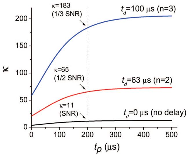
(Color online) Simulation of dependence of contrast ratio κ on pulse duration t_p for different delays t_d. Two volumes with pO₂(1) = 50 mm Hg^-1 (τ₁ = 25 μs) and pO₂(2) = 10 mm Hg^-1 (τ₂ = 91 μs), containing equal amounts of phosphorescent probe (k_q = 700 mm Hg^-1 s^-1, τ₀ = 250 μs), were equally excited by a rectangular pulse of duration t_p. Delays t_d (start of the data integration) correspond to the moments of time when the intensity of the decay with longer lifetime (τ₂) was reduced n times: t_d(n) = τ₂ ln(n).

B. Numerical Simulations

An accurate solution of the forward problem is the key to successful image reconstruction. In our program we used a FEM-based solver to model photon diffusion in cylindrical objects. The solver was tested for numerical stability and consistency, i.e., the ability to reproduce an exact solution of the differential Eqs. (8) and (9) upon refinement of the mesh.

The main component of our image reconstruction scheme is the MEM algorithm, based on recursions of the quadratic optimization routine.⁵⁴ This algorithm has been tested previously⁵² for its ability to restore images maximally close to the original at high SNRs, while introducing reasonable blurring upon an increase in the level of noise. Critical to the performance of the algorithm is the choice of regularization parameter ν, Eq. (28). Parameter ν weights the solution toward the unconstrained maximum of entropy S [Eq. (26)] at high levels of noise (less detailed image) and brings it closer to the positively constrained minimum of χ² [Eq. (23)] at higher SNRs. By doing simulations using different images and different noise levels we elucidated the empirical dependence of ν on the level of noise in the data.

Here and throughout the text we define the SNR of a phosphorescent decay as the ratio of the intensity in the beginning of the decay (e.g. the counts in the first channel) to the mean-square amplitude (σ²) of the noise. Thus two decays with equal initial intensities but different lifetimes have the same SNRs. Upon introduction of delay t_d [Eq. (31)] and, consequently, removing some part of the decay, the SNR of the decay will decrease. We define the SNR of a data set (i.e., a set of decays for all source-detector pairs) as the SNR of the decay with maximal initial intensity. In the experiments described below, a light source with constant peak intensity was used. Therefore an increase in the pulse duration (t_p) led to an increase in the SNR. Typically, for t_p = 100 μs, SNRs of approximately 200-300 were obtained.

An example of a typical numerical experiment used to test the performance of the system is depicted in Fig. 3. Two deoxygenated elliptical objects (d_xy = 12 mm, d_z = 20 mm) were positioned inside a cylinder (Ø 60 mm, d_z = 100 mm) as shown in Fig. 3(a). The parameters of the medium were chosen to be μ_a (635 nm) = 6 × 10^-3 mm^-1, μ_a (810 nm) = 2.8 × 10^-4 cm^-1, and μ_s’ (635 nm) = 0.5 mm^-1, μ_s’ (810 nm) = 0.4 mm^-1. The phosphorescence lifetimes were 180 and 280 μs for the capsules and 30 μs for the background (Fig. 3). The entry points for the source-detector light guides (24 in total) were positioned on the periphery of the cylinder in hexagonal fashion on four levels, giving the total of 552 source-detector pairs. For simulations, the volume inside the cylinder was divided into 90,450 triangular prisms with an average linear size of 1.7 mm. The boundary data were simulated by summing up all the decays originating in the grid elements (phosphorescent sources). The lifetimes of the individual sources were calculated based on the prechosen oxygen distribution, whereas their initial intensities were found from the solution of Eq. (10) for each source-detector pair. For rectangular excitation pulses (t_p ≠ 0), the initial intensities were weighted according to Eq. (33). Normally distributed noise with constant amplitude was added to all the decays in the data set to produce the desired SNR. In total, 900 data points (3.3 μs per point) were recorded per decay. The data set was scaled to match the response of a 16-bit analog-to-digital converter and integrated at delay times t_d [see Eq. (11)] to give a series of input arrays for subsequent MEM analyses. The design matrix for the MEM was based on the same FEM solution used in the simulations, but it was spanned over a cubic mesh with 2,980 elements (d_xyz = 4.6 mm). The data arrays were inverted to give a series of intensity images P(t_d) [see Eq. (18)], which were fitted by single exponentials in every point of the spatial grid to give the phosphorescence lifetime image.

Fig. 3.

(Color online) Numerical simulation and recovery of phosphorescence lifetime distributions in the scattering cylinder (dimensions in millimeters). Dots on the periphery of the cylinder correspond to the positions of the source and detector sites. Only cross sections (x-z plane) of complete 3D images are shown. (a) Integral intensity images recovered by the MEM from the data obtained at different delays t_d (shown above the images in microseconds). Data set (a) was produced using a 70 μs excitation pulse (t_p = 70 μs), SNR = 135. Lifetime images (b) and (c) were obtained by fitting the intensity images either (b) including all the images in the series, t_d = 13-472 μs, or (c) ignoring the images taken at shorter delays t_d = 36-472 μs. The lifetime scale (microseconds) is shown on the left in pseudocolor. Images (b) and (c) were produced using excitation pulses of different lengths (t_p = 10, 70, and 250 μs).

Lifetime images, produced by fitting sets of intensity images, such as the one shown in Fig. 3(a) (t_p = 70 μs), are presented in Figs. 3(b) and (c). Only the x-z cross sections of the complete 3D images are shown. Other cross sections revealed equally good correspondence with the model. The integral intensity maps [P(t_d)] recovered by the MEM [Fig. 3(a)] show how the phosphorescence from the normoxic background (τ = 30 μs) decays rapidly, while the hypoxic capsules, especially the one with the longer lifetime τ = 280 μs, continue to glow throughout the entire series.

The effects of contrast enhancement by increasing either the acquisition delay (t_d) or the pulse length (t_p), or both, are particularly evident in the lifetime images in Figs. 3(b) and (c). Two sets of images, obtained by fitting the whole series [Fig. 3(b) t_d = 13-472 μs] or leaving out the first delay [Fig. 3(c) t_d = 36-472 μs] are shown. Because the short-lived signal (τ = 30 μs) has already decayed considerably at t_d = 36 μs, only a fraction of the background phosphorescence appears in the images in Fig. 3(c). By contrast, when the first intensity image (t_d = 13 μs) is included in the fitting [Fig. 3(b)] the signal from the background is seen quite well. Indeed, at 13 μs the exponent with τ = 30 μs decayed down only to approximately 65% of its initial intensity.

The contrast in the lifetime images is further amplified by increasing the length of the excitation pulse t_p [Eq. (33)]. This effect makes it possible to suppress the initial intensities of short-lived phosphorescent signals. In both series of images [Figs. 3(b) and (c)] the background gradually disappears with the pulse length increasing from 10 to 250 μs. In the last image in Fig. 3(c) (t_p = 250 μs, t_d = 36 μs), the combined contrast κ [see Eq. (34)] between the longer lifetime (τ = 280 μs) and the background (τ = 30 μs) reaches as high as 150 (after normalization for the excitation density), which results in a complete elimination of the background and brightens the images of the hypoxic capsules.

The simplistic procedure used to obtain lifetime images obviously suffers from a number of deficiencies. For example, it tends to reduce the peak lifetimes in the hypoxic regions, while increasing the lifetimes in the nearby background. This mixing effect can be rationalized considering that lifetime images were obtained by the exponential fitting of intensity images, individually recovered by the MEM. For the same object, MEM-recovered images at lower SNRs (longer delays t_d) are broader than those at high SNRs (shorter delays t_d). Consequently, if the object’s true peak intensity decays as exp(-t_d/τ), the peak intensities of MEM-recovered images will decay with a faster rate, exp(-t_d/τ) - Δ_d, where Δ_d is an extra decrease in intensity due to the MEM-induced broadening. Δ_d increases with an increase in t_d (lower SNR, broader image, lower peak intensity), and consequently the fitting will result in a faster apparent rate of decay and shorter apparent lifetime τ - δτ. At the same time, the leak of phosphorescence into the surrounding background will increase the apparent lifetime of the latter. This and other deficiencies of the procedure can be corrected in the following refinement of the lifetime image. The refinement will involve fitting the data sets for all delays t_d simultaneously, varying the distributions of τ as well as the scattering and absorption coefficients μ_a and μ_s’ to account for the optical heterogeneity of the medium.

C. Experimental Image Reconstructions

To check the applicability of the approach to real experimental systems we performed several test experiments on inhomogenously oxygenated hypoxic phantoms. The purposes of these experiments were to evaluate whether SNR levels permit phosphorescence lifetime-oxygen distribution reconstruction in real systems; to determine whether the presence of background phosphorescence allows the imaging of hidden hypoxic phantoms; and to determine whether phosphorescence lifetimes can be determined quantitatively in 3D. Although our software was designed for future use with integrating detectors (e.g., CCD cameras), in the experiments described here we used a simple time-resolved phosphorometer, previously designed to measure lifetime distributions in heterogeneous samples.⁵⁷ The profile of the excitation pulse in this instrument was software controlled, and therefore it was simple to change the operation of the instrument from time to frequency domain. Phosphorescence decays collected by the instrument could be integrated at all desirable delays t_d.

Two experimental image reconstructions are shown in Fig. 4. In both cases the deoxygenated phantom was a tube (Ø 12 mm) positioned inside a cylinder (Ø 6 cm) at an angle relative to the cylinder’s z axis. In the first experiment [images Figs. 4(a) and 4(b) and the corresponding intensity images Fig. 4(e)] the solution contained Oxyphor G2 (see Subsection 4.C), whose phosphorescence at ambient oxygen pressure was significantly quenched (τ₁ < 5 μs). In the second, both the background solution and the solution inside the capsule contained Oxyphor G3, whose lifetime at air saturation at ambient temperature is τ₁ = 45 μs.

Fig. 4.

(Color online) Experimental image reconstructions in a cylinder. x-z cross sections of complete 3D images are shown (dimensions in millimeters). Excitation pulse was 200 μs long (t_p = 200 μs). (a) Oxygen image and (b) phosphorescence lifetime image of a phantom (τ₂ = 190 μs, pO₂ = 0.2 Torr, Oxyphor G2) in solution with a low background (τ₁ < 5 μs). Lifetime image was recovered using a series of MEM-reconstructed phosphorescence intensity images (e), with the first image (not shown in the figure) taken after a delay t_d¹ = 27 μs. (c) and (d) Lifetime images of the phantom (τ₂ = 170 μs) in solution with strong background phosphorescence ( τ₁ = 45 μs, Oxyphor G3). Lifetime image obtained from intensity images taken after delays (c) t_d¹ = 20 μs and (d) t_d¹ = 60 μs.

It is clear that in both cases the positions and the lifetimes of the phantoms were reconstructed with good accuracy. In the case with the low background [Figs. 4(a) and 4(b); τ₁ < 5 μs], very high contrast could be achieved practically without jeopardizing the phosphorescence signal (t_d¹ = 27 μs), especially using long excitation pulses (t_p = 200 μs). The SNR of the data set for this pulse length and delay was 132. The resulting oxygen image [Fig. 4(a)] appears quite uniform with an average oxygen pO₂ of approximately 0.3 mm Hg^-1 s^-1, which is only slightly higher than that in the original solution.

The lifetime images obtained in the case of the phantom with τ₂ = 170 μs, placed in the medium with strong residual phosphorescence (τ₁ = 45 μs), also reveal the position of the phantom quite well. However, even when relatively long excitation pulses were used (t_p = 200 μs), the residual background was still present in the image [Fig. 4(c)] at short acquisition delays (t_d¹ = 20 μs, SNR = 136). Removing the background was possible by rejecting the initial part of the decays [Fig. 4(d), t_d¹ = 60 μs]. In this case, the SNR of the data set was reduced to 79; however, the actual signal from the hypoxic capsule, most relevant to the recovery, was still 73% of its initial value. As a result, the reconstruction of the position of the capsule was achieved with good accuracy, whereas the background was nearly fully eliminated.

The experiments presented in Fig. 4 show that probes with high k_q’s (e.g., Oxyphor G2 in the absence of albumin) produce almost no phosphorescent signal unless the pO₂ in the system drops down to extremely low values (pO₂ ≈ 0). Such probes can be useful for detection of regions only of very severe hypoxia. At the same time, probes with moderate-to-low k_q’s (e.g., Oxyphor G3) exhibit phosphorescence at all oxygen concentrations throughout the physiological range, but offer lower intrinsic contrast. An optimal range of quenching constants can be determined for each particular imaging application, although probes with quenching constants of 500-700 mm Hg^-1 s^-1 are perhaps the most effective for detecting regions of tissue hypoxia, providing both sufficient contrast and sensitivity.

5. Conclusions

In this paper we present, for what we believe is the first time, a complete method for the tomographic imaging of absolute oxygen concentrations in turbid media in three dimensions using long-lived phosphorescent probes. The feasibility of tomographic phosphorescence lifetime imaging (PLI) is demonstrated by both numerical simulations and experimentally, using cylindrical models as examples. The key features of the proposed approach are as follows:

1. The forward problem in PLI can be solved in time-independent fashion, given the large differences between the photon migration times and the times of phosphorescence emission.

2. The inverse problem in PLI in the first approximation can be solved by reconstructing a series of phosphorescence intensity images, taken at different delays after the excitation pulse in the time domain, and fitting these images with exponentials in every element of the spatial grid; the maximum entropy method can be applied effectively for image reconstruction.

3. The contrast between the areas of different oxygenation can be enhanced by (a) introducing a delay between the excitation pulse and the beginning of data acquisition in the time domain and (b) modifying the duration of the excitation pulse.

4. Delayed data acquisition allows a complete removal of the noise resulting from scattered excitation light and endogenous fluorescence.

The future development of oxygen tomography and PLI will include the development of efficient algorithms for inverse problems and the construction of appropriate multichannel imaging instrumentation.

References and Notes

- 1.Arden GB, Sidman RL, Arap W, Schlingemann RO. Spare the rod and spoil the eye. Br. J. Ophthamol. 2005;89:764–769. doi: 10.1136/bjo.2004.062547. [DOI] [PMC free article] [PubMed] [Google Scholar]
- 2.Pena F, Ramirez AM. Hypoxia-induced changes in neuronal network properties. Mol. Neurobiol. 2005;32:251–283. doi: 10.1385/MN:32:3:251. [DOI] [PubMed] [Google Scholar]
- 3.Ferriero DM. Medical progress—neonatal brain injury. New Eng. J. Med. 2004;351:1985–1995. doi: 10.1056/NEJMra041996. [DOI] [PubMed] [Google Scholar]
- 4.Evans SM, Koch CJ. Prognostic significance of tumor oxygenation in humans. Cancer Lett. 2003;195:1–16. doi: 10.1016/s0304-3835(03)00012-0. [DOI] [PubMed] [Google Scholar]
- 5.Shah N, Cerussi AE, Jakubowski D, Hsiang D, Butler J, Tromberg BJ. The role of diffuse optical spectroscopy in the clinical management of breast cancer. Dis. Markers. 2003;19:95–105. doi: 10.1155/2004/460797. [DOI] [PMC free article] [PubMed] [Google Scholar]
- 6.Ballinger JR. Imaging hypoxia in tumors. Semin. Nucl. Med. 2001;31:321–329. doi: 10.1053/snuc.2001.26191. [DOI] [PubMed] [Google Scholar]
- 7.Vanderkooi JM, Maniara G, Green TJ, Wilson DF. An optical method for measurement of dioxygen concentration based on quenching of phosphorescence. J. Biol. Chem. 1987;262:5476–5482. [PubMed] [Google Scholar]
- 8.Wilson DF, Vinogradov SA. Tissue oxygen measurements using phosphorescence quenching. In: Mycek M-A, Pogue BW, editors. Handbook of Biomedical Fluorescence. Marcel Dekker; 2003. pp. 637–662. [Google Scholar]
- 9.Saltiel J, Atwater BW. Spin-statistical factors in diffusion controlled reactions. In: Volman DH, Hammond GS, Gollnick K, editors. Advances in Photochemistry. Wiley; 1988. pp. 1–90. [Google Scholar]
- 10.Rumsey WL, Vanderkooi JM, Wilson DF. Imaging of phosphorescence: a novel method for measuring the distribution of oxygen in perfused tissue. Science. 1988;241:1649–1651. doi: 10.1126/science.241.4873.1649. [DOI] [PubMed] [Google Scholar]
- 11.Vinogradov SA, Lo L-W, Jenkins WT, Evans SM, Koch C, Wilson DF. Noninvasive imaging of the distribution of oxygen in tissue in vivo using near-infrared phosphors. Biophys. J. 1996;70:1609–1617. doi: 10.1016/S0006-3495(96)79764-3. [DOI] [PMC free article] [PubMed] [Google Scholar]
- 12.Finikova OS, Cheprakov AV, Vinogradov SA. Synthesis and luminescence of soluble meso-unsubstituted tetrabenzo- and tetranaphtho[2,3]porphyrins. J. Org. Chem. 2005;70:9562–9572. doi: 10.1021/jo051580r. and references therein. [DOI] [PMC free article] [PubMed] [Google Scholar]
- 13.Rozhkov VV, Wilson DF, Vinogradov SA. Phosphorescent Pd porphyrin-dendrimers: tuning core accessibility by varying the hydrophobicity of the dendritic matrix. Macromolecules. 2002;35:1991–1993. [Google Scholar]
- 14.Rietveld IB, Kim E, Vinogradov SA. Dendrimers with tetrabenzoporphyrin cores: near-infrared phosphors for in vivo oxygen imaging. Tetrahedron. 2003;59:3821–3831. [Google Scholar]
- 15.Shives E, Xu Y, Jiang H. Fluorescence lifetime tomography of turbid media based on an oxygen-sensitive dye. Opt. Express. 2002;10:1557–1562. doi: 10.1364/oe.10.001557. [DOI] [PubMed] [Google Scholar]
- 16.Soloviev VY, Wilson DF, Vinogradov SA. Phosphorescence lifetime imaging in turbid media: the forward problem. Appl. Opt. 2003;42:113–123. doi: 10.1364/ao.42.000113. [DOI] [PubMed] [Google Scholar]
- 17.Soloviev VY, Wilson DF, Vinogradov SA. Phosphorescence lifetime imaging in turbid media: the inverse problem and experimental image reconstruction. Appl. Opt. 2004;43:564–574. doi: 10.1364/ao.43.000564. [DOI] [PubMed] [Google Scholar]
- 18.Patterson MS, Pogue BW. Mathematical model for time-resolved and frequency-domain fluorescence spectroscopy in biological tissue. Appl. Opt. 1994;33:1963–1974. doi: 10.1364/AO.33.001963. [DOI] [PubMed] [Google Scholar]
- 19.O’Leary MA, Boas DA, Li XD, Chance B, Yodh AG. Fluorescence lifetime imaging in turbid media. Opt. Lett. 1996;21:158–160. doi: 10.1364/ol.21.000158. [DOI] [PubMed] [Google Scholar]
- 20.Ntziachristos V, Weissleder R. CCD-based scanner for three-dimensional fluorescence-mediated diffuse optical tomography of small animals. Med. Phys. 2002;29:803–809. doi: 10.1118/1.1470209. [DOI] [PubMed] [Google Scholar]
- 21.Godavarty A, Sevick-Muraca EM, Eppstein MJ. Three-dimensional fluorescence lifetime tomography. Med. Phys. 2005;32:992–1000. doi: 10.1118/1.1861160. [DOI] [PubMed] [Google Scholar]
- 22.Sevick-Muraca EM, Burch CL. Origin of phosphorescence signals re-emitted from tissues. Opt. Lett. 1994;19:1928–1930. doi: 10.1364/ol.19.001928. [DOI] [PubMed] [Google Scholar]
- 23.Chen A, Sevick-Muraca EM. On the use of phophorescent and fluorescent dyes for lifetime-based imaging within tissues. In: Chance B, Alfano AA, editors. Optical Tomography and Spectroscopy of Tissue: Theory, Instrumentation, Model and Human Studies II. SPIE Press; 1997. pp. 129–138. [Google Scholar]
- 24.Apreleva SV, Wilson DF, Vinogradov SA. Feasibility of diffuse optical imaging with long-lived luminescent probes. Opt. Lett. 2006;31:1082–1084. doi: 10.1364/ol.31.001082. S. V. [DOI] [PMC free article] [PubMed] [Google Scholar]
- 25.Zienkiewicz OC, Taylor RL. The Finite Element Method. Butterworth-Heinemann; 2000. [Google Scholar]
- 26.Skilling J. In: Maximum Entropy and Bayesian Methods. Skilling J, editor. Kluver; 1989. p. 45. [Google Scholar]
- 27.Arridge SR, Cope M, Delpy DT. The theoretical basis for the determination of optical path lengths in tissue: temporal and frequency analysis. Phys. Med. Biol. 1992;37:1531–1560. doi: 10.1088/0031-9155/37/7/005. [DOI] [PubMed] [Google Scholar]
- 28.Arridge SR. Optical tomography in medical imaging. Inverse Probl. 1999;15:R41–R93. [Google Scholar]
- 29.Chang JH, Graber HL, Barbour RL. Imaging of fluorescence in highly scattering media. IEEE Trans. Biomed. Eng. 1997;44:810–822. doi: 10.1109/10.623050. [DOI] [PubMed] [Google Scholar]
- 30.Jiang H. Frequency domain fluorescent diffusion tomography: a finite-element-based algorithm and simulations. Appl. Opt. 1998;37:5337–5343. doi: 10.1364/ao.37.005337. [DOI] [PubMed] [Google Scholar]
- 31.Milstein AB, Oh S, Webb KJ, Bouman CA, Zhang Q, Boas DA, Millane RP. Fluorescence optical diffusion tomography. Appl. Opt. 2003;42:3081–3094. doi: 10.1364/ao.42.003081. [DOI] [PubMed] [Google Scholar]
- 32.Case MC, Zweifel PF. Linear Transport Theory. Addison-Wesley; 1967. [Google Scholar]
- 33.Arridge SR, Hebden JC. Optical imaging in medicine: II. Modeling and reconstruction. Phys. Med. Biol. 1997;42:841–853. doi: 10.1088/0031-9155/42/5/008. [DOI] [PubMed] [Google Scholar]
- 34.Klose AD, Netz U, Beuthan J, Hielscher AH. Optical tomography using the time-independent equation of radiative transfer—Part 1: Forward model. J. Quant. Spectrosc. Radiat. Transf. 2002;72:691–713. [Google Scholar]
- 35.Klose AD, Ntziachristos V, Hielscher AH. The inverse source problem based on the radiative transfer equation in optical molecular imaging. J. Comput. Phys. 2005;202:323–345. [Google Scholar]
- 36.Markel VA. Modified spherical harmonics method for solving the radiative transport equation. Waves Random Media. 2004;14:L13–L19. [Google Scholar]
- 37. The phosphorescence quantum yield ϕ(r) at the point r inside the medium is dependent on the local concentration of the quencher (oxygen) and is proportional to the phosphorescence lifetime τ(r). The quantum yield in the absence of the quencher ϕ0 is the same for all probe molecules throughout the volume, provided that the probe molecules do not interact with the environment. Dendritically protected phosphorescent probes are designed to exclude such interactions. They have been shown to retain their photophysical properties in physiological environments, e.g., in the blood serum and interstitial fluid.
- 38.Istratov AA, Vyvenko OF. Exponential analysis in physical phenomena. Rev. Sci. Instrum. 1999;70:1233–1257. [Google Scholar]
- 39.Arridge SR, Schweiger M, Hiraoka M, Delpy DT. A finite element approach for modeling photon transport in tissue. Med. Phys. 1993;20:299–309. doi: 10.1118/1.597069. [DOI] [PubMed] [Google Scholar]
- 40.Pogue BW, Geimer S, McBride TO, Jiang SD, Osterberg UL, Paulsen KD. Three-dimensional simulation of near-infrared diffusion in tissue: boundary condition and geometry analysis for finite-element image reconstruction. Appl. Opt. 2001;40:588–600. doi: 10.1364/ao.40.000588. [DOI] [PubMed] [Google Scholar]
- 41.Zacharakis G, Kambara H, Shih H, Ripoll J, Grimm J, Saeki Y, Weissleder R, Ntziachristos V. Volumetric tomography of fluorescent proteins through small animals in vivo. Proc. Natl. Acad. Sci. U.S.A. 2005;102:18252–18257. doi: 10.1073/pnas.0504628102. [DOI] [PMC free article] [PubMed] [Google Scholar]
- 42.McWhirter JG, Pike ER. On the numerical inversion of the Laplace transform and similar Fredholm integral equations of the first kind. J. Phys. 1978;11:1729–1745. [Google Scholar]
- 43.Engl HW, Hanke M, Neubauer A. Regularization of Inverse Problems. Kluwer; 1996. [Google Scholar]
- 44.Douiri A, Schweiger M, Railey J, Arridge S. Local diffusion regularization method for optical tomography reconstruction using robust statistics. Opt. Lett. 2005;30:2439–2441. doi: 10.1364/ol.30.002439. and references therein. [DOI] [PubMed] [Google Scholar]
- 45.Engl HW, Landl G. Convergence rates for maximum-entropy regularization. SIAM (Soc. Ind. Appl. Math.) J. Numer. Anal. 1993;30:1509–1536. [Google Scholar]
- 46.Tikhonov A, Arsenin V. Solutions of Ill-Posed Problems. Wiley; London: 1977. [Google Scholar]
- 47.Christakos G. Modern Spatiotemporal Geostatistics. Oxford U. Press; 2000. [Google Scholar]
- 48.Janes ET. Papers on Probability, Statistics and Statistical Physics. Reidel; 1983. [Google Scholar]
- 49.Livesey AK, Skilling J. Maximum entropy theory. Acta Crystal. 1985;A41:113–122. [Google Scholar]
- 50.Skilling J, Bryan RK. Maximum entropy image reconstruction: general algorithm. Mon. Not. R. Astron. Soc. 1984;211:111–124. [Google Scholar]
- 51.Eppstein MJ, Hawrysz DJ, Godavarty A, Sevick-Muraca EM. Three-dimensional, Bayesian image reconstruction from sparse and noisy data sets: near-infrared fluorescence tomography. Proc. Natl. Acad. Sci. U.S.A. 2002;99:9619–9624. doi: 10.1073/pnas.112217899. [DOI] [PMC free article] [PubMed] [Google Scholar]
- 52.Vinogradov SA, Wilson DF. Recursive maximum entropy algorithm and its application to the luminescence lifetime distribution recovery. Appl. Spectrosc. 2000;54:849–855. [Google Scholar]
- 53.Ziemer LS, Lee WMF, Vinogradov SA, Sehgal C, Wilson DF. Oxygen distribution in murine tumors: characterization using oxygen-dependent quenching of phosphorescence. J. Appl. Physiol. 2005;98:1503–1510. doi: 10.1152/japplphysiol.01140.2004. [DOI] [PubMed] [Google Scholar]
- 54.Shrager RI. Quadratic programming for nonlinear regression. Commun. ACM. 1972;15:41–45. [Google Scholar]
- 55.Gill PE, Murray W, Wright MH. Practical Optimization. Academic; 1981. [Google Scholar]
- 56.Press WH, Teukolsky SA, Vetterling WT, Flannerly BP. Numerical Recipes in C. The Art of Scientific Computing. 2nd ed. Cambridge U. Press; 1992. [Google Scholar]
- 57.Vinogradov SA, Fernandez-Seara MA, Dugan BW, Wilson DF. Frequency domain instrument for measuring phosphorescence lifetime distributions in heterogeneous samples. Rev. Sci. Instrum. 2001;72:3396–3406. [Google Scholar]
- 58.Dunphy I, Vinogradov SA, Wilson DF. Oxyphor R2 and G2: phosphors for measuring oxygen by oxygen-dependent quenching of phosphorescence. Anal. Biochem. 2002;310:191–198. doi: 10.1016/s0003-2697(02)00384-6. [DOI] [PubMed] [Google Scholar]
- 59.Vinogradov SA. Arylamide dendrimers with flexible linkers via haloacyl halide method. Org. Lett. 2005;7:1761–1764. doi: 10.1021/ol050341n. Similar porphyrin-dendrimers have been described in. [DOI] [PubMed] [Google Scholar]
- 60.Gratton E, Fantini S, Franceschini MA, Gratton G, Fabiani M. Measurements of scattering and absorption changes in muscle and brain. Phil. Trans. R. Soc. London, Ser. B. 1997;352:727–735. doi: 10.1098/rstb.1997.0055. [DOI] [PMC free article] [PubMed] [Google Scholar]