Depth-resolved optical imaging of transmural electrical propagation in perfused heart

Abstract

We present a study of the 3-dimensional (3D) propagation of electrical waves in the heart wall using Laminar Optical Tomography (LOT). Optical imaging contrast is provided by a voltage sensitive dye whose fluorescence reports changes in membrane potential. We examined the transmural propagation dynamics of electrical waves in the right ventricle of Langendorf perfused rat hearts, initiated either by endo-cardial or epi-cardial pacing. 3D images were acquired at an effective frame rate of 667Hz. We compare our experimental results to a mathematical model of electrical transmural propagation. We demonstrate that LOT can clearly resolve the direction of propagation of electrical waves within the cardiac wall, and that the dynamics observed agree well with the model of electrical propagation in rat ventricular tissue.

1. Introduction

Imaging of electrical activity in the living heart is a valuable tool for the investigation of normal and abnormal cardiac activity [1]. The effects of ischemia, physical damage and pharmacological changes can be evaluated in a controlled environment, and used to develop improved treatments and interventions for human cardiac health. Additionally, in-vivo imaging of the human heart’s electrical function (semi-invasively or intra-surgically [2]) could provide new ways to diagnose disease and to guide and evaluate treatment.

Voltage sensitive dyes (VSDs) are compounds which allow rapid visualization of the electrical activity of cells, and have been used in biology for almost 40 years [3] [4]. Typically VSDs locate themselves across the membrane of cells, and change their fluorescence and/or absorption properties in response to changes in the cell’s membrane potential. A variety of VSDs have been developed for applications including cardiac and brain imaging [5, 6]. Originally active only in the visible spectrum, recent developments have included red-shifted and even near infra-red (NIR) VSDs, allowing much improved tissue penetration [7]. VSDs have become increasingly important in the study of cardiac excitation over the last decade (see [8, 9]). However, until now cardiac optical imaging utilizing VSDs has been primarily performed in the epi-fluorescence (or reflection) mode, where the epi-cardial surface is uniformly illuminated and the optical signal is measured from the epicardium. In this mode, however, analysis is limited only to surface and sub-surface electrical activity [10–15].

In the normal heart, electrical waves are generated in the sinus node located in the right atrium and then propagated to the ventricles through a specialized conduction system comprising the AV node, the His-bundle and the Purkinje network. Ventricular myocytes are arranged in fibers which form complex laminar patterns within the heart wall, giving the heart its unique mechanical properties. Electrical propagation is faster along than across fibers [16]. Propagation of waves within the heart wall are therefore not always uniform and not always in directions perpendicular to the planar surface of the heart [17]. During arrhythmias, such propagation can become increasingly complex. Scroll waves and other patterns of irregular propagation can be triggered by damage or abnormal cardiac pathologies [18, 19]. Again, these behaviors are unlikely to present in such a way that the properties of their behavior can be deduced from visualization of only the superficial outer surface of the heart wall [20].

To date, depth-resolved imaging of VSDs in cardiac tissues has faced two significant obstacles, the first of which is the effect of light scattering which limits the penetration of light and achievable resolution. The second challenge is the speed at which data must be acquired to capture the very rapid propagation of electrical propagation within the heart. The purpose of this study was to determine whether it is possible to perform depth-resolved optical imaging of electrical propagation within the wall of the heart using voltage sensitive dyes. We demonstrate that Laminar Optical Tomography, a recently developed 3D optical imaging technique, can allow such imaging thanks to its very high frame rate and non contact depth-resolved imaging configuration.

LOT was originally developed for rapid exposed-cortex functional brain imaging via hemoglobin absorption and cortical voltage sensitive dye fluorescence [21–23]. In order to perform cardiac imaging experiments, the system was modified to allow acquisition of fluorescence signals from Di-4-ANEPPS, a cardiac voltage sensitive dye which excites at 532nm [5]. Additional modifications were required since the original LOT system was previously configured to acquire full image frames at 40 frames per second. While this is faster than almost all other ‘optical tomography’ type imaging systems, it is not fast enough for cardiac imaging. The system was therefore modified to acquire data in the form of sequential sets of very rapid line-scans, triggered to coincide with successive heart beats. This allowed us to form images with an effective frame rate of 667Hz, although it should be noted that for this approach to be successful, it is necessary for the heart be repetitively and repeatably paced.

We demonstrate that LOT is indeed capable of imaging the 3D dynamics of electrical waves within the cardiac wall, and that we can distinguish the direction of transmural propagation. We also show that the dynamics revealed agree well with electrical models of propagation in rat heart. This work represents the first step towards development of a more generalized system capable of imaging complex transmural propagations in both small and large perfused hearts, and ultimately in in-vivo clinical settings.

2. Methods

In this study, we chose to image the right ventricle of Langendorf perfused rat heart. The reasons for this choice were fourfold: Firstly, perfused rat heart is a well established preparation in which the heart can be kept stable, be paced and continuously monitored [24]. Secondly, a mathematical model of electrical propagation in rat ventricular tissue was available to allow cross-validation of our measurements [25]. Thirdly, our Laminar Optical Tomography imaging technology for very rapid, non-contact depth-resolved imaging of visible light fluorescence is currently configured to work optimally to depths of up to 2mm, which is the approximate thickness of the right ventricle [21–23]. Fourthly, the thinness of the wall of the right ventricle of the rat heart (2–3mm) reduces the effects of light scattering, while allowing the full thickness of the cardiac wall to be sampled. We chose to use a VSD called Di-4-ANEPPS [5, 26], since it has been well characterized in cardiac tissue, and can be excited at 532nm. Note that at 532nm, tissue absorption is approximately 20 times higher and scattering is around 1.5 times higher than at NIR wavelengths. Also, the basic principles of LOT imaging do not preclude reconfiguration of the system to allow imaging of deeper tissues, or image acquisition at higher speeds. Therefore, with the advent of newer NIR dyes [7] and modifications to the LOT sampling geometry, we anticipate that we will be able to amplify the scale of these measurements to larger mammals in future studies.

2.1. Perfused heart preparation

All animal procedures were reviewed and approved by the subcommittee on research animal care at Massachusetts General Hospital, where these experiments were performed. The hearts from 29 male Sprague-Dawley rats (315g ± 45g) were harvested for these experiments. Each animal had previously undergone acute brain imaging measurements as part of a different study, and as a result were ventilated and had already received around 2 hours of isoflurane anesthesia and 3–4 hours of intravenous alpha-chloralose sedation. Prior to euthanasia these animals were heparinized and then heavily anesthetized with 3–5% isoflurane in a 1:3 oxygen/air mix until their systemic blood pressure (measured by intra-arterial femoral catheter) dropped to <65mmHg and there was no response to painful stimuli. The chest cavity was then opened and euthanasia was performed by aortic dissection.

The heart was removed and immediately placed into ice cold cardioplegic solution [280mM Glucose, 13.44mM KCl, 12.6mM NaHCO₃, 34mM Mannitol]. The aorta was cannulated with a 2.4mm glass cannula (Radnoti Glass Technology Inc, CA) and rapidly perfused with ice cold cardioplegic to paralyze the heart and wash through any remaining blood. The superior vena cava leading into the right atrium was then identified and opened. A bipolar electrode was gently inserted into the right ventricle. The electrode’s contacts were typically separated by 1mm and situated on the endo-cardial wall of the right ventricle as illustrated in Fig. 1. This electrode was then secured relative to the aortic cannula. An electrocardiogram (EKG) silver wire electrode was then sutured onto atrial tissue. The heart was then rapidly transferred to a cardiac perfusion system (Radnoti Glass Technology Inc, CA), circulating Tyrode’s solution [130mM NaCl, 24mM NaHCO₃ 1.2mM NaH₂PO₄, 1mM MgCl₂, 5.6mM Glucose, 4.0mM KCl, 1.8mM CaCl₂, pH adjusted to 7.4 with HCl] at 38 degrees C, bubbled with 95% oxygen and 5% CO₂. A schematic of the perfusion and measurement system is shown in Fig. 2.

Fig. 1.

Langendorf perfusion with endo-cardial stimulation of right ventricle

Fig. 2.

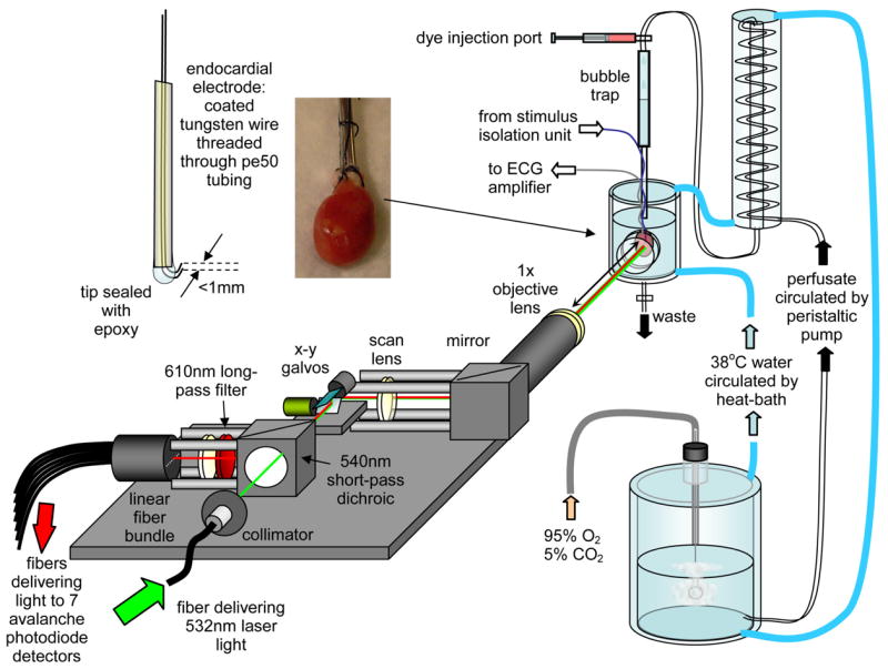
Laminar Optical Tomography system set up to image Langendorf perfused rat heart with endo-cardial electrode stimulation.

Once perfused and stabilized, the heart would begin to beat regularly and the EKG amplifier was adjusted to record a clear waveform. The heart was then regularly stimulated via computer control of a stimulus isolation unit (A360, WPI) delivering 0.11 ± 0.4 mA, 2ms pulses at between 4 and 6 beats per second to the endo-cardial electrode. Where necessary, a second bipolar electrode was immersed into the perfusion bath and carefully advanced until contacting the outer wall of the right ventricle. The stimulus isolation unit could then be switched between the endo-cardial or epi-cardial electrodes to allow imaging during stimulation of either wall of the heart. Proper synchronization of the heart to this pacing pattern was verified by examining the EKG. Diacetyl Monoxime (DAM) was then added to the circulating Tyrode’s solution in sufficient quantities to stop all mechanical movement of the heart (around 10mM). DAM acts as an electromechanical decoupler and so EKG activity and electrical wave propagation remain despite the lack of physical motion. 1ml of Di-4-ANEPPS VSD solution was then added to the in-coming perfusate (Invitrogen: D1199, 5μg in 1μl DMSO, diluted in 1ml Ringer’s solution). By illuminating with 532nm laser light and viewing through long-pass laser goggles it was possible to verify when the dye had uniformly perfused the right ventricle.

The heart was situated in a custom-modified double-walled glass perfusion bath (Radnoti Glass Technology Inc, CA). The water jacket was circulated with water at 38 degrees C to maintain stable temperature. A port in the side of the bath contained a glass tube capped with a thin glass cover-slip. This imaging port could be advanced through the double wall of the bath and positioned close to the surface of the heart, providing a clear view of the heart within the bath with minimal optical distortion.

2.2. Laminar Optical Tomography (LOT)

A schematic of the LOT system is shown in Fig. 2. LOT is similar to a confocal microscope, in that it uses galvanometer mirrors to scan a focused laser beam over the sample, and images the scanning spot back to stationary detectors. However, LOT does not scan the depth of the focus to achieve depth-resolution. Instead, it separately detects fluorescent light emerging from successive distances (up to 2.5mm) away from the scanning spot. This is achieved by having a linear fiber bundle in the plane usually occupied by a confocal pinhole. Each 200μm fiber in this bundle delivers light to an avalanche photodiode module (C5640-01, Hamamatsu) whose signal is then low-pass filtered and acquired in synchrony with the scanning galvanometer mirrors. Light that emerges from the tissue at further lateral distances from the scanning beam’s focus has, on average, scattered more deeply into the tissue than light emerging closer to the focus. By modeling this scattering using Monte Carlo methods, we can convert our raw data into a 3D image of the depth-resolved changes in the tissue [21–23, 27]. An example of simulated ‘spatial sensitivity functions’ for the detection of fluorescent light in heart tissue are shown in Fig. 3. Image reconstruction methods are described further below.

Fig. 3.

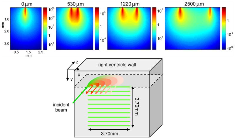
(top) Measurement sensitivity functions for different LOT source-detector separations, simulated using Monte Carlo modeling of fluorescent light propagation in rat heart at 532nm excitation and 610nm emission. (bottom) schematic of sequential line-scanning acquisition paradigm. After 800 sequential x-direction line-scans in 1.20 seconds, the LOT beam is shifted 370μm in the y direction and line-scan acquisition is repeated after triggering from the next heart beat stimulus.

To measure voltage-sensitive changes via Di-4-ANEPPS fluorescence, we used a 532nm Nd:YVO₄ laser, a 540nm short-pass dichroic filter and a 610nm long-pass emission filter. Note that these wavelength choices do not isolate the peak excitation (~480nm) and emission (~610nm) wavelengths of the dye, but instead target the falling sides of the excitation and emission spectra. This is because Di-4-ANEPPS fluorescence is modulated via a membrane potential dependent spectral shift, and not a change in amplitude. As such, a 540nm long pass filter alone would not provide a significant voltage-dependent signal [5]. Given our wavelength selection, an increase in membrane potential will result in a decrease in fluorescence signal.

The LOT source-detector separations used for these measurements were: 0, 0.23, 0.53, 0.86, 1.22, 2.04 and 2.49mm. These separations were chosen by selecting specific detection fibers from the linear fiber bundle in the image plane of the LOT system. The effective separations and field of view (3.7mm) were calculated from images of a ruler placed in the object plane. The LOT system acquired signals corresponding to all seven separations in parallel via a 64 channel 12 bit analog input data acquisition card (National Instruments PCI 6071E). The output from the EKG amplifier was connected as an 8^th input to the LOT system, allowing fully synchronized acquisition of a record of the heart’s response to pacing.

A rat heart typically beats 5–6 times per second, and the fine detail of the electrical propagation of each beat occurs on the scale of a few milliseconds. It was therefore necessary to implement a repetitive stimulus paradigm to capture details of the stimulated heart beat at very fast acquisition rates. The stimulus paradigm therefore proceeded as follows:

1. LOT was carefully aligned to image the surface of right ventricle overlying the endo-cardial electrode.

2. The LOT software was configured to wait for a trigger corresponding to the delivery of a stimulus pulse (from a second computer generating the cardiac stimulus).

3. When triggered, LOT rapidly acquired 800 lines scans in the horizontal plane of the heart at a rate of 667 lines per second (1.5ms per line-scan). While scanning, LOT acquired measurements 55 times within each 3.7mm line-scan. During these 800 line-scans, the heart beat between 5 and 7 times, depending on the stimulation rate.

4. LOT then moved the laser beam one step vertically down (370 μm), and then waited for the next heart beat stimulus to trigger the start of a further 800 line-scans.

5. This process continued until 10 vertical steps had been made, spanning a 3.7 × 3.7mm area overlying the endo-cardial electrode. This full acquisition sequence was repeated four times.

6. A second electrode was then introduced to the perfusion bath, and aligned to stimulate the epicardial surface of the right ventricle. The endo-cardial electrode was disconnected. The imaging process was then repeated with epi-cardial stimulation. If the heart was still functioning well, the electrodes were then swapped again and repeat measurements of endo-cardial stimulation were made.

The raw data were processed by analyzing the EKG signals measured through the 8^th acquisition channel of the LOT system. For heart beats where the EKG showed a normal response to pacing, the corresponding LOT data was extracted and temporally co-registered with all other normal EKG responses for a given line-scan y-location. Therefore, 5 to 7 heart beat responses could be extracted and averaged from one set of 800 line-scans, if the heart was responding well to pacing. The output in each of the 7 detector channels (corresponding to 7 different source-detector separations), for a given y-location line-scan set, was then a ~55 × 120 average response corresponding to 55 positions along the 3.7mm line-scanned and approximately 120 time-points (corresponding to ~180ms or the inter-beat interval). This analysis was repeated for the 10 vertical position line-scans, resulting in a final average data set consisting of 7 channels of 55 × 10 pixel square images over ~120 timepoints. The 55 x-pixels were then downsampled to 10 pixels to improve signal to noise, resulting in a data set of 7 × 10 × 10 × 120 measurements. These data provide the input to the 3D reconstruction algorithm described below. This data acquisition process is illustrated in Fig. 3.

2.3. Simulation of electrical propagation

In order to validate the depth-resolved imaging measurements made with LOT, we wished to compare our data to a physical model of electrical propagation in rat ventricle. We simulated propagation of electrical waves in a three-dimensional homogeneous 2mm thick slab of rat ventricular tissue using the generalized cable equation:

$$C_M{\partial }_t{V}_M(\overrightarrow{r},t)=-I_{\mathit{ion}}+\nabla \stackrel{\sim }{D}\nabla V_M(\overrightarrow{r},t)$$ (1)

where C_M denotes the membrane capacitance (set to 10⁻⁴ μF [25]), V_M the transmembrane potential, D the electrical diffusivity tensor and I_ion the total transmembrane ionic current, which determines the excitable properties of the tissue. The latter was calculated using a detailed electrophysiological model of rat ventricular myocytes [25]. This model includes a description of the different transmembrane channel currents, as well as of the ionic pumps and exchangers, and keeps track of the intracellular changes in ionic concentrations.

Propagation of electrical waves in cardiac tissue is much faster along than across muscle fibers, making the myocardium highly anisotropic. These fibers have a typical helical arrangement throughout the ventricles, with a counterclockwise rotation of the fiber direction from epicardium to endocardium by as much as 120° [16]. We accounted for this rotational anisotropy by an appropriate choice of the diffusivity tensor D as in [18]. In all simulations, the diffusivity in the longitudinal direction (along the muscle fibers) was 1 cm²/s and in the transverse direction (across the muscle fibers) was 0.11cm²/s. For these values, the conduction velocity of planar waves in longitudinal and transverse direction is 55 cm/s and 18 cm/s, respectively. Equation (1) was solved with an explicit finite-difference scheme (Euler method) in a slab of 1×1×0.2 cm³ and using a time step of 0.01 ms and a space step of 0.005 cm. The 3D simulations were coded in C and ran on a 52 parallel processor SunBlade grid.

As in the experiments, we investigated two types of electrical propagation: one resulting from epi-cardial stimulation (epicardium is defined as the z = 0 layer) and one resulting from endo-cardial stimulation. Both stimuli were applied in the middle of the concerned surface and had an amplitude of −50 pA and a duration of 2 ms.

In addition to allowing us to evaluate how well our experimental data agrees with classical electrical modeling of cardiac activity, we can also use these simulations to evaluate our optical imaging performance: This physical model of the anticipated behavior of electrical propagation in rat ventricle can be used as a set of surrogate 3D data to evaluate the likely best-case performance of LOT for cardiac imaging.

2.4. LOT image reconstruction and electro-optical modeling

Fluorescence diffuse optical imaging to date has generally attempted to reconstruct the absolute structure of a fluorescent target within a fairly large, scattering tissue volume [28]. For LOT of fluorescent voltage sensitive dyes in cardiac tissue, the image reconstruction is slightly different: Firstly, we are seeking to reconstruct the perturbation in the fluorescent intensity of the tissue, and not the absolute fluorescent structure. Secondly, although fluorescence emission from a fluorophore is isotropic, a diffusion approximation-based model of light propagation cannot be used for LOT. This is because the trajectories of the highly directional light entering the cardiac tissue (and therefore also the directionality of the detected photons) cannot be modeled using the diffusion equation over distances of a few millimeters (of the order of the scattering length of tissue). The numerical aperture of the LOT system used for these experiments is 0.05 (so light is almost collimated), and detector separations were all less than 2.5mm. For absorption imaging using LOT, the model of light propagation carefully accounts for the directionality of each photon, and therefore its likelihood of changing its direction to reach the detector [21, 27]. For fluorescence LOT, this directionality is not as important, but the initial distribution of incident photons can only be modeled by radiative transport, and so we use Monte Carlo modeling for this purpose.

We formulate our image reconstruction approach by starting from the following description of steady-state fluorescence detected from a scattering medium:

$$F_{x,m}(r_d-r_s,t)=\int p_{x,m}(r,t)H_x(r-r_s)E_m(r_d-r)d^{3}r$$ (2)

where

$$p_{x,m}(r,t)={\epsilon }_x(r,t)c(r){\eta }_m(r,t)$$ (3)

where H is the distribution over r of excitation light in the medium resulting from a source at position r_s (and is a function of the tissue absorption and scattering coefficients μ_a and μ_s, the anisotropy g and refractive index n of the tissue at the excitation wavelength). E is the distribution of emission light in the medium from fluorescence sources within the medium, detected at position r_d (and is a function of the μ_a, μ_s, g and n of the tissue at the emission wavelength) [29]. ε_x is the extinction coefficient of the dye (a function of the excitation wavelength), c is the concentration of the dye, and η_m is the quantum efficiency of the dye’s fluorescence (a function of the emission wavelength). The time-dependence of p_x,m(r,t) denotes changes that occur due to changes in membrane potential.

We make the following assumptions: That the concentration of the dye does not vary over time, but only that the excitation and emission spectra of the dye vary with changes in membrane potential V(r,t). Further, we assume that relative changes in quantum efficiency are greater than changes in the extinction coefficient (consistent with transmission measurements [5]), such that p_x,m(r,t) ≈ ε_x(r)c(r)η(r,t), and further that p_x,m(r,t) ∝ V(r,t), or p_x,m(r,t) = wV(r,t) where w is a scaling constant [30, 31]. We also assume that the spectral shift in emission light (the underlying mechanism causing the change in η_m) is not sufficient to change the average tissue optical properties experienced by the detected emission light. Under these assumptions, H_x and E_m will be temporally invariant, because scattering and absorption within the tissue is not varying sufficiently during the heart beat to alter the distribution of excitation or emission light within the tissue (note that the heart does not actively contract in the presence of DAM). Therefore, if we are looking at changes in the intensity of fluorescent light, we get:

$$\mathrm{\Delta }{F}_{x,m}(r_d-r_s,t-t_0)=w\int \mathrm{\Delta }V(r,t-t_0)H_x(r-r_s)E_m(r_d-r)d^{3}r$$ (4)

H and E can be modeled using Monte Carlo methods. However, their calculation requires accurate estimates of the optical properties of heart tissue at the excitation and emission wavelengths. These estimates were obtained using a multi-distance frequency domain spectrometer system in the following way: 6 hearts which had undergone perfusion, dye injection and measurements with LOT were collected and rapidly frozen after each experiment. All 6 hearts were then thawed and wrapped together in saran wrap to make a ~ 4cm by 3cm block of approximately homogenous tissue. This block was measured and values of μ_a and μ′ _s = μ_s(1−g) were calculated for wavelengths between 670nm and 830nm. These values were then fit to the spectrum of myoglobin and a scatter model to yield estimates at 532nm: μ_a = 0.880mm^−1, μ′_s = 0.742mm⁻¹, g = 0.9 and > 610nm: μ_a = 0.165mm^−1, μ′ _s = 0.630 mm⁻¹, g = 0.9.

Based on these optical properties, we used Monte Carlo modeling to calculate the forward fluence in the tissue corresponding to illumination with 0.05 NA focused light. H_x(r−r_s) is given by the distribution of 532nm excitation light, incident at position r_s. Exploiting reciprocity, E_m(r_d−r) is equivalent to the forward fluence of >610nm light incident on the tissue at position r_d (since the probability that a photon from position r will be detected at position r_d (within NA 0.05) is approximately the same as the probability of a photon entering at r_d and reaching position r). Multiplied together at every r voxel, H_x(r−r_s) and E_m(r_d−r) combine to become measurement sensitivity functions J_x,m(r_s,r_d,r), corresponding to the spatial sensitivity of the fluorescence intensity measurement between a source at r_s and a detector at r_d owing to a change in p_x,m at position r. Fig. 3 shows plots of J_x,m(r_s,r_d,r). So where:

$$J_{x,m}(r_s,r_d,r)\approx H_x(r-r_s)E_m(r_d-r)$$ (5)

Eq. (4) becomes:

$$\frac{1}{w}\mathrm{\Delta }{F}_{x,m}(r_d-r_s,t-t_0)=\int J_{x,m}(r_s,r_d,r)\mathrm{\Delta }V(r,t-t_0)d^{3}r$$ (6)

This linearized equation can be inverted to yield images of the change in V from measurements of change in fluorescence emission at positions r_d in response to illumination at positions r_s. For absorption imaging, we found that it was advantageous to introduce a normalization factor into this equation, such that the percentage change in measurement is the input [21], rather than just the difference. This has significant benefits including that differences in detector-specific gains can be compensated for, as well as that smaller absolute values in signal corresponding to more distant detectors (and therefore deeper tissue) can more strongly influence the image reconstruction. So for fluorescence imaging, where we are investigating perturbations in fluorescence, the image reconstruction therefore becomes:

$$\frac{\mathrm{\Delta }{F}_{x,m}(r_d-r_s,t-t_0)}{F_{x,m}(r_d-r_s,t_0)}=\frac{\int J_{x,m}(r_s,r_d,r)\mathrm{\Delta }V(r,t-t_0)d^{3}r}{L_{x,m}(r_s-r_d)}$$ (7)

where L_x,m(r_s−r_d) is calculated from the Monte Carlo simulation to represent the steady-state fluorescent field. Note that the values of F_x,m used to normalize Eq. (7) incorporate background subtraction for each channel, since baseline signals on each detector channel are non-zero owing to residual room light, and are a function of the level of gain on each channel. D(r_s,r_d) is measured by acquiring a standard data set while the laser source is blocked, and F_x,m (r_s−r_d, t₀) = F′_x,m (r_s−r_d, t₀) − D(r_s,r_d) where F′_x,m represents the raw measured signal. Note that the scaling constant w cancels in this normalized case.

We chose to invert Eq. (7) using Tikhonov regularization, solving for Δ V(r,t−t₀). In matrix form the problem becomes:

$$\frac{\mathrm{\Delta }\mathbf{V}}{\mathbf{S}}={\mathbf{J}}^{\text{T}}{(\mathbf{J}{\mathbf{J}}^{\text{T}}+\alpha I)}^{-1}\frac{\mathrm{\Delta }\mathbf{F}\cdot \mathbf{L}}{({\mathbf{F}}_0)\cdot \mathbf{S}}$$ (8)

S = S(r) is an additional scaling factor which can be varied to add spatial weights to the reconstruction. This scaling factor was incorporated into the image reconstruction to provide so-called ‘depth-dependent regularization’ as a means to further increase the influence of deeper regions on the image reconstruction solution [32, 33]. Our choice to incorporate S was the result of imaging performance tests performed on our simulated electrical data as described further below.

Once calculated using Eq. (5), J_x,m(r_s, r_d, r) can be used to simulate forward ‘optical’ data from the electrical propagation modeling results from Eq. (1). Where Δ V_M(r,t−t₀) represents simulated changes in membrane potential within the heart wall, simulated boundary data $\mathrm{\Delta }{F}_{x,m}^{\mathit{sim}}$ equivalent to our LOT data can be generated using:

$$\frac{\mathrm{\Delta }{F}_{x,m}^{\mathit{sim}}(r_d-r_s,t-t_0)}{F_{x,m}^{\mathit{sim}}(r_d-r_s,t_0)}=\frac{\int J_{x,m}(r_s,r_d,r)\mathrm{\Delta }{V}_M(r,t-t_0)d^{3}r}{L_{x,m}(r_s-r_d)}$$ (9)

This approach allows us to compare measured LOT data with the simulated electrical model of propagation in both data-space and image-space. In data space (s,d), comparing ΔF^sim_x,m/F ^sim_x,m to Δ F_x,m/F_x,m, we can examine how accurately our measured experimental data agree with the simulation of electrical activity, irrespective of our chosen 3D reconstruction method (assuming that our optical model is adequate). By reconstructing the simulated data ΔF^sim_x,m/F^sim _x,m using Eq. (8), we can then compare ΔV^sim in ‘reconstructed image space’ to ΔV_M(r). This ‘image space’ (r) comparison, allows us to evaluate the ‘best possible performance’ of our current LOT system configuration and image reconstruction algorithm.

All reconstructions were performed side by side on both simulated forward data based on our electrical model, and our experimental data to allow evaluation of any distortions or variations in sensitivity and resolution that were arising only because of our measurement-geometry and image reconstruction parameters. In performing these tests, we found that the depth-dependent regularization factor S was needed to more accurately reproduce the spatiotemporal behavior of our electrical model, which was otherwise distorted because deeper signals were resolved with lower amplitudes than the original pattern of propagation. Once we had derived image reconstruction parameters that satisfactorily reproduced the electrical propagation patterns from our electrical model, exactly the same image reconstruction parameters were used to reconstruct our LOT measured data. For the results shown, we used S = e 0.78z where z is depth in millimeters. These results will be shown and discussed in more detail below.

In practice, J_x,m was calculated on a 50μm 3D grid and then down-sampled to match the resolution of the source-positions on the surface of the heart in the x-y plane, and to 200μm slices in depth (e.g. each reconstruction voxel was 370 × 370 × 200μm). The data were reconstructed into a volume consisting of a 2mm thick slab whose x-y area spanned the area sampled by all source and detector positions, such that the size of the J matrix in Eq. (8) was 7 × 14 × 10 × 10 corresponding to 7 source-detector separations and x, y and z. The size of the measured data matrix ΔF/F was 7 × 10 × 10 × 120 corresponding to 7 source-detector separations, x-source positions, y-source positions and time-steps. When solved, the size of the resulting image ΔV was 14 × 10 × 10 × 120 corresponding to x, y, z and time-steps. All data acquisition, analysis and image reconstruction was performed using Matlab^™. Tikhonov inversion took 3 seconds on a 2GHz AMD Turion 64 laptop with 2Gb RAM.

3. Results

3.1. Electrical simulation

Fig. 4 shows movies of the simulation of electrical excitation propagation in a model of the right ventricle wall of rat heart in response to epi- and endo-cardial point stimulation. The volume-averaged time-course of the electrical response within the first 500μm on the epi-cardial and endo-cardial faces are also shown. These propagations assume an ideal case of tissue with flat sides and linear transmural fiber rotation [12]

Fig. 4.

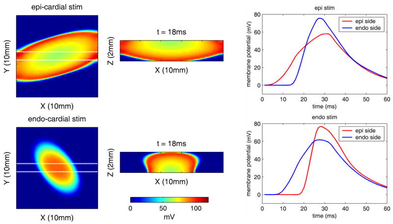
[Movie 1.1Mb.avi] Electrical simulation of wave propagation resulting from epi-cardial (top row) and endo-cardial (bottom row) stimulation, for properties consistent with the right ventricle of a rat heart. Left column: X-Y view of changes in the top 500μm of the epi-cardial surface at 18ms after stimulation, middle: cross-sectional X-Z view at the same time-point between the Y-locations indicated by the white dotted lines in the x-y plane images (epi-cardial surface is at the top). Right: timecourses of changes in the upper 500μm of the epi-cardial surface and lower 500μm of the endo-cardial surface for epi (top) and endo (bottom) cardial stimulation, averaged over the 10 × 10mm X-Y area.

The electrical waves have an ellipsoidal shape due to the tissue’s anisotropy: The transmural rotation of the fiber’s orientation results in different preferential directions of propagation on the epi- and endocardium, leading to different orientations of the waves as observed in the left panels. When pacing the epicardium, the wave gradually spreads both in the lateral (x-y) and depth (z) directions, resulting in the slow rise observed in the time course on the epi-side (red trace in top right panel). By the time the wave reaches the endocardium it has substantially propagated in the xy-direction (middle panel top row), resulting in a faster increase in the time course on the endo-side (blue trace in top right panel). The opposite is true for a wave initiated on the endocardium (lower panels).

In the experimental case, the endo-cardial surface is rough and fibrous, and the location and extent of the stimulation delivery is less well defined. In practice, the right ventricle is also stretched slightly over the electrode and therefore likely to be distorted relative to this simulation. Nevertheless, this simulation can provide us with a ‘best-case’ representation of anticipated endo- and epi-cardial stimulation, and provides a realistic model of the likely propagation speed and extents of electrical propagation.

3.2. LOT raw data

We can use the electrical model data shown in Fig. 4 to simulate the likely optical data that [using Eq. (9)]. We can compare the information we would measure with LOT ΔF^sim_x,m/F^sim _x,m content of this data with the raw data measurements ΔF_x,m/F_x,m from LOT. Fig. 5 compares raw LOT experimental data, for five source-detector separations, to simulated raw data based on our electrical model. These data sets were selected from two different hearts, and each set is the average of 72 repeated stimuli. These sets were chosen as they show the clearest and most uniform transmural response to epi- or endo-cardial stimulation, analogous to our electrical simulation. In other data sets, our ability to visualize clear transmural propagation depended on the relative positions of the stimulation electrode and measurement area, such that in other cases transverse and even 3D re-entering waves were seen.

Fig. 5.

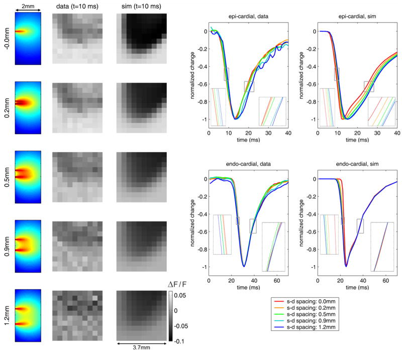
[Movie 1.6Mb.avi] Comparison of raw LOT data to optical forward-model data based on electrical model. Left: 10 × 10 pixel raw LOT images for 5 different source-detector separations for measured and simulated epi-cardial stimulation (fractional change). Corresponding depth-resolved sensitivity functions are also shown (far left). Right: time-courses extracted from raw and simulated data for five source-detector separations. Insets show closeups of regions highlighted by small grey squares.

The animation on the left of Fig. 5 shows the propagation of the measured ΔF_x,m/F_x,m and simulated ΔF^sim_x,m/F^sim _x,m response to epi-cardial stimulation for one experiment. Decrease in signal denotes an increase in membrane potential. The site of epi-cardial excitation is just out of the field of view at the top. The electrical simulation excitation position was adjusted to an equivalent field of view. The depth-sensitivity functions J_x,m for each measurement are also shown.

If we extract the mean time-course of the measurements for each source-detector separation we can clearly see that the raw data includes information regarding the direction of propagation of the transmural electrical wave [15]. These data are shown normalized to their minimum value for all channels. For epi-cardial stimulation, for both the measured and simulated data, during the initial reduction in signal the first channel to change is that corresponding to the zero source-detector separation, which samples the more superficial tissue. The signals from the wider source-detector separations are successively delayed (see inset). Similarly on the return to baseline, the zero separation signal begins to rise first, followed by the wider separations, in agreement with the electrical model data. Similarly, for the endo-cardial stimulation, the signal can be seen to change first in for the widest source-detector separation in both the measured and simulated data. During the return to baseline, all of the traces overlap temporally. This result confirms that the values that we measured in the right ventricle of the rat heart are consistent with our electrical and optical models, and also confirms that the direction of propagation of the transmural electrical wave can be deduced from raw LOT data.

The transmural dynamics of electrical waves in perfused heart have not previously been well characterized. The marked differences in the dynamics of the return-to-baseline of the electrical response for epi-cardial versus endo-cardial stimulus are therefore quite surprising. We believe that this behavior can be explained in the following way: The epi-cardial model (1.1Mb movie) in Fig. 4 shows that the wave spreads out laterally faster than advancing forward in the z direction. The back of the wave (the propagation of the relaxation) therefore propagates almost uniformly in the z direction. This leads to clearly differentiated depth-specific differences in timing as the response to epi-cardial stimulation recovers. The endo-cardial stimulation, conversely propagates predominantly in the -z direction at first, spreading out laterally only later. This means that the positive wavefront is still traveling laterally, and even curling back to the endo-cardial surface, while the propagation of relaxation advances towards the epi-cardial surface. Because our time-courses show the average data from all source positions over the area measured, we believe that these two effects combine causing it to appear that the relaxation of the endo-cardial response occurs fairly instantaneously at all depths

3.3. 3D LOT image reconstructions

The raw data shown in Fig. 5 can be reconstructed using Eq. (8) to yield 3D images of transmural electrical propagation. Fig. 6 compares the 3D behavior of the electrical waves resulting from epi-cardial and endo-cardial stimulation for experimental data. We chose to based on our electrical simulation in also reconstruct the modeled forward-data ΔF^sim_x,m/F^sim_x,m order to understand the ‘best case’ performance of LOT. As with any reflectance-geometry optical tomography method, the accuracy and resolution of LOT degrades with depth. By reconstructing simulated data derived from our electrical forward model using exactly the same reconstruction parameters, we can understand any likely distortion resulting from the reconstruction process. We display the data as 40% isosurfaces (where red denotes a higher membrane potential) and as averages over x and y which show the depth-propagation of the wave as a function of time (referred to here as Z-T plots). Reconstructed images were interpolated onto a finer spatiotemporal grid prior to display.

Fig. 6.

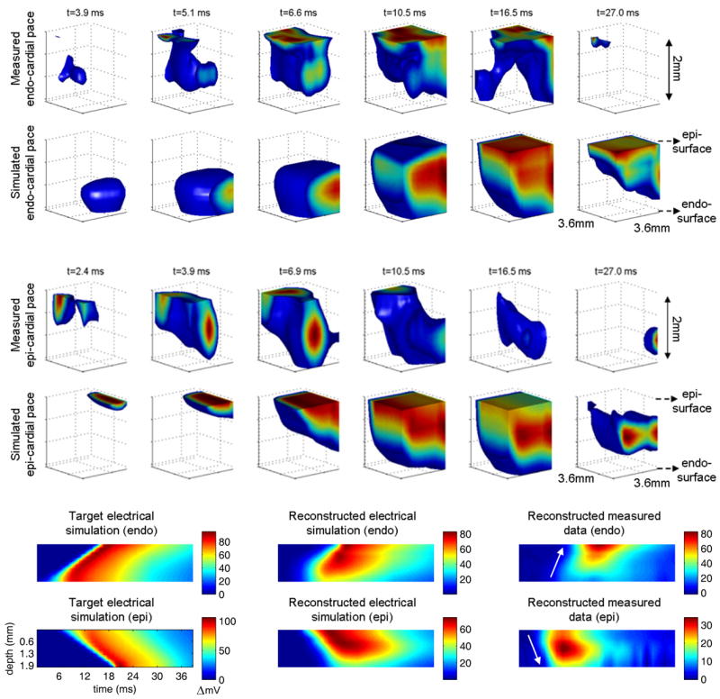
[Movie 1.6Mb avi] 3D reconstructions of transmural electrical propagation in the right ventricle of a rat heart. Top row shows reconstructions of data acquired during endocardial stimulation, along with corresponding reconstructions of simulated optical data based on our model of electrical propagation. Middle row: equivalent results for epi-cardial stimulation. Bottom row: Z-T plots showing the average signal (over x and y) as a function of depth and time. The direction of the red stripe demonstrates the direction of propagation. Left: shows the ‘target’ behavior that we expect from our electrical model, center: shows the result of reconstructing simulated optical data based on the electrical model (to explore the ‘best case’ imaging performance), and right: shows experimental results for epi- and endo-cardial stimulation.

Our results verify that the endo-cardial stimulation results in a wave which propagates from deeper to shallower layers of the heart wall. There are some irregularities to the wavefront, which we expect from comparisons of measured data to simulated data. These are most likely due to tissue heterogeneities which are not accounted for in the mathematical model. For the reconstruction of the ‘ideal case’ electrical simulation we see some distortion to the previously smooth wavefront. Looking at the Z-T plots we can see that the signal in the deepest layers (from 1.8 – 2mm) is underestimated for the electrical simulation, and therefore this is also likely to be the case in our experimental data. The same is true of the epi-cardial stimulation images; the direction of propagation is clear, but there is some wavefront distortion in the experimental data images as with the endo-cardial data. The poorer sensitivity to the deepest layers is also clear from the reconstruction of the electrical model data. Nevertheless, the direction of propagation, as well as a measure of the propagation speed can be determined from these images: By evaluating the gradient of the wavefront signal in these Z-T plots, we estimate that the velocities of transmural propagation for epi- and endo-cardial stimulation to be +45 and −51cm/s respectively which, while higher than in our electrical simulation, are within a physiologically reasonable range [31].

4. Conclusion

We have demonstrated that it is possible to determine the direction of propagation of an electrical wave within the cardiac wall using non-contact optical measurements of the epi-cardial surface. By using a scanning laser-based imaging technique we were able to achieve both the high frame rates and the depth-sensitivity required to probe beneath the epi-cardial surface and resolve the shapes of transmural electrical waves following a point stimulus. The good agreement between our experimental data and our electrical model of propagation serves as important validation of the electrical model and the chosen model parameters, as well as the integrity of our forward optical model and experimental setup. By reconstructing forward data based on our electrical model we were able to evaluate the likely accuracy of our 3D imaging performance.

Future work will incorporate the use of newer NIR and red-shifted VSDs to allow significantly improved penetration of light into the cardiac wall. Our new second-generation LOT system will allow increased fields of view and source-detector separations. Using red-shifted dyes we expect to be able to image thicker samples (and therefore larger hearts). We also hope that these new tools will allow single-trial imaging, whereby it is not necessary to repeat and average the same stimulation paradigm multiple times, allowing more complex cardiac behavior to be examined in detail. The results shown in this study represent the first step towards a versatile imaging approach to non-contact and non-destructive imaging of 3D electrical activity dynamics in the heart.