Folding thermodynamics of pseudoknotted chain conformations

Abstract

We develop a statistical mechanical framework for the folding thermodynamics of pseudoknotted structures. As applications of the theory, we investigate the folding stability and the free energy landscapes for both the thermal and the mechanical unfolding of pseudoknotted chains. For the mechanical unfolding process, we predict the force-extension curves, from which we can obtain the information about structural transitions in the unfolding process. In general, a pseudoknotted structure unfolds through multiple structural transitions. The interplay between the helix stems and the loops plays an important role in the folding stability of pseudoknots. For instance, variations in loop sizes can lead to the destabilization of some intermediate states and change the (equilibrium) folding pathways (e.g., two helix stems unfold either cooperatively or sequentially). In both thermal and mechanical unfolding, depending on the nucleotide sequence, misfolded intermediate states can emerge in the folding process. In addition, thermal and mechanical unfoldings often have different (equilibrium) pathways. For example, for certain sequences, the misfolded intermediates, which generally have longer tails, can fold, unfold, and refold again in the pulling process, which means that these intermediates can switch between two different average end-end extensions.

I. INTRODUCTION

RNA pseudoknots are simple tertiary structures formed by the base pairing of nucleotides of a loop (hairpin, internal, bulge, or bifurcated) with nucleotides outside that loop. The simplest and most general is the hairpin (H)-type pseudoknot which includes only two loops and two stems: nucleotides of the hairpin loop base pair with nucleotides of the end of the chain. RNA pseudoknots are found to play a variety of important roles in cellular function: they are involved in translational regulation, viral replication, and some catalytic functions of ribozymes. In the present study, we develop a statistical mechanical thermodynamic model for RNA pseudoknots. Such a model may lead to a better understanding of RNA pseudoknot function.

Unlike secondary structures, which can be divided into nearly independent elements: loops, stems, and dangling segments, pseudoknot structures involve interactions which tie together secondary structure subunits (e.g., stems, loops) and make them strongly correlated. A result of the correlation between different structural subunits is the nonadditivity of chain entropy and free energy, i.e., the entropy and free energy of a pseudoknot cannot be calculated as a sum of entropies and free energies of each individual secondary structural subunits. For an H pseudoknot, which consists of two helix stems and two loops, the enthalpy can be estimated from the known energy parameters for helix stems,^1–3 but the calculation of the pseudoknot entropy requires a model that can account for the nonadditivity of chain entropy.

The estimation for the loop entropy for H-type pseudoknot was first attempted by Gultyaev et al. (1999).⁴ The authors used the Jacobson-Stockmayer approximation⁵ for the loop entropy and fitted parameters from the stability data of known pseudoknots. Though the proposed thermodynamic parameters were shown to give much better approximation than the previous one,⁶ the excluded volume effect (impossibility for two monomers to occupy the same site) has not been taken into account explicitly. Recently, a three-dimensional (3D) lattice-based statistical mechanical model⁷ was developed to explicitly take into account the excluded volume effect for pseudoknots. However, the model disallows the formation of possible partially unfolded and misfolded intermediate states in the pseudoknot folding process.

In this paper, we develop a statistical mechanical model that can treat (a) the excluded volume effect, (b) the nonadditivity arising from the correlation between different structural subunits, and (c) the formation of partially folded and misfolded intermediates. Though our major focus here is on the H pseudoknot and the misfolded and the partially folded states, the methodology developed in this work is general and can be extended to treat more complex pseudoknotted structures. In addition, the method uses graphical representation for intrachain contacts and is thus independent of any specific chain representation. For illustrations, we use two-dimensional (2D) lattice chain conformations, where the excluded volume effect is accounted for by configuring the chain conformations as self-avoiding walks in a 2D lattice.

The paper is organized as follows. We first develop a statistical mechanical model for the conformational entropy of pseudoknotted structures. We then apply the model to study both the thermal and the mechanical folding free energy landscapes and folding thermodynamics for pseudoknotted structures. An advantage of the present theory is its ability to treat the complete conformational ensemble for the pseudoknotted structures (and the secondary structures), including all the partially folded and misfolded states.

II. GRAPH-THEORETIC APPROACH TO POLYMER THERMODYNAMICS

At the center of the statistical thermodynamics is the partition function Q(T), defined as the weighted sum over all the possible conformational states,

$$Q(T)=\sum _{\text{conf}}{e}^{-E/k_{B}T},$$ (1)

where k_B is Boltzmann’s constant, T is the temperature, and E is the energy of an individual conformation. We use the graph-theoretic approach^8–12 to calculate the partition function. A polymer graph gives the intrachain contacts and is thus a convenient way to represent RNA structures. It consists of vertices which represent monomers, connected by straight line links as the (covalent) bonds between monomers. Monomers in spatial contact (base pairs in nucleic acids such as RNAs) are connected by curved links. There are three possible relationships between two contacts: nested, unrelated, and crossing linked.⁹ Secondary structures involve only nested and unrelated contacts, while tertiary folds such as pseudoknots involve crossing links.

In terms of the polymer graph, the partition function can be calculated as a sum over all the possible graphs, which is computationally more efficient than over all the possible conformations,

$$Q(T)=\sum _{\text{graph}}\mathrm{\Omega }{e}^{-E/k_{B}T},$$ (2)

where Ω is the number of chain conformations that satisfy the intrachain contacts defined in the graph. Since the energy E is determined by the intrachain contacts, a graph represents an equal-energy conformational ensemble. The key issue for the method is how to calculate the conformational count Ω for the given graph. We start from the simple H pseudoknot and then generalize the method to treat more complex pseudoknots.

III. CONFORMATIONAL ENTROPY OF PSEUDOKNOTS

The H pseudoknot consists of two stems and two loops, as shown in Fig. 1. For mathematical convenience, we cut off dangling tails, leaving only one bond of each tail to account for the excluded volume interactions between the tails and the rest of the structure. We call such tail-free structure “structure element.” A full structure consists of two parts: structure element and the tails (in the 5′ and 3′ terminal regions of the nucleotide chain). Loops A and B share the common single-stranded (interfacial) chain segment and are also constrained by the helical stems, therefore, the conformations of loops A and B are strongly correlated with each other. The basic idea in our pseudoknot conformational entropy theory is to divide a pseudoknot into three components, namely, the enlarged interface (shown as solid lines in Fig. 1), and the two noninterfacial free loop segments F_A and F_B (shown as dashed lines in Fig. 1) of lengths f_A and f_B, respectively. The enlarged interface includes two stems of lengths n₁ and n₂, the single-stranded interfacial segment of length l, and the tail monomers 0 and N in Fig. 1.

FIG. 1.

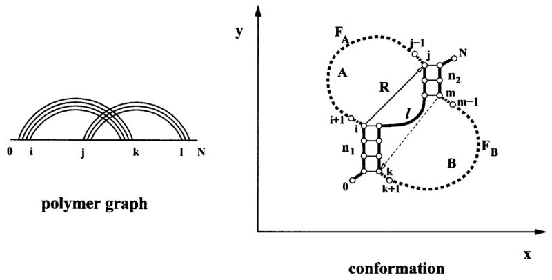
The polymer graph and the structure of an H pseudoknot. The pseudoknot is divided in our theory into enlarged interface (bold lines) and two free loop segments F_A and F_B (dashed lines). The coordinate system is chosen so that the y axis is along the first pseudoknot stem. The number of free loop segment conformations is a function of the length of the free loop segment and the end-end vector R.

A great challenge in the entropy calculation is how to treat the excluded volume effect. According to the decomposition of the pseudoknot structure, we classify the excluded volume interactions into two types: (a) between the interfacial monomers (i.e., monomers in the enlarged interface) and (b) between the free loop monomers (i.e., monomers in the free loop segments) and between the free loop monomers and the interfacial monomers. We treat the former (type a) excluded volume effect by considering all the viable self-avoiding enlarged interface conformations (denoted as I) that (i) do not make self-contacts other than those specified by the graph and (ii) allow viable positioning of monomers i + 1, j−1, k+ 1, and m−1 without causing additional contacts. In terms of I, we compute the number of conformations Ω_P of the pseudoknot as a sum over all the possible viable conformations I of the enlarged interface,

$${\mathrm{\Omega }}_P=\sum _{\mathbf{I}}{\mathrm{\Omega }}_f(\mathbf{I},f_A)·{\mathrm{\Omega }}_f(\mathbf{I},f_B),$$ (3)

where Ω_f(I, f_A) and Ω_f(I, f_B) are the numbers of conformations of the free loop segments F_A and F_B for a given I, respectively. The later (type b) excluded volume effect plays a crucial role and should be taken into account in the computation of Ω_f(I, f_A) and Ω_f(I, f_B).

In Eq. (3), we neglect the volume exclusion between the free loop segments F_A and F_B. This is because, first, the free loop segments are spatially separated by the enlarged interface and, second, the steric hindrance between each free loop segment and the interface is accounted for in the calculation of Ω_f (see next section). For very large loops and long free loop segments, the volume exclusion between F_A and F_B may become important. However, in that case, the chain entropy is large, so the error caused by neglecting the F_A − F_B volume exclusion is relatively small as compared with the (large) chain entropy.

If one has a table for Ω_f(I, f_A) and Ω_f(I, f_B) for all the possible free loop segment lengths f_A and f_B and enlarged interface conformations I, the computation of Ω_P for the given graph (pseudoknot) from Eq. (3) would be efficient and straightforward. However, the number of possible parameter sets (f_A, f_B, I), grows exponentially with the length of the interface, which makes the tabulation of Ω_f for all the possible parameter sets practically impossible. In the next section, we develop a method to approximate the conformational count Ω_f for the free loop segments. The derived expression for Ω_f would be mathematically convenient and computationally efficient.

A. Number of conformations of a free loop segment

Because of the obviously equal roles of loops A and B in Fig. 1, instead of calculating Ω_f for the two loops separately, we focus on the calculation for one of the loops, namely, loop A. In what follows, we derive an approximate expression for the number of conformation Ω_f for the free loop segment F_A in loop A. The derived result for loop A would be equally applicable to loop B.

Strictly speaking, the number of conformations Ω_f = Ω_f(I, f_A) for the free loop segment F_A (in Fig. 1) is a function of the enlarged interface conformation I, which is dependent on the interface length l and the length of the two helical stems (n₁ and n₂), etc. However, as an approximation, we replace the I dependence by the end-end vector R dependence; see the vector from i to j in Fig. 1. The end-end vector for F_B is shown as the dashed line in Fig. 1. We further define a two-dimensional Cartesian coordinate system by choosing the y axis along stem 1 (directed upward), as shown in Fig. 1; vector R can be described through the components: R= (x, y), where x= x_j − x_i and y = y_j − y_i in Fig. 1. In terms of the components of R, we reduce the Ω_f function from a large parameter space (for the interfacial chain conformations I) to a much smaller two-variable parameter space [for R= (x, y)],

$${\mathrm{\Omega }}_f(\mathbf{I},f)\simeq {\mathrm{\Omega }}_f(\mathbf{R},f)\to {\mathrm{\Omega }}_f(x,y,f).$$

Since the information about I is now embedded in R, for an f_A-mer free loop segment F_A with fixed end-end vector R= (x, y), we compute the conformational count Ω_f(R, f_A) as an average over all the possible enlarged interface conformations I with the fixed end-end vector R,

$${\mathrm{\Omega }}_f(\mathbf{R},f_A)\simeq \frac{{\sum }_{\mathbf{I}}{\mathrm{\Omega }}_f(\mathbf{I},f_A)}{{\mathrm{\Omega }}_{\mathbf{I}}},$$

where Ω_I is the number of all the viable enlarged interface conformations with the given R= (x, y), and Σ_I is the sum over all these conformations. Physically, the calculated Ω_f(x, y, f_A) function is the average conformational count of F_A for each given enlarged interface conformation I.

In fact, the first helix stem length n₁ affects the conformational count of F_A only through weak excluded volume interactions mainly located around the junction between the helix and F_A. For the helix stem length n₁ ⩾ 2 base stacks, the conformational count for F_A is nearly independent of n₁. In our calculation, we choose n₁ = 3 base stacks and fix the orientation of helix stem 1 to be upright (in the y direction). We then enumerate all the possible conformations of the enlarged interface for all the possible values of l and n₂ such that 1 ≤ l+ n₂ ≤ 10. For each enlarged interface conformation I and the given free loop segment length f_A(f_A ≤ 21), we calculated the number of free loop segment conformations Ω_f(I, f_A) by means of exact computer enumerations of self-avoiding walks on 2D lattice.

As an illustration, in Fig. 2(a), we show all the viable conformations of the enlarged interface with fixed n₁ = 3 (base stacks) and end-end vector R= (x, y) = (3, 4). For the given end-end vector R, the length n₂ of stem 2 has only four possible viable values: n₂ = 1, 2, 3, 4, and the length of the single-stranded interfacial segment is restricted by l≤ 10 − n₂. The possible interface conformations are represented as self-avoiding random walks on the dashed grid (with one of the conformations drawn as solid line). Figure 2(b) shows how the volume exclusion between the free loop segment and the interface determines the viability of conformations. The depicted conformation of the enlarged interface in Fig. 2(b) is not viable because it is impossible to position monomer s in the square lattice without making additional contacts with the single-stranded interfacial segment.

FIG. 2.

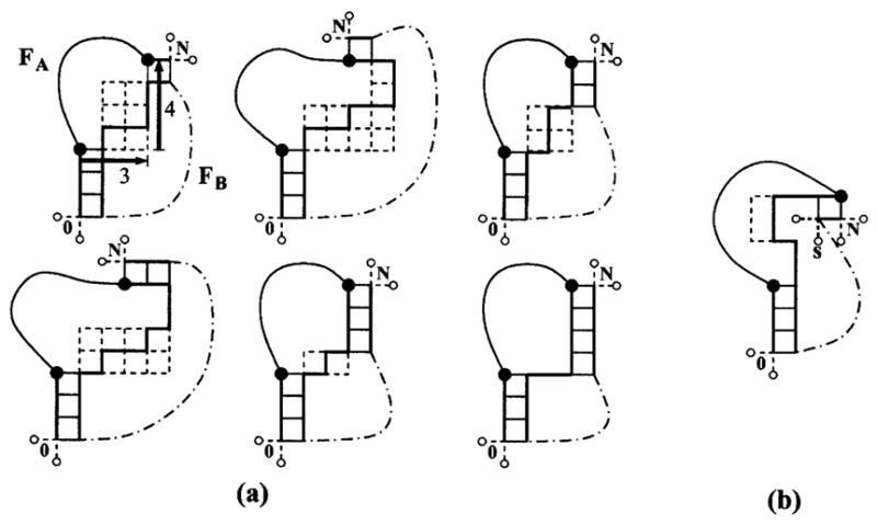
(a) All the viable conformations of possible enlarged interfaces that give end-end vector R= (x, y) = (3, 4) for the free loop segment F_A. The position and length of the first stem are fixed. Big black circles denote the end monomers of the free loop segment F_A. Part of the 2D lattice which can be covered by the viable conformations of the interfacial segment for possible length and position of the second stem is shown with dashed lines. The dash-dotted line denotes the F_B segment. Two possible positions for 0 and N are shown for each interfacial conformation. (b) An example of the conformation of the enlarged interface which is not viable because all the possible positions of the monomer s would make an additional contact with the interfacial segment.

B. Number of conformations of pseudoknots

1. Pseudoknot with two stems

With the reduced function Ω_f(R, f) for free loop segments F_A and F_B, we obtain the conformational count of the pseudoknot from Eq. (3) by replacing Ω_f(I, f) by Ω_f(R, f),

$${\mathrm{\Omega }}_P\simeq \sum _{\mathbf{I}}{\mathrm{\Omega }}_f({\mathbf{R}}_A,f_A)·{\mathrm{\Omega }}_f({\mathbf{R}}_B,f_B),$$

where R_A and R_B are the end-end vectors of the free loop segments F_A and F_B, respectively, for a given conformation I of the enlarged interface. As shown in Fig. 1, R_A is the vector i→j and R_B is the vector m →k.

The method can be generalized to treat more complicated pseudoknots. Here we demonstrate how to extend the method to treat pseudoknots with an internal loop in the stems [Fig. 3(a)]. Such “pseudoknot” conformations are important because they may emerge as partially folded or misfolded intermediates in the pseudoknot folding process.

FIG. 3.

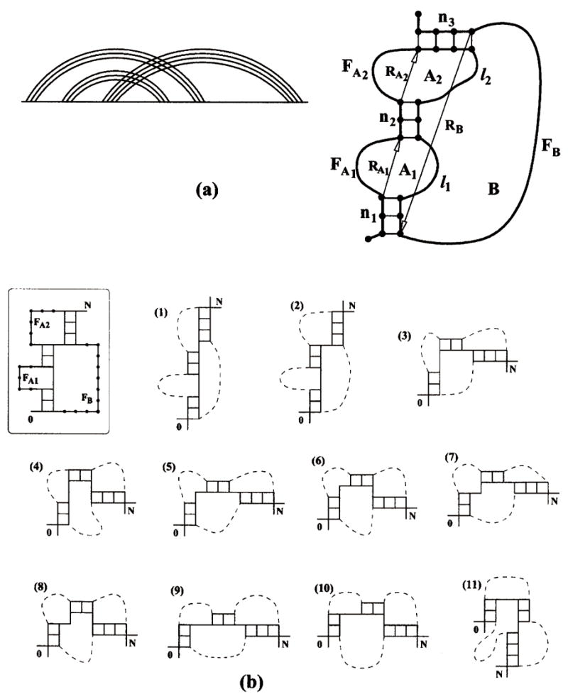
(a) The polymer graph and structure of a “pseudoknot” with an internal loop (A₁) formed in a helix stem. R_A1, R_A2, and R_B shown in the figure are the end-end vectors of the free loop segments F_A1, F_A2 and F_B, respectively. (b) The structure of the pseudoknot with three stems chosen to illustrate the method and the viable conformations of the enlarged interface. Two positions are shown for each of the end monomers 0 and N.

2. Generalized pseudoknots with three stems

As shown in Fig. 3, the enlarged interface for such a structure consists of three stems (n₁, n₂, n₃), two single-stranded interfacial segments (l₁, l₂), and two end monomers (0, N). For a given conformation I of the enlarged interface, the end-end vectors R_A1, R_A2, and R_B of the free loop segments F_A1, F_A2, and F_B, respectively, can be unambiguously determined. The conformational count of the pseudoknot in Fig. 3 can be calculated from the following sum over all the possible conformations I of the enlarged interface:

$${\mathrm{\Omega }}_P\simeq \sum _{\mathbf{I}}{\mathrm{\Omega }}_f({\mathbf{R}}_{A_1},f_{A_1})·{\mathrm{\Omega }}_f({\mathbf{R}}_{A_2},f_{A_2})·{\mathrm{\Omega }}_f({\mathbf{R}}_B,f_B).$$ (4)

3. Illustrative calculation for the number of conformations of pseudoknots with three stems

In Fig. 3(b), we show the structure of a pseudoknot with an internal loop formed in one of the helix stems so the pseudoknot is partially folded (unfolded) and contains three helix stems. Also shown in the figure are all the 11 viable conformations of the enlarged interface numbered from 1 to 11 (excluding the end monomers 0 and N). Since monomers 0 and N each can have two possible positions, from Eq. (4), we calculate the number of pseudoknot conformations as the following:

$${\mathrm{\Omega }}_P\simeq (2\times 2)\sum _{\mathbf{K}=1}^{11}{\mathrm{\Omega }}_f({\mathbf{R}}_{A_1},f_{A_1})·{\mathrm{\Omega }}_f({\mathbf{R}}_{A_2},f_{A_2})·{\mathrm{\Omega }}_f({\mathbf{R}}_B,f_B),$$ (5)

where K denotes an interface conformation shown in Fig. 3(b). The lengths of the free loop segments for the given pseudoknot are f_A1 = 5 for F_A1, f_A2 = 6 for F_A2, and f_B = 11 for F_B. The details of calculations are given in Table I, where we show, for each interfacial conformation K, the coordinates (x, y) of the end-end vectors and the approximate numbers of conformations Ω_f for each free loop segment (F_A1, F_A2, and F_B).

TABLE I.

Illustrative calculations for the number of conformations for a partially folded pseudoknot shown in Fig. 3(b).

K	(xA1, yA1)	${\mathrm{\Omega }}_f^{A_1}$	(xA2, yA2)	${\mathrm{\Omega }}_f^{A_2}$	(xB, yB)	${\mathrm{\Omega }}_f^B$	${\mathrm{\Omega }}_f^{A_1}·{\mathrm{\Omega }}_f^{A_2}·{\mathrm{\Omega }}_f^B$
1	(0,2)	1.0	(1,4)	2.6	(1, 7)	23.2	60.3
2	(0,2)	1.0	(2,3)	3.0	(2,6)	55.5	166.5
3	(1,3)	1.8	(1,4)	2.6	(−3, 3)	21.6	101.1
4	(1,3)	1.8	(2,3)	3.0	(−2, 2)	8.0	43.2
5	(2,2)	1.1	(1,4)	2.6	(−2, 4)	32.1	91.8
6	(2,2)	1.1	(2,3)	3.0	(−1, 3)	17.0	56.1
7	(2,2)	1.1	(1,4)	2.6	(−2, 4)	32.1	91.8
8	(2,2)	1.1	(2,3)	3.0	(−1, 3)	17.0	56.1
9	(3,1)	0.5	(1,4)	2.6	(−1, 5)	52.5	68.2
10	(3,1)	0.5	(2,3)	3.0	(0,4)	37.3	55.9
11	(4,0)	0.0	(1,4)	2.6	(−1, 1)	0.0	0.0
							Sum= 791.1

As shown in Table I, Eq. (5) gives ${\mathrm{\Omega }}_P^{\text{appr}}=4\times 791.1=3164.4$, which is close to the result from the exact computer enumeration: ${\mathrm{\Omega }}_P^{\text{exact}}=2799$.

IV. THERMAL UNFOLDING OF PSEUDOKNOTS

Central to the folding thermodynamics is the partition function. The calculation of partition function [Eq. (2)] for a given nucleotide sequence requires the enumeration of all the possible polymer graphs and the counting of conformations accessible to each graph. In the present study, we consider the complete ensemble of pseudoknotted structures as well as the secondary structures. For the secondary structure partition function, we use a previously developed statistical mechanical theory.^10,11

For the pseudoknotted conformations, in the preceding sections, we ignored the full tails and took into account only the first monomer of each tail closest to the pseudoknot structure element to represent the volume exclusion effect. We now add the full tails back to the calculation.

To take into account tails, we have used precalculated¹¹ tables for the numbers of tail conformations Ω_T(t) for tail length t≤ 24 and the following fitted formula for longer tails:¹¹

$$ln{\mathrm{\Omega }}_T(t)\simeq -2.62208+0.83927t+0.30984ln(t).$$

This formula has also been used to obtain the number of conformations of the open (fully unfolded) chain. With the conformational count of the tails, we can calculate the number of conformations of the pseudoknot with tails as the product of the number of conformations of the pseudoknot structure element Ω_P and the numbers of conformations of tails: Ω= Ω_PΩ_T(t₁)Ω_T(t₂), where t₁ and t₂ are lengths of the two tails at the 5′ and the 3′ terminals, respectively.

A. The Go-model pseudoknots

We consider a 33-mer chain with a fully folded native state shown in Fig. 4(a). As a simplified (Go-type) model, we assume that no other contacts besides those (native contacts) depicted in Fig. 4(a) can form. The interaction energy of each base pair stack is assigned to be −3 or −1 as shown in the figure. The energy of an isolated (unstacked) base pair is assumed to be 0.

FIG. 4.

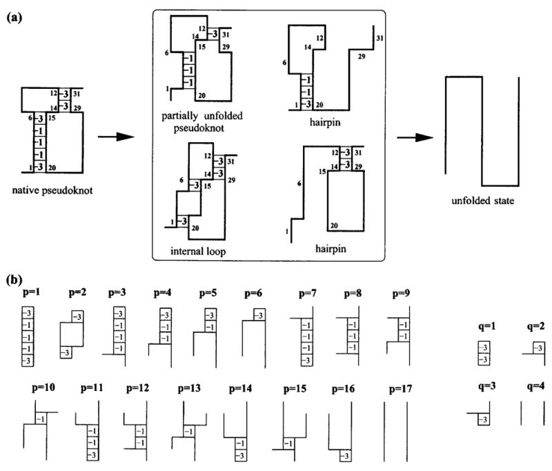
(a) The 33-mer pseudoknot-forming chain is used to illustrate the calculations for the density of states and partition function. The numbers in boxes (stacks) denote the energies of the corresponding (native) base stack. The four types of the representative partially unfolded conformations considered in the partition function calculation are shown. (b) The partially unzipped states of the (two) helix stems are labeled with parameters p and q, respectively. As a result, each state (folded, partially folded, and unfolded) can be represented by the parameter pair (p, q).

Since in the Go model, only the native contacts can form or disrupt in the folding/unfolding process, the conformational ensemble can be generated from the different ways to break the native contacts. Examples of partially unfolded states are also shown in Fig. 4(a). The unzipping of either helix stem can occur at the top, bottom, or internal base pair of the stem. The partially unfolded states of the pseudoknot can be conveniently represented by two parameters: p denotes the state of stem 1 and q of stem 2. The partially unfolded states of a stem depend on the stem length and can be enumerated. The possible states of stems of our native pseudoknot (five- and two-base stack) are shown in Fig. 4(b). In this way, each possible pseudoknot state can be described by a pair of numbers (p, q), which defines the set of contacts. For example, (p, q) = (1, 1) is the native pseudoknot in Fig. 4(a), (2,4) is a hairpin with an internal loop and (2,3) is a pseudoknot with an internal loop in stem 1.

The parameters p and q are used as the labels for the states of the stems. Each (p, q) pair unambiguously defines a pseudoknotted structure. The p’s and q’s shown in Fig. 4 are exhaustive for the short stems shown in the figure. As a caveat, we note that for illustrative purposes, we here use the two-dimensional lattice model, which excludes some conformations due to the lattice constraint (e.g., a 6-mer loop is not possible in a two-dimensional square lattice). In addition, in this section, in order to focus on the stem-loop interplay, we use the Go model, which disallows the formation of the misfolded states. For longer stems, more complex multiple internal loops can be formed. In the next section, we will go beyond the Go model by using the complete conformational ensemble, including all the possible misfolded structures.

To test the accuracy of the theory, we compute the density of states for all the possible pseudoknots (including all the partially unfolded states) and for the complete (pseudoknot/hairpin/open chain) conformational ensemble (including all the possible partially unfolded states) using both the theory developed here and the exact computer enumeration. Figure 5 shows the test results. We find good accuracy of the theoretical prediction.

FIG. 5.

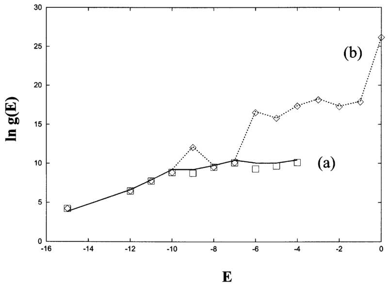
Test of the theory (line) against exact computer enumeration (symbols) for the density of states (a) for all the pseudoknotted conformations and (b) for the complete pseudoknot/hairpin/open conformational ensemble for the 33-mer chain shown in Fig. 4(a).

To study the folding thermodynamics for the model pseudoknot in Fig. 4(a), we calculate the free energy landscape F(p, q), which is the free energy of the macrostate for all the possible secondary structures and pseudoknots described by the conformational state (p, q). F(p, q) is computed from the following equation:

$$F(p,q)=E(p,q)-k_{B}Tln\mathrm{\Omega }(p,q),$$

where E(p, q) and Ω(p, q) are the energy (sum of the energies of the stacks) and the number of conformations of the macrostate described by (p, q). The free energy minima correspond to stable states. F(p, q) is temperature T dependent, and temperature change causes the change in the free energy landscape F(p, q) and the transitions between different stable states.

Figure 6(a) shows the free energy landscape F(p, q) for the model pseudoknot in Fig. 4(a). The landscape shows single pronounced minimum at (p, q) = (1, 1) [= the native state shown in Fig. 4(a)] at low temperature and (17,4) (= fully unfolded state) at high temperature. At k_BT = 0.672, the landscape shows that the transition between the native state and the unfolded state involves two hairpin conformations as the intermediate states: (17,1) and (1,4). Each hairpin intermediate is formed through the disruption of a helix stem of the native pseudoknot.

FIG. 6.

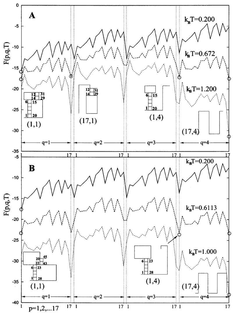
The free energy F(p, q, T) as a function of structure denoted by parameter pair (p, q). Free energy minima, i.e., stable states for a given temperature, are circled, and the representative conformations shown. (A) For the pseudoknot with smaller loops, the two hairpins (17, 1) and (1, 4), each formed through the disruption of a native helix stem, emerge as stable intermediate states. (B) For the pseudoknot with larger loops, the transition is three state: the native state, open chain, and hairpin with the longer helix stem, which are equally populated at k_BT = 0.6113.

In order to examine the competition between the helix and loop stability, we further calculate the free energy landscape for pseudoknots with different sizes of loops. For larger loops, as shown in Fig. 6(b), the free energy landscape reveals three-state transitions, where the native state, the open chain, and the hairpin with the longer stem are equally populated at k_BT = 0.6113. The larger loop would destabilize the folded state. As a result, state (17,1), which emerges as a folding intermediate for pseudoknot with smaller loops, is now absent. This is because the two-stack short helix stem in the (17,1) state is not stable enough to compete with the destabilizing larger loop. In contrast, the state (1,4) emerges as an intermediate because the five-stack long helix stem is sufficient enough to compete with (the larger) loop.

B. Pseudoknot folding with misfolded states

The formation of non-native contacts is not allowed in the above Go-model pseudoknots and therefore many structures, namely, the misfolded states, are excluded from consideration. In this section, we treat complete conformational ensemble, including all the possible misfolded conformations. We choose two (30- and 34-nt) pseudoknot-forming nucleotide sequences. We allow the formation of all the possible A–U and C–G base pairs. The energy of a base stack is equal to −1 for a stack formed by two A–U base pairs, −3 for a stack formed by one A–U and one C–G base pair, and −4 for a stack formed by two C–G pairs.

We enumerate all the possible secondary structures and pseudoknotted structures through the enumeration of all the possible polymer graphs. For each graph, we compute the energy E and the number of accessible conformations Ω. In Figs. 7 and 8 we show the free energy landscapes (F= E −k_BT ln Ω) for the 30-nt and the 34-nt sequences, respectively. The free energy landscapes show contrasting folding thermodynamics for the two sequences. The sequence in Fig. 7 unfolds through the sequential disruption of the two helix stems. The landscape at k_BT = 1.0 shows the emergence of an intermediate state (= minimum in the free energy landscape) which is formed through the breaking of the less stable two-stack helix in the native pseudoknot. In contrast, the sequence in Fig. 8 unfolds through the formation of a misfolded state I, shown as the minimum in the free energy landscape at k_BT = 0.9. The misfolded intermediate (hairpin I in Fig. 8) is formed through a complete rearrangement of the base pairs from the native pseudoknot.

FIG. 7.

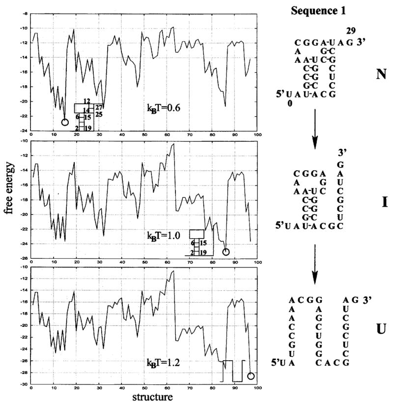
The free energy as a function of structure for a 30-mer nucleotide sequence. The unfolding is a two-step process with the (less stable) shorter helix stem disrupted first (N→I) followed by the breaking of the longer (more stable) helix stem (I→U).

FIG. 8.

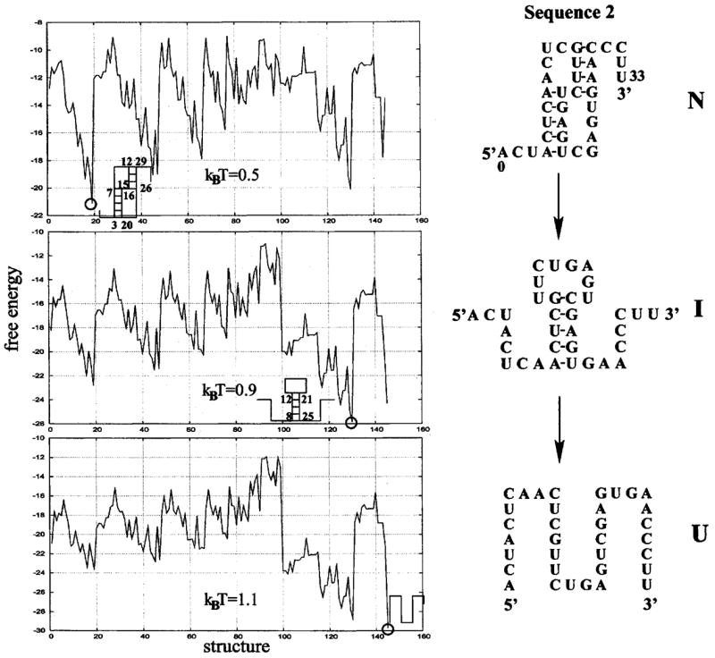
Free energy as a function of structure. The melting process for the 34-mer nucleotide sequence involves a misfolded hairpin (I) as an intermediate state.

V. MECHANICAL UNFOLDING OF PSEUDOKNOTS

In the mechanical unfolding experiments, a stretching force in the piconewton (pN) range generated by atomic force microscopy or laser or magnetic tweezers is applied to pull a biomolecule to unfold the molecule.^13–15 Such experiments have been conducted on proteins,^16–18 DNA,¹⁹ and RNA.^20–23 The advantage of the single-molecule experiments is the possibility to follow the individual folding-unfolding trajectory (which is difficult in bulk studies where multiple species and multiple folding pathways are present) and to stretch the molecule along the well-defined coordinates.

The mechanical unfolding experiments have inspired the theoretical studies on the force induced folding/unfolding of biomolecules.^24–27 One of the important features in the force induced unfolding is the dependence on the choice of the statistical ensemble, namely, which variables are held constant and which are allowed to fluctuate in the unfolding process. In the experiments where the molecule is stretched by force, the following two types of statistical ensembles are generally considered.

1. Constant distance ensemble (isometric): The molecule’s end-end distance is held constant, and the fluctuation of the force is recorded in experiment. Such an experiment can be performed, for example, in the following way. One end of the molecule can be attached to a rigid support, and the other end is attached to the bead held in optical trap. The feedback loop controls the position of the trapped bead with respect to the other end of the molecule and cancels its fluctuations by moving the trap center. The fluctuating force, which is proportional to the displacement of the bead in the optical trap from its equilibrium position, as a function of time can be determined from the movement of the optical trap. In the equilibrium unfolding process, the molecule’s end-end distance (extension) D is changed slowly, and the mean force averaged over the appropriate time period F̄ as a function of D is plotted as the force-extension curve.

2. Constant force ensemble (isotensional): The force is held constant, and the molecule’s end-end distance fluctuates. In such experiments, the feedback loop makes the optical trap move in such a way that the bead position with respect to the center of the optical trap is fixed (which means that the fixed force is acting at the bead). The fluctuating end-end distance is then averaged and recorded as D̄(F). The equivalent force-extension curve F(D̄) can be obtained by the inversion of the relation D̄(F).

It was shown²⁸ that the difference between results of isometric and isotensional experiments is essential when the system is small (short molecules). For long and flexible molecules the fluctuations of variables are negligible and the difference between the two statistical ensembles vanishes.

Our RNA pseudoknot folding thermodynamics theory developed above can be further developed to study the thermodynamics of the mechanical unfolding of RNA pseudoknot. We assume that the two ends of the molecule are attached to two beads whose positions and the acting force are controlled by the force-extension measuring device. In our calculations, we consider the fixed force and fixed extension ensembles separately.

We assume that one end of the chain is fixed and the constant force f is applied to the other end in the constant force experiments. The average end-end vector D of the molecule is recorded as a function of f. The work f•D done on the molecule by force f contributes to the energy of the molecule, and the partition function for the constant force ensemble is

$$Z(T,\mathbf{f})=\sum _E\sum _{\mathbf{D}}g(E,\mathbf{D})e^{-(E-\mathbf{f}·\mathbf{D})/k_{B}T},$$ (6)

where g(E, D) is the constrained density of states, i.e., the number of conformations with the energy E and end-end vector D. From Z(T, f), the mean extension of the chain at the given force can be calculated as

$$\overline{\mathbf{D}}(T,\mathbf{f})=k_{B}T\frac{\partial }{\partial \mathbf{f}}lnZ(T,\mathbf{f}).$$ (7)

In the constant extension experiments, the end-end vector D of the chain is assumed to be held constant and the average force f acting on the molecule is recorded as a function of D. Since D is constant, the partition function for the constant extension ensemble is

$$Z(T,\mathbf{D})=\sum _{E}g(E,\mathbf{D})e^{-E/k_{B}T}.$$ (8)

If Z(T, D) is known, the mean force f̄ corresponding to the given D can be calculated by the formula

$$\overline{\mathbf{f}}(T,\mathbf{D})=-k_{B}T\frac{\partial }{\partial \mathbf{D}}lnZ(T,\mathbf{D}).$$ (9)

A. Density of states

In both the constant force and constant extension models, the key problem is how to calculate the density of states g(E, D), which is the total number of conformations with energy E and end-end vector D. We assume that one end of the molecule is attached to the wall and the force f acting on the molecule is directed perpendicular to the wall. Instead of the end-end vector D, we consider its component denoted as D, in the direction of the force. In the partition function calculation, the conformational ensemble includes both secondary structures and pseudoknotted structures. To find the number of conformations with a tail attached to the wall and the end of the other tail being at the distance D from the wall, we use the following approach. The structure can be divided into three parts: two tails and the structure element. For a given D, we exhaustively enumerate all the possibilities of three numbers: D₁ (= extension of tail 1), D_P (= end-end extension of the structure element), and D₂ (= extension of tail 2), such that D₁ + D_P + D₂ = D. For each set of (D₁, D_p, D₂), we calculate the product of the numbers of conformations of the first tail with extension D₁, of the structure element with extension D_P, and of the second tail with extension D₂. In what follows we give detailed description for the calculation for pseudoknotted and secondary structures, separately.

1. Pseudoknotted conformations

To illustrate the principle, we choose the 2D lattice representation for chain conformations. On the two-dimensional lattice, a pseudoknot structure element (without tails) can have four different orientations with respect to the wall (Fig. 9). Since we consider the pseudoknot to be the central part of the structure, a convenient choice of the coordinate system (x, y) would be such that the y axis is along the stem with the tail attached to the wall. This is the same coordinate system as the one used for the calculation of the number of pseudoknot conformations (Fig. 1, Sec. III). In such coordinate system, the wall and the force have different orientations with respect to the pseudoknot (Fig. 9).

FIG. 9.

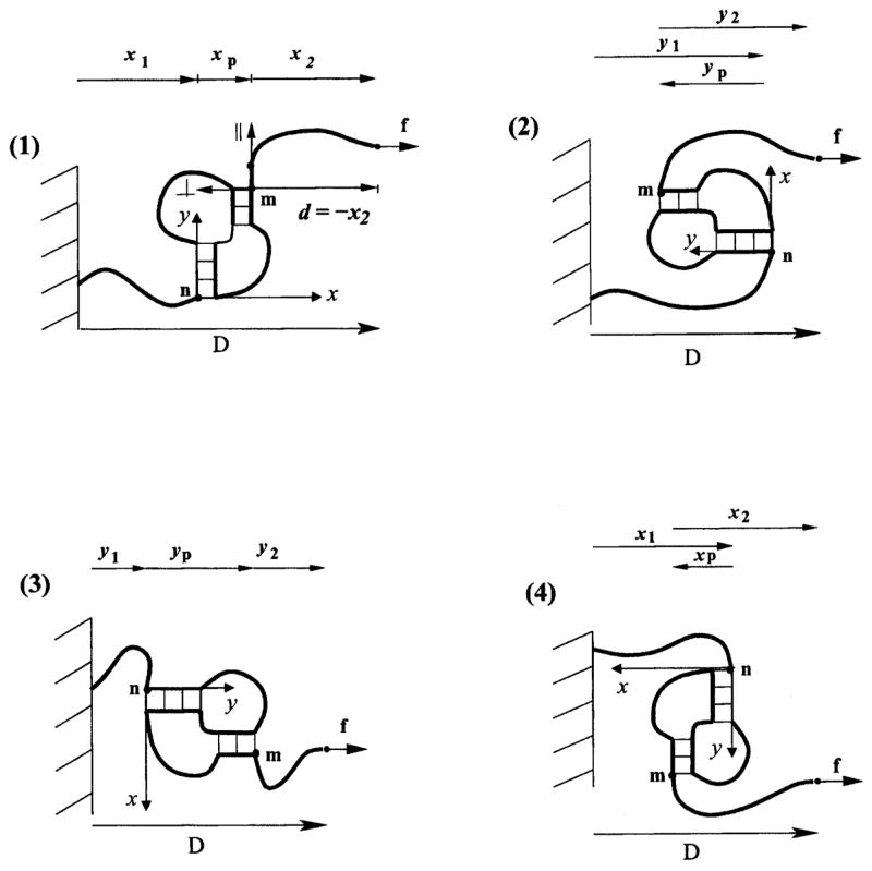
In the two-dimensional lattice model, a pseudoknot can have four possible orientations with respect to the wall. x_p = x(m) −x(n) and y_p = y(m) −y(n). The coordinate system can be defined by the position of the first stem of the pseudoknot (y axis along the stem), while the || and ⊥ axes of the tail is defined by the orientation of the first bond as shown in (1).

For a fixed orientation of the pseudoknot, we need two different functions for the conformational count of tails: ${\mathrm{\Omega }}_T^{\parallel }(t,d)$ and ${\mathrm{\Omega }}_T^{\perp }(t,d)$, which denote the numbers of conformations for a tail of length t with end-end distance d in the direction parallel (||) and perpendicular (⊥) to the first (closest to the pseudoknot structure element) bond of the tail, respectively. We have obtained the ${\mathrm{\Omega }}_T^{\parallel }$ and ${\mathrm{\Omega }}_T^{\perp }$ functions by means of exact computer enumeration for 1 ≤ t ≤ 11.

For a given extension D along the line of the action of force, we follow the following procedure to calculate the density of states (the number of conformations) for the pseudoknots.

1. We enumerate the different orientations of the pseudoknot, as shown in Fig. 9.

2. For each pseudoknot orientation, we enumerate the conformations of the pseudoknot enlarged interface. For a given enlarged interface conformation, the two helix stems, the energy E of the pseudoknot, and the end-end vector (x_p and y_p in Fig. 9) and the extension D_P of the pseudoknot element are all fixed.

3. For each enlarged interface conformation, using Eq. (3), we calculate the number of pseudoknot conformations Ω_P.

4. We enumerate all the possibilities of D₁ and D₂ such that D₁ + D₂ = D − D_P. The numbers of tail 1 and tail 2 conformations which correspond to the given D₁ and D₂, respectively, are approximated by the function ${\mathrm{\Omega }}_T^{\parallel }(t,d)$ or ${\mathrm{\Omega }}_T^{\perp }(t,d)$. Which of two Ω_T functions should be used depends on the orientations of the wall and the force with respect to the pseudoknot (cases 1–4 in Fig. 9) and on the directions of the first bonds of the tails. For example, for the first bond of tail 2 directed upward in Fig. 9 case 1, the number of tail 2 conformations which have the end-end extension D₂ along the x axis, equals ${\mathrm{\Omega }}_T^{\perp }(t_2,d=-x_2)$, because tail 2 has the end-end extension d = −D₂ = −x₂ along the tail’s (local) ⊥ axis (see Fig. 9).

5. For each pair of (D₁, D₂), we calculate the product of the number of conformations Ω_P of the pseudoknot with the given enlarged interface and the numbers of conformations of the tails ${\mathrm{\Omega }}_T^z(t_1,d_1)$ and ${\mathrm{\Omega }}_T^z(t_2,d_2)$, where t₁ and t₂ are the lengths of the two tails, z = || or ⊥, and d₁ and d₂ are required extensions of tails in direction z.

6. The density of states g_P(E, D) for pseudoknotted structures with energy E and end-end distance D is given by the sum over (i) all the possible (D₁, D₂), (ii) the enlarged interface conformations I, and (iii) the pseudoknot orientations,

   $$g_P(E,D)=\sum _{\text{orientation}}\sum _{\mathbf{I}}\sum _{D_1}\sum _{D_2}{\mathrm{\Omega }}_T(t_1,d_1)·{\mathrm{\Omega }}_P·{\mathrm{\Omega }}_T(t_2,d_2).$$ (10)

   Here the value of parameters d₁ and d₂ are determined by the orientation of the pseudoknot with respect to the wall and by the enlarged interface conformation I, which defines the direction of the first tail bonds with respect to the pseudoknot.

For the number of conformations Ω_T for the single-stranded chain segments, we have exactly enumerated the conformations for different chain lengths 10≤ l ≤ 28 and different extensions D ≤ l. We find that we can fit the results by two different functions:

$$\begin{array}{l}ln{\mathrm{\Omega }}_T(l,D)=(-2.34782+0.803224l)\\ +(-0.0239763+2.59832/l)D\end{array}$$ (11)

for D ≤ l/2 (less stretched chain) and

$$ln{\mathrm{\Omega }}_T(l,D)=\left[\frac{3.1649436}{l}-\frac{4.19464}{l^2}\right]D(l-D)$$ (12)

for l/2 ≤ D ≤ l (more stretched chain). In Fig. 10(c), we show the comparison between the above approximated Ω_T(l, D) and that from exact computer enumeration and find good agreement. The above approximations for ln Ω_T(l, D) are used as extrapolations for longer open chains.

FIG. 10.

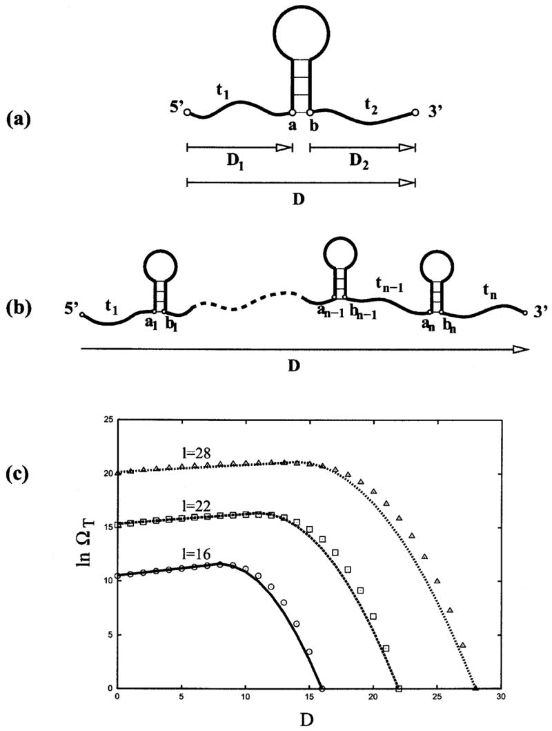
(a) A hairpin (with tails) can be divided into hairpin element and the single-stranded segment, which consists of two tails (t₁ and t₂) and the outermost contact (a, b) of the hairpin structure element. (b) A general secondary structure can be decomposed as multiple sequentially connected secondary structure elements. (c) The number of conformations of a single-stranded segment as a function of the segment’s length l and the end-end extension D from exact enumeration (symbols) and the analytical approximation (lines).

2. Secondary structures

We first use hairpin conformations to illustrate the methodology. We will then generalize the theory to treat more complex secondary structures. A unique feature of a hairpin structure element with tails is that the end-end distance (between monomers a and b in Fig. 10) is fixed. So the conformational count for a given total extension D can be calculated as

$$g_2(E,D)\simeq k{\mathrm{\Omega }}_H(E)·{\mathrm{\Omega }}_T(l,D),$$ (13)

where Ω_H(E) is the number of conformations of the hairpin element (from a to b without tails) with energy E, Ω_T(l, D) is the number of conformations of the single-stranded chain segment as a function of length l = t₁ + t₂ + 1 and the extension D [see Fig. 10(a)], and the prefactor k accounts for the volume exclusion between the tails and the hairpin structure element. We find that k ≃ 1/4 for D ≤ l −4 and k ≃ 1 otherwise.

For secondary structures, which consist of multiple sequentially connected secondary structure elements (e.g., hairpins), we calculate the density of states from the following recursive relation [see Fig. 10(b)]:

$$g_2^{(n)}(E,D)=k{\mathrm{\Omega }}_H^{(n)}(E_n)g_2^{(n-1)}(E-E_n,D),$$ (14)

where $E={\mathrm{\Sigma }}_{i=1}^n{E}_i$ is the total energy, E_i is the energy of the ith secondary structure element (between a_i and b_i), and $g_2^{(n-1)}$ is the density of states of a reduced chain, where the nth structure element (between a_n and b_n) is replaced by a single bond connecting a_n and b_n. ${\mathrm{\Omega }}_H^{(n)}(E_n)$ is the number of conformations of the nth secondary structure element.

The sum of the densities of states for secondary and pseudoknot structures gives the (total) density of states g(E, D) in Eqs. (6) and (7). In Fig. 11, we show the tests for our theory against exact computer enumeration for a 38-mer pseudoknot-forming chain. We find good agreements.

FIG. 11.

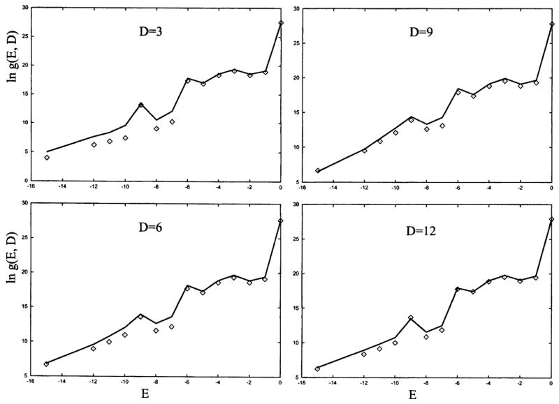
The density of states g(E, D) for the pseudoknot/hairpin/open chain conformational ensemble for the 38-mer pseudoknot [shown in Fig. 4(a) with added tails of lengths t₁ = 3 and t₂ = 4]. Symbols: from exact enumeration; lines: from the theory developed in this study.

B. Force-extension curve, misfolded pseudoknots, and folding thermodynamics

We consider two specific pseudoknot-forming nucleotide sequences for which thermal unfolding processes have been studied (Figs. 7 and 8). In the calculation for the density of states, we enumerate all the possible secondary and pseudoknotted states, including all the possible misfolded states and partially folded states. We show the predicted force-extension curves and the conformational changes for the two sequences in Fig. 12.

FIG. 12.

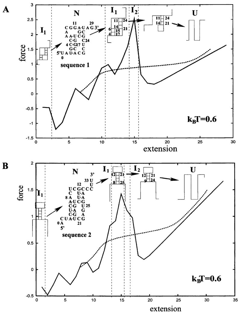
The calculated isometric (solid lines) and the isotensional (dashed lines) force-extension curves and the structural transitions for the two nucleotide sequences specified. For both sequences, the misfolded structures (I₁) emerges as intermediate states for those extensions of the molecules at which the overstretched native pseudoknots are less stable.

We find that for the two sequences, both the isometric and isotensional curves show a major transition from the native pseudoknot (N) to a misfolded intermediate state (I₁). A notable feature shown in Fig. 12 is that the misfolded intermediate (I₁) emerges when the extension of the molecule is both small and large compared to the average extension of the native pseudoknot N. The formation and the reformation of the intermediate state I₁ (with both small and large extensions) can be explained in the following way.

The native pseudoknots have shorter tails than the intermediate states. Therefore, the end-end extension of the native pseudoknot is much more restricted than that of the intermediate state I₁. For instance, for sequence 1 in Fig. 12(a), the end-end extension for the native pseudoknot N and the intermediate I₁ in a two-dimensional lattice are in the ranges of [3, 10] and [1, 13], respectively. Therefore, for sequence 1, for extension outside the range of [3,10], the native pseudoknot cannot exist and new structure would emerge. In contrast, the intermediate state I₁ can accommodate a wide range of extension and can exist as a stable state outside the range of [3,10].

As shown in Fig. 10(c), the number of tail conformations quickly decreases as the tail is stretched. When the native pseudoknot, which has short tails, is restricted to have very small or large extensions, the tails would inevitably be stretched. The entropy of the tails is small and the free energy F = E −TS of the structure is high. Therefore, the native pseudoknot is unstable and a structural transition would occur. For the misfolded structures (I₁), however, the longer tails allow the chains to achieve the required (small or large) extensions without becoming highly stretched. So the intermediate state can be more stable than the native pseudoknots for small and large extensions.

In the limiting regime of very small end-end extension, the chain is in highly compact (and thus low-entropy) states. Large extension would cause an increase in the freedom of such highly compressed chain. So in the small extension limit, larger extension would lead to lower free energy, resulting in an apparent negative equilibrium pulling force.

Another notable feature in Fig. 12 is that sequence 1 mechanically unfolds through very different steps of conformational transitions than thermal unfolding. The thermal unfolding involves simple disruptions of native contacts, while in the mechanical unfolding, the native pseudoknot unfolds, refolds, and unfolds again during the pulling process. In contrast, for sequence 2, the intermediate state is the same misfolded hairpin as that in the thermal unfolding.

VI. CONCLUSION AND DISCUSSION

We present a statistical mechanical theory for the folding thermodynamics of pseudoknotted chain conformations, including all the possible partially folded and misfolded structures. The model enables the calculation of conformational entropy and the partition function of pseudoknots. The key idea of the theory is (i) to decompose a pseudoknot structure into stem-loop subunits, (ii) to separate out the interfacial segments between the subunits, and (iii) to account for the correlation and volume exclusion between subunits through localized effects within and near the interface. The theory has been shown to give good predictions for the folding thermodynamics as tested against exact computer enumerations. The theory enables predictions for the folding stability, nativelike and misfolded folding intermediates, and folding free energy landscapes for pseudoknotted and secondary structures.

The current form of the model is not without limitations. Possible further development of the model should address the following issues.

1. More realistic off-lattice chain representations can be used within the present graph-theoretic framework. An example of the possible off-lattice representation is the virtual bond model,^29,30 where the six bonds of each nucleotide backbone are replaced by two virtual bonds. The length of the virtual bond is nearly fixed (3.9 Å),³⁰ and the conformation of each nucleotide is described by the torsional angles of the virtual bonds.

2. Noncanonical intraloop interactions and other tertiary interactions can play important roles in the sequence and temperature dependence of the loop entropy and the folding thermodynamics and therefore should be taken into account in the further development of the model. The generality of the basic ideas in the current model suggests the possibility to systematically extend the model to treat more complex tertiary folds, including ones with multiple crossing-linked contacts.⁸

3. The helical stems in pseudoknots tend to form the energetically favorable coaxial stacks. Such coaxial stacking is neglected in the present model and should be included in the further development of the model.

4. RNA folding is strongly dependent on the ionic solution condition. To properly take into account this effect, the chain conformational model should be combined with the polyelectrolyte theory to account for the ion electrostatics.

Thermodynamic parameters (especially the conformational entropy) for pseudoknotted structures are currently very limited, mainly due to the lack of a rigorous statistical mechanical model for pseudoknot folding. The present model provides a general method for the computation of the conformational entropy for pseudoknots. Moreover, the statistical mechanical framework developed here can also be used to extract the thermodynamic parameters from the experiments.

References

- 1.Turner DH, Sugimoto N, Freier SM. Annu Rev Biophys Biophys Chem. 1988;17:167. doi: 10.1146/annurev.bb.17.060188.001123. [DOI] [PubMed] [Google Scholar]
- 2.Freier SM, et al. Proc Natl Acad Sci USA. 1986;83:9373. doi: 10.1073/pnas.83.24.9373. [DOI] [PMC free article] [PubMed] [Google Scholar]
- 3.Jaeger JA, Turner DH, Zuker M. Proc Natl Acad Sci USA. 1989;86:7706. doi: 10.1073/pnas.86.20.7706. [DOI] [PMC free article] [PubMed] [Google Scholar]
- 4.Gultyaev AP, van Batenburg FHD, Pleij CWA. RNA. 1999;5:609. doi: 10.1017/s135583829998189x. [DOI] [PMC free article] [PubMed] [Google Scholar]
- 5.Jacobson H, Stockmayer WH. J Chem Phys. 1950;18:1600. [Google Scholar]
- 6.Abrahams JP, van den Berg M, van Batenburg E, Pleij C. Nucleic Acids Res. 1990;18:3035. doi: 10.1093/nar/18.10.3035. [DOI] [PMC free article] [PubMed] [Google Scholar]
- 7.Lucas A, Dill KA. J Chem Phys. 2003;119:2414. [Google Scholar]
- 8.Kopeikin Z, Chen SJ. J Chem Phys. 2005;122:094909. doi: 10.1063/1.1857831. [DOI] [PMC free article] [PubMed] [Google Scholar]
- 9.Fiebig KM, Dill KA. J Chem Phys. 1993;98:3475. [Google Scholar]
- 10.Chen SJ, Dill KA. J Chem Phys. 1995;103:5802. [Google Scholar]
- 11.Chen SJ, Dill KA. J Chem Phys. 1998;114:4602. [Google Scholar]
- 12.Zhang W, Chen SJ. J Chem Phys. 2001;114:7669. [Google Scholar]
- 13.Tinoco I., Jr Annu Rev Biophys Biomol Struct. 2004;33:363. doi: 10.1146/annurev.biophys.33.110502.140418. [DOI] [PMC free article] [PubMed] [Google Scholar]
- 14.Zhuang X, Rief M. Curr Opin Struct Biol. 2003;13:88. doi: 10.1016/s0959-440x(03)00011-3. [DOI] [PubMed] [Google Scholar]
- 15.Bustamante C, Smith SB, Liphardt J, Smith D. Curr Opin Struct Biol. 2000;10:279. doi: 10.1016/s0959-440x(00)00085-3. [DOI] [PubMed] [Google Scholar]
- 16.Carrion-Vazquez M, Oberhauser AF, Fisher TE, Marszalek PE, Li H, Fernandez JM. Prog Biophys Mol Biol. 2000;74:63. doi: 10.1016/s0079-6107(00)00017-1. [DOI] [PubMed] [Google Scholar]
- 17.Kellermayer MS, Smith SB, Granzier HL, Bustamante C. Science. 1997;276:1112. doi: 10.1126/science.276.5315.1112. [DOI] [PubMed] [Google Scholar]
- 18.Tskhovrebova L, Trinick J, Sleep JA, Simmons RM. Nature (London) 1997;387:308. doi: 10.1038/387308a0. [DOI] [PubMed] [Google Scholar]
- 19.Bockelmann U, Thomen P, Essevaz-Roulet B, Viasnoff V, Heslot F. Biophys J. 2002;82:1537. doi: 10.1016/S0006-3495(02)75506-9. [DOI] [PMC free article] [PubMed] [Google Scholar]
- 20.Liphardt J, Onoa B, Smith SB, Tinoco I, Jr, Bustamante C. Science. 2001;292:733. doi: 10.1126/science.1058498. [DOI] [PubMed] [Google Scholar]
- 21.Liphardt J, Dumont S, Smith SB, Tinoco I, Jr, Bustamante C. Science. 2002;296:1832. doi: 10.1126/science.1071152. [DOI] [PubMed] [Google Scholar]
- 22.Onoa B, Dumont S, Liphardt J, Smith SB, Tinoco I, Jr, Bustamante C. Science. 2002;299:1892. doi: 10.1126/science.1081338. [DOI] [PMC free article] [PubMed] [Google Scholar]
- 23.Harlepp S, Marchal T, Robert J, Leger JF, Xayaphoumimine A, Isambert H, Chatenay D. Eur Phys J E. 2003;12:605. doi: 10.1140/epje/e2004-00033-4. [DOI] [PubMed] [Google Scholar]
- 24.Cocco S, Monasson R, Marko JF. Proc Natl Acad Sci USA. 2001;98:8608. doi: 10.1073/pnas.151257598. [DOI] [PMC free article] [PubMed] [Google Scholar]
- 25.Montanari A, Mezard M. Phys Rev Lett. 2001;86:2178. doi: 10.1103/PhysRevLett.86.2178. [DOI] [PubMed] [Google Scholar]
- 26.Gerland U, Bundschuh R, Hwa T. Biophys J. 2001;81:1324. doi: 10.1016/S0006-3495(01)75789-X. [DOI] [PMC free article] [PubMed] [Google Scholar]
- 27.Gerland U, Bundschuh R, Hwa T. Biophys J. 2003;84:2831. doi: 10.1016/S0006-3495(03)70012-5. [DOI] [PMC free article] [PubMed] [Google Scholar]
- 28.Keller D, Swigon D, Bustamante C. Biophys J. 2003;84:733. doi: 10.1016/S0006-3495(03)74892-9. [DOI] [PMC free article] [PubMed] [Google Scholar]
- 29.Olson WK. Macromolecules. 1980;13:721. [Google Scholar]
- 30.Cao S, Chen SJ. RNA. 2005;11:1884. doi: 10.1261/rna.2109105. [DOI] [PMC free article] [PubMed] [Google Scholar]