Detection of protein fold similarity based on correlation of amino acid properties

Abstract

An increasing number of proteins with weak sequence similarity have been found to assume similar three-dimensional fold and often have similar or related biochemical or biophysical functions. We propose a method for detecting the fold similarity between two proteins with low sequence similarity based on their amino acid properties alone. The method, the proximity correlation matrix (PCM) method, is built on the observation that the physical properties of neighboring amino acid residues in sequence at structurally equivalent positions of two proteins of similar fold are often correlated even when amino acid sequences are different. The hydrophobicity is shown to be the most strongly correlated property for all protein fold classes. The PCM method was tested on 420 proteins belonging to 64 different known folds, each having at least three proteins with little sequence similarity. The method was able to detect fold similarities for 40% of the 420 sequences. Compared with sequence comparison and several fold-recognition methods, the method demonstrates good performance in detecting fold similarities among the proteins with low sequence identity. Applied to the complete genome of Methanococcus jannaschii, the method recognized the folds for 22 hypothetical proteins.

The tremendous explosion in the amount of genome sequences during the past few years makes functional characterization of gene products overwhelming. The most common way of inferring the function of a new gene is based on sequence similarity with proteins of known function. Classical sequence comparison algorithms like ssearch (1), fasta (2), or blast (3) were designed to assess the degree of sequence similarities between compared sequences. However, an increasing number of proteins with weak sequence similarity has been found to assume similar three-dimensional (3D) folds, referred here as remote homologues, and often have similar or related biochemical or biophysical functions. (In this work remote homologues imply only structure similarity of proteins rather than their evolutionary relationship, because the latter is often difficult to establish reliably for strongly divergent sequences.) To detect such fold similarity a variety of 3D-threading methods have been developed; in these methods, amino acid sequence of a new protein is compared with the 3D amino acid profiles of proteins with known structures (4–8).

Because 3D-threading methods require the knowledge of the 3D structure of one of the two compared proteins, they are effective only for finding the remote homologues of the proteins with known 3D structures. To overcome this limitation, sequence alignment was combined with alignment of structural properties predicted or derived from sequence [one-dimensional (1D) threading]. The alignment of the predicted secondary structure only (9) or the predicted secondary structure and solvent accessibility of proteins (10) was shown to be useful for fold recognition. Adding sequence information by using a sequence similarity matrix works better (11–14), though finding the optimal matrix remains a challenge. The matrices currently available were derived from the statistics of known protein sequences or structures (11–16) and, thus, may be biased toward the current databases (17).

Because the three-dimensional structure of a protein is determined by the physical and chemical properties of all residues, we make a simplifying assumption that the local interactions in proximity of each residue in the protein are similar to those of the corresponding residue in its remote homologues. We make a further assumption that, because sequentially adjacent residues are usually proximal to each other in structure, the sequential arrangement of physical properties of amino acids flanking a given residue is likely to be correlated to that of the corresponding residue in remote homologues. This hypothesis is the basis of our method, the proximity correlation matrix (PCM) method, for detecting fold similarities between two protein sequences.

Detection of protein fold similarities has two major applications: (i) fold recognition, where a query sequence is compared with those of the proteins of known fold, and (ii) fold classification, where protein sequences are clustered into groups with the same predicted fold even when the fold information is not available. Here we present the results of the first application of the PCM method. The method is tested on a number of proteins with known structures and known remote homologues, compared with PSI-BLAST (18) and several 1D-threading techniques (11–15), and applied to the complete genome of Methanococcus jannaschii (19).

Algorithm

Data Sets.

For query proteins representing 64 folds (Table 1), we looked for their remote homologues in a target set composed of 1,390 protein sequences with sequence identity among them not exceeding 25% [nonredundant set of FSSP database (20)]. Using structural classification of proteins (SCOP) (21), we chose the 64 protein fold families, each including at least three remote homologues in the target set. Four hundred and twenty of 1,390 proteins in the target set belong to these fold families. Protein domains with fewer than 90 residues as well as the composite fold domains, i.e., consisting of more than one polypeptide chain or sequentially distant parts of the same chain, were eliminated.

Table 1.

The most-populated protein folds and their representative query proteins

Fold name	Class	N	Protein	L
5′ to 3′ exonuclease	α/β	3	1tfr	283
6-Bladed β-propeller	β	3	2sil	381
7-Bladed β-propeller	β	3	2bbkH	355
Acid proteases	β	5	1fmb	104
Actin-depolymerizing proteins	α + β	3	1svr	94
Adenine nucleotide α-hydrolase	α/β	5	1nsyA	271
Barrel-sandwich hybrid	β	5	1htp	131
Biotin carboxylase, N-term/ATP-grasp	Multi	3/6	1gsa	122/192
C2 domain-like	β	3	1rsy	135
Class II aaRS and biotin synthetases	α + β	6	1sesA	311
ConA-like lectins	β	7	1lcl	141
C-type lectin-like	α + β	6	1lit	129
Cupredoxins	β	8	1plc	99
Cyclin-like	α	3	1volA	95/109
Cystatin-like	α + β	7	1opy	123
Cysteine proteinases	α + β	3	1ppn	212
Cytochrome c	α	5	1cyj	90
Cytochrome P450	α	5	1phd	405
Double psi β-barrel	β	3	2eng	205
Double-stranded β-helix	β	6	1caxB	184
EF hand-like	α	11	1ncx	162
Enolase, N-term	α + β	3	2mnr	130
FAD/NAD(P)-binding domain	α/β	8	1trb	126
Ferredoxin-like	α + β	17	2ula	90
Ferritin-like	α	8	1bcfA	157
Flavodoxin-like	α/β	14	3chy	128
Fold of diphtheria toxin	β	6	1exg	110
Four-helical cytokines	α	11	1bgc	158
Four-helical up-and-down bundle	α	9	2ccyA	127
Galactose-binding domain-like	β	3	1ulo	152
Globin-like	α	12	2fal	146
Immunoglobulin-like β-sandwich	β	39	1tlk	103
Lipocalins	β	6	1mup	157
Lysozyme-like	α + β	4	1chkA	238
Methyltransferases	α/β	4	1vid	214
NAD(P)-binding Rossmann-fold domains	α/β	24	1eny	268
OB-fold	β	16	1prtF	98
Periplasmic-binding protein-like I	α/β	7	2dri	271
Periplasmic-binding protein-like II	α/β	8	1sbp	309
PH domain-like	β	7	1dynA	113
Phosphoribosyltransferases	α/β	4	1nulA	142
Phosphorylase/hydrolase-like	α/β	6	1xjo	271
P-loop containing NTP hydrolases	α/β	9	1hurA	180
PLP-dependent transferases	α/β	3	2dkb	431
Porins	TM	4	2por	301
Protein kinases	Multi	5	1csn	293
Reductase/ferredoxin reductase, C-term.	Multi	7/4	1fnc	136/160
Restriction endonucleases	α/β	5	1pvuA	154
Ribonuclease H-like motif	α/β	12	1itg	142
Single-stranded left-handed β-helix	β	3	1thjA	213
Sugar phosphatases	Multi	3	1imbA	272
The “swiveling” β/β/α-domain	α/β	3	1zymA	247
Thiamin-binding	α/β	3	1pvdA	180/196
Thioredoxin fold	α/β	9	1thx	108
Toxins’s membrane translocation domains	TM	5	1colA	197
Trypsin-like serine proteases	β	5	2sga	181
Viral coat and capsid proteins	β	17	1bbt1	186
Zincin-like	α + β	7	1kuh	132
α/β-hydrolases	α/β	12	1whtB	153
β/α (TIM)-barrel	α/β	46	1nar	289
β-clip	β	3	1dupA	136
β-Grasp	α + β	4	1put	106
β-Prism I	β	3	1vmoA	163
β-Trefoil	β	5	1hce	118

Fold name and Class are assigned according to SCOP classification (21), N is number of proteins (domains) in the given fold in the target set; Protein Database code and length of a representative protein are listed under Protein and L, respectively. In a multidomain protein, the lengths and fold names of domains are separated with a slash. 

Protein Representation.

Each amino acid residue in a protein is described in terms of two quantities: secondary structure conformation (helix, strand, or coil) and one of the five physical properties representing the five major clusters of amino acid indices summarized by Tomii and Kanehisa (22). They are hydrophobicity (23), volume (24), normalized frequencies of α-helix (25), normalized frequencies of β-sheet (25), and relative frequency of occurrence (26). Both real [assigned by DSSP (27)] and predicted [using program psipred by David Jones (28)] secondary structures are used for testing.

Proximity Correlation Matrix.

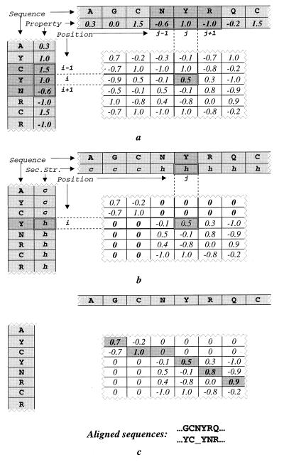
For an amino acid residue i we defined its proximity by a “window,” i.e., a short fragment of the protein sequence extended from position i to i − l in one direction and to i + l in the other. The size of the window, L = 2l + 1 (l = 1, 2, 3) is varied in different experiments. For two given fragments in the two sequences compared, each fragment represented by the middle position (i and j, respectively; see Fig. 1a), we defined the correlation of a physical property p as:

1

where p̄ⁱ and σⁱ are the average and SD, respectively, of the property in the fragment defined by the window centered at i.

Figure 1.

Construction of a proximity correlation matrix. In each panel, the segment of amino acid sequence of a query protein (using a one-letter code) and the corresponding vector of properties are shown vertically. Those of a target protein are shown horizontally. (a) First, the coefficient of correlation (Eq. 1) of a given physical property [e.g., hydrophobicity (23)] between two short sequence fragments (i − 1, i + 1) and (j − 1, j + 1) of two proteins is assigned to the matrix element (i, j). (b) Second, all matrix elements (i, j) where secondary structure conformations (h-helix, s-strand, or c-coil) of the corresponding residues, i and j, mismatch, are assigned with zeros. (c) Finally, the optimal alignment, corresponding to the trace in the matrix with the maximum score (Eq. 3), is determined by using the dynamic programming algorithm (29).

To reduce noise from chance correlation of physical properties between two randomly chosen short fragments we required that polypeptide chains must have the same secondary structure type in structurally aligned positions. In other words, we constrained the alignments between two sequences to the regions where their secondary structures match (Fig. 1b).

Finally, for a pair of sequences of lengths M and N, we composed a M × N proximity correlation matrix, where the matrix element, pcm_ij, is:

2

where SS(i) is the secondary structure conformation of residue i, and corr(i, j) is calculated by Eq. 1. This matrix is used to find the optimal alignment between the sequence pair (Fig. 1c).

Alignment.

The alignment procedure is based on the global alignment algorithm of Needleman and Wunsch (29), with no penalties for terminal gaps. Because it is difficult to estimate the dependence of the alignment score on the lengths of the aligned sequences, especially if internal gaps are introduced,† we used a simplified procedure, which compares only the whole sequences or sequence fragments of approximately the same length. The query and target sequences are directly compared if the difference in their lengths is less than 50 residues. If the length of a target sequence is longer than the query by more than 50 residues, the former is sliced into overlapping fragments of the length of the query sequence with 50-residue overlap between two adjacent fragments.

For a pair of sequences q and t, the alignment score, S_qt, is calculated as:

where the first term is the sum of correlation coefficients (Eq. 2) over all aligned positions q_i and t_j, and the second term is the sum of the penalties for opening (O = 3.0) and elongation (E = 0.3) of all gaps (insertions or deletions), each extending for x_k positions.

All possible alignments are evaluated with Z score:

where S̄_q and σ_s are the average score and SD, respectively, of the alignments of the query (q) with all the targets (t). We found that the optimal window size (L) varies with different folds in detecting fold homologues. Therefore, for a given pair of sequences we took the best Z score among those obtained with different window sizes.

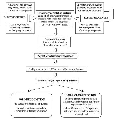
The overall flowchart of the PCM procedure is shown in Fig. 2.

Figure 2.

Detecting fold similarities with PCM: a flowchart of the overall procedure.

Results and Discussion

Remote Homologues.

Remote homologues in our test are defined as proteins with similar fold but sequence identity not more than 25%. In calculating sequence identity, only the structurally aligned positions, as indicated in the FSSP database (20), are considered. To judge whether two folds are similar to each other, we used both manual [SCOP (21)] and automated (FSSP) classifications of protein structures. SCOP, often referred to as the most reliable classification (30), involves expert judgment but provides no alignment information, whereas FSSP is objective but requires careful assessment to exclude proteins with the same local structural motif but different folds.

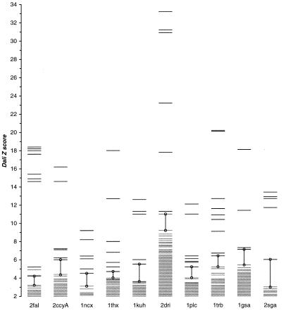
The extent of structural similarity in FSSP is provided by the DALI Z score (31). Although true remote homologues are found toward the top of the DALI list (ordered by the decreasing magnitude of Z score), the boundary between the true remote homologues and all other proteins is not well defined. We have observed that in most cases this boundary coincides with transition from “discrete” to “continuous” spectrum of Z scores and is marked with a prominent gap between adjacent Z scores in the DALI list (Fig. 3). Therefore, as an alternative to the classical, hard-cutoff model, Z_cutoff = β = const, we introduced a new, heuristic model, which can be formally described as:

3

The models were compared for their ability to find the true remote homologues (as indicated by SCOP) of 64 query proteins (Table 1) among those automatically detected in the FSSP database. The constants, β and ɛ, were optimized with criteria:

4

where ΔT (or ΔF) stands for the incremental number of true (or false) structural homologues with Z > Z_cutoff. With a higher cutoff we lose more true than false remote homologues (ΔT > ΔF), whereas with lower cutoff we include more false than true positives (ΔT < ΔF).

Figure 3.

Structural homologues in FSSP ordered by DALI Z score (31). For most queries the heuristic cutoff, i.e., the first large gap from the bottom, ΔZ = Z_i − Z_i+1 > ɛ (vertical lines), separates the true remote homologs (black lines on the top) from all other proteins (gray lines on the bottom) according to SCOP classification (21).

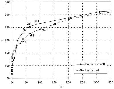
The optimal cutoffs, β = 6.5 and ɛ =0.5, find 58% and 67% of all true remote homologues, respectively, with less than 5% of false positives in both cases. Moreover, the heuristic cutoff, ɛ, works consistently better than the hard cutoff, β, for getting true remote homologues from the FSSP database (Fig. 4). Therefore, for proteins not yet classified by SCOP, we used the FSSP data with cutoff ɛ = 0.5 to establish their remote homology.

Figure 4.

Cutoff optimization on FSSP database. The number of true remote homologues (T) and other proteins (F) is determined for each value of the hard (gray lines) and heuristic (black lines) cutoffs. The optimal values (in bold) are chosen where ΔT/ΔF = 1.

Correlation of Physical Properties in Remote Homologues.

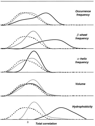
For a pair of remote homologues in FSSP we calculated the correlation coefficient of amino acid properties within a window of three, five, or seven residues (l = 1, 2, or 3, respectively) for each structurally aligned position by using Eq. 1. The sum of the coefficients, a total correlation, is compared with those obtained for the pairs of other members of the same fold with shuffled sequences as well as those for the pairs of other proteins with limited fold similarity according to FSSP. Among the five tested amino acid properties, hydrophobicity and β-sheet frequency are the two best properties to distinguish between true remote homologues of the globin fold and other proteins (Fig. 5). However, in general, hydrophobicity is the best property to detect remote homology by PCM for all fold types. The results described below were obtained by using this property.

Figure 5.

Distribution of the total correlation of physical properties in structural alignments of globin, 2FAL, and its true remote homologs (black lines) according to SCOP (21), proteins with limited structural similarity in FSSP (gray lines), and random sequences (dashed lines).

Fold Recognition by PCM.

Using each of 420 proteins representing the 64 well populated folds as query protein, we searched for its remote homologues among 1,390 proteins in the target set. With real or predicted secondary structure, the PCM method finds 178 or 167 true remote homologues, respectively. They correspond to more than 40% of all remote homologues within the 64 selected fold families.

The cutoff value for PCM predictions has been determined by the optimal ratio of true remote homologues and false positives (Eq. 4). The heuristic cutoff (Eq. 3) performs better than the hard one, and we found the optimal cutoff, ɛ = 0.9, is the same using PCM combined with either real or predicted secondary structure. The number of false positives with this cutoff is equal to 16% (8%) for PCM with predicted (real) secondary structure.

For several highly populated folds like globins, EF hand, periplasmic-binding proteins, and Rossman-fold, PCM detected more than 70% of their remote homologues. In most populated folds, α/β (TIM) barrels and immunoglobulins, which tolerate slight variations in size and topology, about 40% of remote homologues were recognized. For some queries, the true remote homologues were predicted with a Z score below the cutoff. For others, either the property correlation in structurally aligned regions is low, close to that in random sequences, or secondary structure pattern is not conserved between remote homologues.

Comparison with 1D-Threading Methods.

We compared the PCM method with four different 1D-threading methods available on the Internet: PredictProtein (11, 12), FoldFit (14), “Gon+predSS” (13), and H3P2 (15). Predictions were obtained for the same 64 queries by using the default parameters and fold library (Table 2) of each method. Because these methods use different fold libraries and scores, strict comparison is not possible. Therefore, success of fold recognition is determined by a uniform performance criteria: finding, at least one remote homologue in the top five proteins with the highest Z score. Before ranking, all predicted homologues with sequence identity more than 25% have been excluded. Because the identity of protein sequences is determined on the basis of structural alignment, pairs of proteins with low structural similarity (Z < 2.0 in FSSP) have been eliminated as well.

Table 2.

Fold recognition by different methods

Method	WWW address	Fold library		Number of correct predicted folds for query set
		Number of protein chains per domains	Maximum sequence identity
Predict protein	http://dodo.cpmc.columbia.edu/predictprotein	1,200	25%	44
Fold Fit	http://bonsai.lif.icnet.uk/foldfitnew	1,560	40%	38
H2P3	http://fold.doe-mbi.ucla.edu	2,943	Unknown	34
Gon + predSS		∼2,000	50%	48
PCM RealSS PredSS		1,390	25%	57
				47

The results of fold recognition are summarized in Table 2. The PCM method using real secondary structure tops the performance and provides the highest numbers of correct prediction of remote homologues: 57 of 64 query proteins found correct remote homologues, including 39 cases in which the true remote homologues appear as the first choices. With predicted secondary structure, the PCM method is comparable to “Gon+predSS,” the next best performer (Table 2). Comparing these three, we found that in two cases (1HTP and 1PUT) “Gon+predSS” is better than both versions of PCM and worse in the other four (1COLA, 1KUH, 1LIT, and 1WHTB). For some query proteins correct fold is recognized only by one method: 1GSA and 1PRTF by PCM, 1HTP and 1PUT by “Gon+predSS,” and 1ZYMA by PredictProtein. Combining the results of all of these methods (excluding PCM with real secondary structure), 57 of 64 queries found correct folds. Including additional properties of amino acids is likely to improve the PCM method further.

Comparison with psi-blast.

An advanced sequence-comparison method PSI-BLAST (18) was shown to be able to detect efficiently some remote homologues (32–36). We compared the PCM method with PSI-BLAST by using the same queries and target proteins for both methods, which allows us to compare the results directly (in contrast to comparison with 1D-threading, where each method uses its own fold library). All 420 remote homologues of the 64 most-populated folds were used as queries. PSI-BLAST predictions were obtained in three iterations. Two different e-value cutoffs, 10⁻³ and 10⁻⁴, that had been effective in other studies (32–36), were tested here. The other parameters were default.

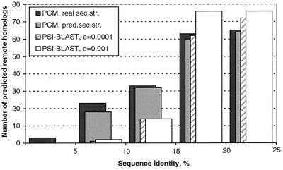
The PCM method with predicted secondary structure predicts more false positives (≈16%) than PSI-BLAST (≈2%). However, when compared for a similar number of predicted true remote homologues, PSI-BLAST is more successful in detecting remote homologues with sequence identities greater than 15%, whereas PCM does better for sequences with lower identities (Fig. 6). Therefore, a combination of these methods may be more efficient for predicting larger numbers of remote homologues.

Figure 6.

Distribution of remote homologues in the 64 query protein folds detected by PCM by using real or predicted secondary structure and psi-blast with different cutoffs.

Fold Recognition in Methanococcus jannaschii Genome.

We used PCM to discover remote homologues of the 64 protein folds from all the predicted proteins of the M. jannaschii genome (19). The predicted secondary structure was used for these proteins, and the real secondary structures were used for the query proteins. All 420 remote homologues of the 64 most-populated folds were used as queries to maximize the number of fold assignments. The cutoff, ɛ = 0.9, was applied to PCM predictions.

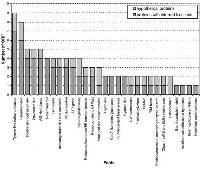
Of the 64 tested folds, 29 were detected in the genome of M. jannaschii (Fig. 7). Fold is assigned to 75 proteins; 22 of them listed in Table 3 currently are annotated as hypothetical proteins (Methanococcus jannaschii Genome Database: http://www.tigr.org/tdb/mdb/mjdb/mjdb.html).

Figure 7.

Protein folds detected by PCM in the M. jannaschii genome and their population.

Table 3.

PCM fold recognition of hypothetical proteins in genome of M. jannascii

ORF	Protein fold
MJ0018	Trypsin-like serine proteases
MJ0094	Cytochrome c
MJ0213	Viral coat and capsid proteins
MJ0425	Ferredoxin-like
MJ0590	5′–3′ exonuclease
MJ0644	Ferredoxin-like
MJ0870	TIM-barrel + Enolase and  muconate-lactonizing enzyme, N-term
MJ0917	Flavodoxin-like + ATP-grasp
MJ0954	PH-domain-like
MJ0996	Cysteine proteinases
MJ1147	Ferritin-like
MJ1178	Viral coat and capsid proteins
MJ1403	Double-stranded β-helix
MJ1428	4-helical cytokines
MJ1477	OB-fold
MJ1519	Class II aaRS and biotin synthetases
MJ1526	Trypsin-like serine proteases
MJ1535	Cysteine proteinases
MJ1542	Immunoglobulin-like β-sandwich
MJ1625	Cytochrome c
MJ1630	A/B-hydrolases
MJ1674	Reductase/isomerase/elongation factor  common domain + P-loop NTPase

Conclusions

We propose a new approach for detecting fold similarities between two proteins with weak or no sequence similarities by using the PCM of amino acid properties combined with predicted (or real) secondary structures of the proteins. The approach is based on our observation that physical properties of amino acid residues surrounding the corresponding residues in two proteins with the same fold are correlated along the sequences. Among the different properties tested in this work, hydrophobicity is shown to be the most strongly correlated property for all fold classes. In our future studies, we plan to incorporate the other properties that are correlated in some but not other fold classes.

The PCM method detects more than 40% of 420 remote homologues in the 64 selected folds. When the correct secondary structure is used, 89% of 64 query proteins, each representing a distinct fold, found at least one remote homologue among the top five choices. This number goes down to 73% after using predicted secondary structure. As the secondary structure prediction method improves, the performance of PCM is expected to improve as well. A test application of PCM method to the complete genome of M. jannaschii reveals its ability to infer fold information to hypothetical proteins as well as others with no fold information available with existing methods.

Compared with PSI-BLAST, our method demonstrates better sensitivity in detecting remote homologues with a sequence identity of less than 15%. Combined with existing methods, such as PSI-BLAST and/or 1D-threading, the PCM method can provide additional fold information for proteins with low sequence similarities.

Abbreviations

PCM

proximity correlation matrix

3D

three-dimensional

1D

one-dimensional

SCOP

structural classification of proteins

References

- 1.Smith T F, Waterman M S. J Mol Biol. 1981;147:195–197. doi: 10.1016/0022-2836(81)90087-5. [DOI] [PubMed] [Google Scholar]
- 2.Pearson W R, Lipman D J. Proc Natl Acad Sci USA. 1988;85:2444–2448. doi: 10.1073/pnas.85.8.2444. [DOI] [PMC free article] [PubMed] [Google Scholar]
- 3.Altschul S F, Gish W, Miller W, Myers E W, Lipman D J. J Mol Biol. 1990;215:403–410. doi: 10.1016/S0022-2836(05)80360-2. [DOI] [PubMed] [Google Scholar]
- 4.Bowie J U, Luthy R, Eisenberg D. Science. 1991;253:164–170. doi: 10.1126/science.1853201. [DOI] [PubMed] [Google Scholar]
- 5.Jones D T, Taylor W R, Thornton J M. Nature (London) 1992;358:86–89. doi: 10.1038/358086a0. [DOI] [PubMed] [Google Scholar]
- 6.Eisenhaber F, Persson B, Argos P. Crit Rev Biochem Mol Biol. 1995;30:1–94. doi: 10.3109/10409239509085139. [DOI] [PubMed] [Google Scholar]
- 7.Lemer C M, Rooman M J, Wodak S J. Proteins. 1995;23:337–355. doi: 10.1002/prot.340230308. [DOI] [PubMed] [Google Scholar]
- 8.Sternberg M J, Bates P A, Kelley L A, MacCallum R M. Curr Opin Struct Biol. 1999;9:368–373. doi: 10.1016/S0959-440X(99)80050-5. [DOI] [PubMed] [Google Scholar]
- 9.Sheridan R P, Dixon J S, Venkataraghavan R. Int J Peptide Protein Res. 1985;25:132–143. [Google Scholar]
- 10.Russell R B, Copley R R, Barton G J. J Mol Biol. 1996;259:349–365. doi: 10.1006/jmbi.1996.0325. [DOI] [PubMed] [Google Scholar]
- 11.Rost B. Proc Conf Intelligent Systems Mol Biol ISMB. 1995;95:314–321. [PubMed] [Google Scholar]
- 12.Rost B, Schneider R, Sander C. J Mol Biol. 1997;270:471–480. doi: 10.1006/jmbi.1997.1101. [DOI] [PubMed] [Google Scholar]
- 13.Fischer D, Eisenberg D. Protein Sci. 1996;5:947–955. doi: 10.1002/pro.5560050516. [DOI] [PMC free article] [PubMed] [Google Scholar]
- 14.Russell R B, Saqi M A S, Sayle R A, Bates P A, Sternberg M J E. Protein Eng. 1998;11:1–9. doi: 10.1093/protein/11.1.1. [DOI] [PubMed] [Google Scholar]
- 15.Rice D, Eisenberg D. J Mol Biol. 1997;267:1026–1038. doi: 10.1006/jmbi.1997.0924. [DOI] [PubMed] [Google Scholar]
- 16.Russell R B, Saqi M A S, Sayle R A, Bates P A, Sternberg M J E. J Mol Biol. 1997;269:423–439. doi: 10.1006/jmbi.1997.1019. [DOI] [PubMed] [Google Scholar]
- 17.Gerstein M. Fold Des. 1998;3:497–512. doi: 10.1016/S1359-0278(98)00066-2. [DOI] [PubMed] [Google Scholar]
- 18.Altschul S F, Madden T L, Schaffer A A, Zhang J, Zhang Z, Miller W, Lipman D J. Nucleic Acids Res. 1997;25:3389–3402. doi: 10.1093/nar/25.17.3389. [DOI] [PMC free article] [PubMed] [Google Scholar]
- 19.Bult C J, White O, Olsen G J, Zhou L, Fleischmann R D, Sutton G G, Blake J A, FitzGerald L M, Clayton R A, Gocayne J D, et al. Science. 1996;273:1058–1073. doi: 10.1126/science.273.5278.1058. [DOI] [PubMed] [Google Scholar]
- 20.Holm L, Sander C. Nucleic Acids Res. 1998;26:316–319. doi: 10.1093/nar/26.1.316. [DOI] [PMC free article] [PubMed] [Google Scholar]
- 21.Murzin A G, Brenner S E, Hubbard T J P, Chothia C. J Mol Biol. 1995;247:536–540. doi: 10.1006/jmbi.1995.0159. [DOI] [PubMed] [Google Scholar]
- 22.Tomii K, Kanehisa M. Protein Eng. 1996;9:27–36. doi: 10.1093/protein/9.1.27. [DOI] [PubMed] [Google Scholar]
- 23.Fauchere J L, Pliska V. J Eur J Med Chem. 1983;18:369–375. [Google Scholar]
- 24.Zamyatin A A. Prog Biophys Mol Biol. 1972;24:107–123. doi: 10.1016/0079-6107(72)90005-3. [DOI] [PubMed] [Google Scholar]
- 25.Chou P Y, Fasman G D. Adv Enzymol. 1978;47:45–148. doi: 10.1002/9780470122921.ch2. [DOI] [PubMed] [Google Scholar]
- 26.Jones D T, Taylor W R, Thornton J M. CABIOS. 1992;8:275–282. doi: 10.1093/bioinformatics/8.3.275. [DOI] [PubMed] [Google Scholar]
- 27.Kabsh W, Sander C. Biopolymers. 1983;22:2577–2637. doi: 10.1002/bip.360221211. [DOI] [PubMed] [Google Scholar]
- 28.Jones D T. J Mol Biol. 1999;292:195–202. doi: 10.1006/jmbi.1999.3091. [DOI] [PubMed] [Google Scholar]
- 29.Needleman S B, Wunsch C D. J Mol Biol. 1970;48:443–453. doi: 10.1016/0022-2836(70)90057-4. [DOI] [PubMed] [Google Scholar]
- 30.Gerstein M, Levitt M. Protein Sci. 1998;7:445–456. doi: 10.1002/pro.5560070226. [DOI] [PMC free article] [PubMed] [Google Scholar]
- 31.Holm L, Sander C. Nucleic Acids Res. 1994;22:3600–3609. [PMC free article] [PubMed] [Google Scholar]
- 32.Teichmann S A, Park J, Chothia C. Proc Natl Acad Sci USA. 1998;95:14658–14663. doi: 10.1073/pnas.95.25.14658. [DOI] [PMC free article] [PubMed] [Google Scholar]
- 33.Huynen M, Doerks T, Eisenhaber F, Orengo C, Sunyaev S, Yuan Y P, Bork P. J Mol Biol. 1998;280:323–326. doi: 10.1006/jmbi.1998.1884. [DOI] [PubMed] [Google Scholar]
- 34.Salamov A A, Suwa M, Orengo C A, Swindells M B. Protein Sci. 1999;8:771–777. doi: 10.1110/ps.8.4.771. [DOI] [PMC free article] [PubMed] [Google Scholar]
- 35.Wolf Y I, Brenner S E, Bash P A, Koonin E V. Genome Res. 1999;9:17–6. [PubMed] [Google Scholar]
- 36.Park J, Karplus K, Barrett C, Hughey R, Haussler D, Hubbard T, Chothia C. J Mol Biol. 1998;284:1201–1210. doi: 10.1006/jmbi.1998.2221. [DOI] [PubMed] [Google Scholar]