A Test for Genetic Association that Incorporates Information about Deviation from Hardy-Weinberg Proportions in Cases

Abstract

For assessment of genetic association between single-nucleotide polymorphisms (SNPs) and disease status, the logistic-regression model or generalized linear model is typically employed. However, testing for deviation from Hardy-Weinberg proportion in a patient group could be another approach for genetic-association studies. The Hardy-Weinberg proportion is one of the most important principles in population genetics. Deviation from Hardy-Weinberg proportion among cases (patients) could provide additional evidence for the association between SNPs and diseases. To develop a more powerful statistical test for genetic-association studies, we combined evidence about deviation from Hardy-Weinberg proportion in case subjects and standard regression approaches that use case and control subjects. In this paper, we propose two approaches for combining such information: the mean-based tail-strength measure and the median-based tail-strength measure. These measures integrate logistic regression and Hardy-Weinberg-proportion tests for the study of the association between a binary disease outcome and an SNP on the basis of case- and control-subject data. For both mean-based and median-based tail-strength measures, we derived exact formulas to compute p values. We also developed an approach for obtaining empirical p values with the use of a resampling procedure. Results from simulation studies and real-disease studies demonstrate that the proposed approach is more powerful than the traditional logistic-regression model. The type I error probabilities of our approach were also well controlled.

Introduction

Traditionally, regression approaches have been used for the assessment of the genetic association between single-nucleotide polymorphisms (SNPs) and disease status and have been applied to detect a variety of disease-causing SNPs.^1–8 However, the regression approaches do not integrate information that is available from other sources, such as deviation from Hardy-Weinberg (hereafter, HW) proportion in cases. Therefore, we propose an approach for gene-association assessment that integrates the HW-proportion information in the regression approaches.

The HW proportion is one of the most important principles in population genetics. Consider a simple case with two alleles, A and a, at a single locus. If the allele frequency of A is denoted as p, then the frequency of a is (1 − p). Under the assumption of HW proportion in the population, the frequencies of three possible genotypes, (A, A), (A, a), and (a, a), are the products of allele frequencies p², 2p(1 − p), and (1 − p)², respectively.

In case-control association studies, the HW proportion assessed in control subjects is widely used as a quality-control tool for identifying genotyping errors.^9–12 However, researchers also suggest that deviation from HW proportion—which can be evaluated via a comparison of the difference between observed genotype frequencies and the corresponding expected frequencies ¹³—among cases (patients) can provide additional evidence for a real association between SNP genotypes and disease outcomes.^14–18 Thus, testing for deviation from HW proportion could be another approach for the study of genetic association.

To develop a more powerful statistical test for genetic association, we combined evidence from HW-proportion deviation and from regression approaches to perform the case-control association study. A mean-based tail-strength (TS) measure for association study is proposed, in which we have combined two different hypothesis tests, (1) the logistic-regression model and (2) the test for deviation from HW proportion in case subjects. Although these two hypothesis tests are quite different, given that they use different test statistics and test different aspects of the dataset, both tests can provide information about the association between SNPs and diseases. These two tests are also statistically correlated. Both cases and controls are used in logistic regression, whereas the HW-proportion test, as proposed, uses data from cases only. The proposed mean-based TS measure allows dependence between these two tests. We further extended the mean-based TS measure to a median-based TS (TSM) measure by using median values instead of expected values. For both measures, we derived the exact formulas for calculation of p values. We also propose an approach for estimating empirical p values with the use of a resampling procedure.

On the basis of the exact and empirical results from simulated data and real biological examples, our proposed approach is more powerful than the traditional association study approaches, achieving higher power than that achieved by each individual test and maintaining good control over type I error probabilities. This combined approach is also valid for performing association studies with the use of other statistical methods, including piecewise logistic regression, nonparametric logistic regression, and functional logistic regression.

Material and Methods

For simplicity, we assume two alleles, A and a, at a locus, with A as the deleterious allele and a as the normal allele. We use a categorical random variable, X = {0, 1, 2}, to denote the three genotypes, (A, A), (A, a), and (a, a). Note that the values of the random variable correspond to the number of copies of the A allele. This coding assumes an additive model, but different coding for representing a dominant or recessive model can also be used. Our proposed approach is not restricted to an additive model. We defined another categorical random variable, Y = {0,1}, to indicate the case-control status, with 0 representing individuals in the control group and 1 representing individuals in the case group.

Given a dataset of observations of random variables X and Y corresponding to the genotypes of a SNP and the case-control outcomes, respectively, two hypothesis tests can be applied for detection of the association between disease and SNP: the logistic-regression approach, using cases and controls, and the test for deviation from HW proportion among cases. Our goal was to combine these two tests to achieve a more powerful statistical test for association study.

Tail-Strength Measures

A tail-strength (TS) measure was recently developed by Taylor and Tibshirani¹⁹ for the study of large amounts of microarray data. This measure assesses the overall univariate strength of a large set of features in microarray and other genomic studies. We applied and extended the TS measure to the problem of integrating the logistic-regression association approach and the test for deviation from HW proportion, as briefly described below.

Consider m p values p_i, i = 1,…m, with respect to the m null hypotheses. The global hypothesis is that all the individual hypotheses hold simultaneously. Now denote p₍₁₎ ≤ p₍₂₎ ≤ …p_(m) as the ordered p values. Thus, the TS measure is defined as follows:

$$TS(p_1,p_2,\dots p_m)=\frac{1}{m}\sum _{i=1}^m\left(1-p_{\left(i\right)}\frac{m+1}{i}\right).$$ (1)

Note that under the null hypothesis, each p_i has uniform distribution, so that the ordered p value p_(i) follows a beta distribution with the mean as i/(m + 1). Hence, the test statistic TS has an expectation of zero under the null hypothesis. Taylor and Tibshirani showed in their paper that the TS measure is closely related to the false-discovery rate (FDR) approach to multiple-hypothesis testing. From this property, they derived the asymptotic distribution for TS when m is large, which is normally distributed with a mean of 0 and a variance of 1/m. They also showed that the TS measure has a close relationship to a weighted area under a receiver operating characteristic (ROC) curve.

The TS measure calculates the linear combination of the difference between each p value and its expected value. In this form, as Equation (1), it gives more weight to the smaller p values so that it is more sensitive to deviations in the tail. When the TS value approaches 1, it shows that there are more small p values than we would expect by chance and then indicates the evidence against the global-null hypothesis.¹⁹ In this way, we would expect that the test statistic TS for the global hypothesis should be more powerful than each individual test.

In our specific problem, the asymptotic distribution of TS cannot be applied. Recall that we now consider two hypothesis tests, which are correlated. We are proposing to use the TS measure for combining the logistic-regression association model that uses cases and controls for testing H₀₁ (H₀₁: Association does not exist between SNP and disease) with evidence derived from the Hardy-Weinberg proportion test for testing H₀₂ (H₀₂: HW proportion exists among case subjects).

Consider a single SNP, X. Recall that Y is the random variable corresponding to the outcomes of the disease of concern. Let T₁ be the test statistic for using the logistic regression model to detect the association between X and Y (i.e., H₀₁) and T₂ be the test statistic for testing deviation from the HW proportion among cases (i.e., H₀₂). In our proposal, we used the likelihood-ratio test for logistic regression and performed the exact test for testing HW-proportion deviation in the case group.^13,20,21 Let p₁ and p₂ be the p values that correspond to T₁ and T₂. Accordingly, p₍₁₎ and p₍₂₎ are the ordered p values. Therefore, we can define the tail-strength measure that combines the two p values as follows:

$$TS(p_1,p_2)=\frac{1}{2}\left(\left(1-p_{\left(1\right)}\times 3\right)+\left(1-p_{\left(2\right)}\times \frac{3}{2}\right)\right)$$ (2)

to test the global-null hypothesis that the SNP is not associated with disease.

The domain of random variable TS is [−1.25, 1], given that 0 ≤ p₍₁₎ ≤ p₍₂₎ ≤ 1. Recall that p₍₁₎ and p₍₂₎ follow a beta distribution under the null hypothesis. Using a bivariate transformation, we can derive the explicit formula for the probability-density function of the tail-strength random variable TS:

$$f_{TS}\left(x\right)=\{\begin{array}{cc}\frac{8}{27}\left(\frac{5}{2}+2x\right),& ifx\in [-1.25,0.25],\\ \frac{32}{27}\left(1-x\right),& ifx\in (0.25,1].\end{array}$$ (3)

Given an observation of TS^∗, the exact p values of random variable TS can be calculated by a simple integral of the above equation such that

$$p\mathit{value}=P(TS>T{S}^{\ast })={\int }_{T{S}^{\ast }}^1{f}_{TS}\left(x\right)dx$$ (4)

TS is a measure that uses means for comparison with observed p values. But in some situations, median-based estimators are more robust for extreme observations. Because we are dealing with small p values, a median-based tail-strength measure might be more appropriate under some circumstances, whereas a mean-based measure might apply to other situations. Therefore, we developed a measure for the assessment of tail strength with the use of median values. We call it the tail-strength median (TSM) measure, in which the linear combination of the difference between p values and corresponding median values, rather than expected values, is calculated under the null hypothesis. The median values for p₍₁₎ and p₍₂₎ are $1-1/\sqrt{2}$ and $1/\sqrt{2}$, respectively. Therefore, the TSM measure can be defined as

$$TSM(p_1,p_2)=\frac{1}{2}\left(\left(1-p_{\left(1\right)}\times \frac{\sqrt{2}}{\sqrt{2}-1}\right)+\left(1-p_{\left(2\right)}\times \sqrt{2}\right)\right)$$ (5)

for testing the global-null hypothesis for the association between the SNP and the disease in question.

We derived the explicit form for the probability-density function of the tail-strength-median random variable TSM. In this situation, the domain of the random variable is $[-\sqrt{2},1]$.

$$g_{TSM}\left(x\right)=\{\begin{array}{cc}\frac{2\sqrt{2}(\sqrt{2}-1)}{\sqrt{2}+1}\left(\sqrt{2}+x\right),& ifx\in [-\sqrt{2},1-\frac{1}{\sqrt{2}}],\\ \frac{2\sqrt{2}}{\sqrt{2}+1}\left(1-x\right),& ifx\in (1-\frac{1}{\sqrt{2}},1]\end{array}.$$ (6)

Given an observation of TSM^∗, the exact p values of random variable TSM can be calculated by a simple integral of the above equation, such that

$$p\mathit{value}=P(TSM>TS{M}^{\ast })={\int }_{TS{M}^{\ast }}^1{g}_{TSM}\left(x\right)dx$$ (7)

Compared with TS, TSM assigns even more weight to the smaller p values but less weight to the bigger p values. Note that the FDR approach can be explained as a procedure in which ordered p values are compared with the functions of their expected values.²² Using similar thinking, we now consider median values of ordered p values instead of expected p values. Consequently, the TSM measure also has a close relationship to the FDR approach to multiple-hypothesis testing. (The derivations for the explicit forms of density functions of TS and TSM and associated p values are given in Appendix 1.)

Permutation Tests

Although the exact p values of TS and TSM are simple and straightforward to compute and interpret, the derivations of underlying assumptions might make the exact p values based on the explicit formulas either too conservative or too liberal. Therefore, we also proposed an approach for estimating empirical p values of TS and TSM with the use of a permutation procedure. For each permutation step, we resample the SNP-values vector by using the genotype frequencies calculated from the allele frequencies of the whole dataset, including the SNP values in both case and control groups, but keep all the other random-variable vectors (e.g., covariates) unchanged. By resampling the SNP values, we ensure that there will be no association between the outcomes and the SNP. The empirical p values for both tests are estimated by the proportion of TS or TSM values resulting from permutations that are greater than the observed TS or TSM values. The performance of the permutation tests is evaluated in Appendix 2.

Simulation Studies

We examined the performance of the proposed approach by performing simulation studies first and then applying the approach to real diseases. In order to simulate data related to the genotypes of SNPs and the outcomes of case-control status, two logistic models were used. In the first simulated model, we considered only SNPs as the risk factors associated with diseases and specified the frequencies of genotypes and the odds ratios (ORs) of the logistic model. We performed further simulation studies based on a real disease (lung cancer) model, involving SNPs and other statistically significant risk factors. The second simulated model was based on a lung-cancer study of current smokers.²³ We studied different predefined genotype frequencies and ORs of SNPs while citing those of all the other risk factors from the literature. In the following sections, we describe the models for these simulation studies and report the results accordingly.

Model 1

Considering two independent SNPs at two different genetic loci, X₁ and X₂, we defined the corresponding logistic model of the association between SNPs and case-control outcomes as

$$\text{Logit}\left(P(Y=1)\right)={\mathrm{\beta }}_0+{\mathrm{\beta }}_1{X}_1+{\mathrm{\beta }}_2{X}_2$$

First, we simulated genotypes of X₁ and X₂ under the null hypothesis—that is, under the assumption of HW proportion in the general population. In this model, unless otherwise specified, we assumed minor-allele frequencies of 10% for SNP X₁ and 40% for SNP X₂. Given the dataset of realizations of SNPs X₁ and X₂, one could randomly generate disease status for each individual according to the logistic model above. In this way, we simulated a large amount of data on the population of interest, then randomly sampled 500 disease-related cases along with 500 normal controls from the population, with the assumption of an alternative global hypothesis. Note that we assumed HW proportion in the general population; however, after simulation, cases might not be in HW proportion. Thus, given the data set simulated from the above model, we could evaluate the performance of the TS measure and the TSM measure proposed to combine the two hypothesis tests.

We generated six datasets from Model 1, with different ORs associated with SNP X₁, while either observing or not observing the second SNP, X₂. The specific parameters for different datasets are given in Table 1. β₀ remained fixed in all the datasets. Two ORs for SNP X₁, OR = 1.35 and OR = 1.65, were studied. According to Table 1, SNP X₂ could be insignificantly associated with disease (OR = 1) and observed (genotyped), insignificantly associated with disease and unobserved, significantly associated with disease (OR = 1.35) and observed, or significantly associated with disease (OR = 1.35) but unobserved. For example, Data set 3 was generated at β₀ = −2, β₁ = 0.3, and β₂ = 0.3, and SNP X₂ was observed. Averages of significance reported in the Results section are based on 100 replicates, which included 500 cases and 500 controls. The significance of each replicate was determined by both exact p values and empirical p values derived from the permutation tests described above.

Table 1.

Simulation Parameters for Data Sets Generated from Model 1

Data Set	${\beta }_0$	${\beta }_1$	${\beta }_2$	SNP 2
Data 1	−2.0	0.3 (OR = 1.35)	1.0 × 10−10 (OR = 1)	Observed
Data 2	−2.0	0.3 (OR = 1.35)	1.0 × 10−10 (OR = 1)	Unobserved
Data 3	−2.0	0.3 (OR = 1.35)	0.3 (OR = 1.35)	Observed
Data 4	−2.0	0.3 (OR = 1.35)	0.3 (OR = 1.35)	Unobserved
Data 5	−2.0	0.5 (OR = 1.65)	0.3 (OR = 1.35)	Observed
Data 6	−2.0	0.5 (OR = 1.65)	0.3 (OR = 1.35)	Unobserved

Model 2

We simulated data from a lung-cancer model based on the study of Spitz et al.,²³ as shown in Table 2. All the statistically significant risk factors associated with lung cancer among current smokers are listed, including a history of emphysema, exposure to dust, exposure to asbestos, family history of any cancer, a history of hay fever, and smoking intensity (pack-years), with the cut points based on the quartile of current smoker pack-years in control subjects. For the purpose of our study, two more factors were considered: smoking status and existence of a single SNP. We defined two models with respect to smoking status. The two lung-cancer models correspond to two groups of people: the general lung-cancer population and the current-smoker lung-cancer population. We, therefore, refer to them as the “general model” and the “current-smoker model.” When we only considered the current-smoker lung-cancer population, we removed the smoking risk factor from the logistic model; when we studied the whole population, smoking status was included and was an extremely significant variable in the model.²⁴

Table 2.

Lung-Cancer Models

Risk Factors	Coefficients of Logistic Model	Prevalence
Intercept	−0.7173
SNP	0.3 (OR = 1.35)/0.5 (OR = 1.65)
Smoking	2.3 (OR = 9.97)/0.0 (OR = 1)	21.0%
Emphysema	0.7561 (OR = 2.13)	35.0%
Dust exposure	0.3067 (OR = 1.36)	21.0%
Asbestos exposure	0.4109 (OR = 1.51)	23.7%
Family history	0.3859 (OR = 1.47)	7.1%
Hay fever	0.4047 (OR = 1.50)	9.0%
Pack-years
28-41.9	0.2219 (OR = 1.25)	25.0%
42-57.4	0.3747 (OR = 1.45)	25.0%
≥57.5	0.6151 (OR = 1.85)	25.0%

For the purpose of simulation, all the ORs of the risk factors, except SNP, were from the Spitz et al. study.²³ The prevalences of the risk factors cited came from different papers or statistical summaries: smoking,²³ history of emphysema,²⁵ exposure to dust,²⁶ exposure to asbestos,²⁷ family history of any cancer,²⁸ and history of hay fever.²⁵ Table 2 lists the parameters that we used to simulate the data according to the model described above. For example, the OR for a history of emphysema was 2.13, and its prevalence was set to 35%. The OR for smoking status was defined as 1 in the current-smoker model and as approximately 10 in the general model, because smoking is the most significant risk factor for lung cancer.

In the lung-cancer models, we wanted to demonstrate the performance of our approach for SNP association with different logistic coefficients (ORs) and different genotype frequencies. Therefore, for each model, we generated six datasets with respect to different ORs of the SNP, as well as different genotype frequencies, on the basis of the ORs and prevalences listed in Table 2 for all the other risk factors for lung cancer. We exclusively studied two ORs for the SNP, OR = 1.35 and OR = 1.65, as in Model 1. For each OR, we used minor-allele frequencies of 10%, 30%, and 50% (from rare to more common). We used the same approach for simulation and the assumption of the alternative hypothesis used in Model 1, and 100 replicates were generated for each scenario, including 500 cases and 500 controls in each replicate. The significance of each replicate was also determined by both exact p values and empirical p values.

Type I Error Estimate

We performed additional simulations to examine the type I error probability of our approach under the global-null hypothesis of no association between the SNP and the disease. For both simulation Model 1 and Model 2, we used the same settings as above, except that the coefficient of SNP for the logistic model was set to zero (OR = 1). We generated four datasets from Model 1, which correspond to data sets 1–4 in Table 1, except that β₁ = 0 (data sets 5 and 6 are exactly the same as Data sets 3 and 4 under the null hypothesis). To test Model 2, we generated three datasets from the general model with respect to different genotype frequencies, along with three datasets from the current-smoker model. For each configuration, 10,000 simulated replicates were generated, each with 500 cases and 500 controls.

Results

Model 1

All of the resulting logistic-regression p values, HW-proportion test p values, empirical p values of TS and TSM, and exact p values of TS and TSM are reported in Table 3. For all tests, we reported the average results, grouped with respect to TS and TSM. For instance, for data set 3 (generated with β₀ = −2.0, β₁ = 0.3, and β₂ = 0.3, and in which SNP X₂ was observed; see Table 1), on the basis of 100 replicates, the average p value obtained from logistic regression with the use of cases and controls was 0.013, whereas the average p value from the HW-proportion test in the case group was 0.0288. After applying the TS measure and the TSM measure, the average empirical p values from 100,000 permutations were 0.0008 and 0.0009 for TS and TSM, respectively, and the average exact p values calculated from Equations (4) and (7) were 0.0012 and 0.0013 for TS and TSM, respectively.

Table 3.

Average p Values from Different Tests in Simulations for Model 1

Data Set	p-logita	p-HWPb	TS		TSM
			Empirical TS p Values	Exact TS p Values	Empirical TSM p Values	Exact TSM p Values
Data 1	0.0099	0.0264	0.0006	0.0009	0.0006	0.0009
Data 2	0.0135	0.0257	0.0007	0.0010	0.0008	0.0011
Data 3	0.0130	0.0288	0.0008	0.0012	0.0009	0.0013
Data 4	0.0147	0.0254	0.0009	0.0012	0.0009	0.0013
Data 5	0.0044	0.0261	0.0004	0.0006	0.0004	0.0006
Data 6	0.0041	0.0246	0.0004	0.0005	0.0004	0.0006

^ap value from logistic-regression test.

^bp value from HW-proportion test.

We obtained more significant p values by using both TS and TSM measures as compared with those obtained with the use of logistic regression. When the SNP X₂ was significantly associated with the disease, whether or not we could observe the values of SNP X₂, we obtained nearly identical exact and empirical p values for both measures (see results for data sets 3–6 from Table 3). The empirical and exact p values were very similar, but the empirical approach yielded slightly more liberal p values, possibly because we used 100,000 permutations. However, the exact p values were still satisfactory in this situation, because they are computationally more practical than the use of permutation tests.

Because all the replicates in each dataset were simulated under the alternative hypothesis, we examined the statistical power of our approach. Table 4 shows the observed power based on 100 replicates for the six data sets (for which average p values are reported in Table 3) at the nominal significance levels 0.01, 0.005, and 0.001. The power for logistic regression, as well as the empirical power and exact power for both TS and TSM, are reported in Table 4. The results are grouped into two panels with respect to the two tail-strength measures. Given that bigger ORs imply a more-significant association between factors and diseases, we would expect to see more small p values in this situation. So, it is not surprising that the power is higher when the OR increases from 1.35 to 1.65 in the logistic-regression model. After we integrated evidence from the HW-proportion test among case subjects, our approach for association study gained considerable power compared to that of the logistic-regression model. For instance, the observed powers for data set 3 with the use of logistic regression were 63%, 43%, and 22% for the defined significance levels 0.01, 0.005, and 0.001, respectively. When the TS measure was used, the observed empirical powers were 100%, 100%, and 76% at significance levels 0.01, 0.005, and 0.001, respectively; and the observed exact powers were 100%, 96%, and 56%, respectively. Overall, the performance of the TSM measure was similar to that of the TS measure in this model.

Table 4.

Power Comparison at 0.01, 0.005, and 0.001 Significance Levels in Simulations for Model 1

Data Set	Power for Logistic Model			Power for TS						Power for TSM
				Empirical Powers			Exact Powers			Empirical powers			Exact powers
	0.01	0.005	0.001	0.01	0.005	0.001	0.01	0.005	0.001	0.01	0.005	0.001	0.01	0.005	0.001
Data 1	0.67	0.54	0.26	1.00	1.00	0.80	1.00	1.00	0.73	1.00	1.00	0.81	1.00	0.99	0.73
Data 2	0.51	0.32	0.16	1.00	1.00	0.80	1.00	0.98	0.63	1.00	0.99	0.74	1.00	0.98	0.63
Data 3	0.63	0.43	0.22	1.00	1.00	0.76	1.00	0.96	0.56	1.00	0.99	0.76	1.00	0.95	0.57
Data 4	0.49	0.40	0.21	1.00	1.00	0.67	1.00	0.99	0.58	1.00	1.00	0.66	1.00	0.97	0.57
Data 5	0.86	0.85	0.66	1.00	1.00	0.90	1.00	1.00	0.87	1.00	1.00	0.89	1.00	0.99	0.87
Data 6	0.87	0.83	0.63	1.00	1.00	0.93	1.00	0.99	0.92	1.00	0.99	0.93	1.00	0.99	0.92

Model 2

Tables 5–8 report all the resulting average p values and powers for the logistic-regression approach, HW-proportion test among the case group, and empirical and exact tests for both TS and TSM for both lung-cancer-simulation models.

Table 5.

Average p Values from Different Tests in Simulations for the General Model

Data Sets	p-logita	p-HWPb	TS		TSM
			Empirical TS p Values	Exact TS p Values	Empirical TSM p Values	Exact TSM p Values
β = 0.3 (OR = 1.35)
(0.81, 0.18, 0.01)	0.0135	0.0287	0.0008	0.0012	0.0009	0.0013
(0.49, 0.42, 0.09)	0.0079	0.0247	0.0006	0.0007	0.0006	0.0007
(0.25, 0.50, 0.25)	0.0057	0.0272	0.0006	0.0007	0.0006	0.0006
β = 0.5 (OR = 1.65)
(0.81, 0.18, 0.01)	0.0069	0.0278	0.0005	0.0007	0.0005	0.0007
(0.49, 0.42, 0.09)	0.0005	0.0251	0.0003	0.0003	0.0002	0.0003
(0.25, 0.50, 0.25)	0.0002	0.0241	0.0003	0.0003	0.0002	0.0002

^ap value from logistic-regression test.

^bp value from HW-proportion test.

Table 6.

Power Comparison at 0.01, 0.005, and 0.001 Significance Levels in Simulations for the General Model

Data Sets	Power for Logistic Model			Power for TS						Power for TSM
				Empirical Powers			Exact Powers			Empirical Powers			Exact Powers
	0.01	0.005	0.001	0.01	0.005	0.001	0.01	0.005	0.001	0.01	0.005	0.001	0.01	0.005	0.001
β = 0.3 (OR = 1.35)
(0.81, 0.18, 0.01)	0.47	0.41	0.17	1.00	1.00	0.74	1.00	0.97	0.60	1.00	0.99	0.72	1.00	0.97	0.58
(0.49, 0.42, 0.09)	0.72	0.61	0.39	1.00	1.00	0.85	1.00	0.98	0.81	1.00	0.98	0.84	1.00	0.98	0.80
(0.25, 0.50, 0.25)	0.83	0.75	0.50	1.00	1.00	0.83	1.00	0.99	0.83	1.00	0.99	0.83	1.00	0.99	0.83
β = 0.5 (OR = 1.65)
(0.81, 0.18, 0.01)	0.76	0.67	0.47	1.00	1.00	0.87	1.00	1.00	0.76	1.00	1.00	0.87	1.00	0.99	0.76
(0.49, 0.42, 0.09)	0.98	0.98	0.94	1.00	1.00	0.99	1.00	1.00	0.99	1.00	1.00	0.99	1.00	1.00	0.99
(0.25, 0.50, 0.25)	1.00	1.00	0.96	1.00	1.00	1.00	1.00	1.00	1.00	1.00	1.00	1.00	1.00	1.00	1.00

Table 7.

Average p Values from Different Tests in Simulations for Current-Smoker Model

Data Sets	p-logita	p-HWPb	TS		TSM
			Empirical TS p Values	Exact TS p Values	Empirical TSM p Values	Exact TSM p Values
β = 0.3 (OR = 1.35)
(0.81, 0.18, 0.01)	0.0124	0.0274	0.0007	0.0011	0.0008	0.0011
(0.49, 0.42, 0.09)	0.0049	0.0228	0.0004	0.0005	0.0004	0.0005
(0.25, 0.50, 0.25)	0.0058	0.0242	0.0005	0.0005	0.0005	0.0005
β = 0.5 (OR = 1.65)
(0.81, 0.18, 0.01)	0.0049	0.0255	0.0003	0.0005	0.0003	0.0005
(0.49, 0.42, 0.09)	0.0007	0.0251	0.0003	0.0003	0.0003	0.0003
(0.25, 0.50, 0.25)	0.0001	0.0263	0.0003	0.0003	0.0002	0.0003

^ap value from logistic-regression test.

^bp value from HW-proportion test.

Table 8.

Power Comparison at 0.01, 0.005, and 0.001 Significance Levels in Simulations for Current-Smoker Model

Data Sets	Power for Logistic Model			Power for TS						Power for TSM
				Empirical Powers			Exact Powers			Empirical Powers			Exact Powers
	0.01	0.005	0.001	0.01	0.005	0.001	0.01	0.005	0.001	0.01	0.005	0.001	0.01	0.005	0.001
β = 0.3 (OR = 1.35)
(0.81, 0.18, 0.01)	0.57	0.46	0.20	1.00	1.00	0.78	1.00	0.99	0.61	1.00	1.00	0.76	1.00	0.96	0.61
(0.49, 0.42, 0.09)	0.89	0.69	0.49	1.00	0.99	0.93	1.00	0.99	0.90	1.00	0.99	0.92	1.00	0.99	0.91
(0.25, 0.50, 0.25)	0.80	0.74	0.51	1.00	1.00	0.91	1.00	1.00	0.88	1.00	1.00	0.91	1.00	1.00	0.90
β = 0.5 (OR = 1.65)
(0.81, 0.18, 0.01)	0.83	0.79	0.55	1.00	1.00	0.87	1.00	0.99	0.76	1.00	1.00	0.96	1.00	0.99	0.89
(0.49, 0.42, 0.09)	0.98	0.98	0.92	1.00	1.00	0.99	1.00	1.00	0.99	1.00	1.00	0.99	1.00	1.00	0.99
(0.25, 0.50, 0.25)	1.00	0.99	0.99	1.00	1.00	0.99	1.00	1.00	0.99	1.00	1.00	0.99	1.00	1.00	0.99

Consider the general model first. In this model, the OR of smoking status is about 10. The average p values are shown in Table 5. The results are arranged into two panels with respect to TS and TSM. As expected, we see trends of decreasing average p values for logistic regression as the OR increases from 1.35 to 1.65 and as the minor allele frequency increases from 10% to 50%. For example, a dataset was generated under the scenario of OR = 1.65 and genotype frequencies of 81%, 18%, and 1%. On the basis of 100 replicates, and under the alternative hypothesis of an association existing between the SNP and lung cancer, the average p value obtained from logistic regression analysis was 0.0069, and the average p value for the HW-proportion test among case subjects was 0.0278. For both TS and TSM, the average empirical p value for this scenario, based on 100,000 permutations, was 0.0005, and the average exact p value calculated from the exact formula was 0.0007. Even when the logistic p values were already highly significant, our approach still provided similarly significant empirical and exact p values. For example, the logistic p value of the data set generated with OR = 1.65 and allele frequencies 25%, 50%, and 25% was 0.0002, and the empirical and exact p values were 0.0003 and 0.0002 for both measures, respectively. The results demonstrate that our approach achieves more-significant p values by integrating the evidence from the HW-proportion test in the case group and that from association from traditional logistic regression with cases and controls used.

Table 6 gives the corresponding power-comparison results at the nominal significance levels 0.01, 0.005, and 0.001. Two panels with respect to TS and TSM are shown in the table. Our approach resulted in much-higher power than did the logistic-regression approach. All the empirical powers and exact powers were close to 100% at significance levels 0.01 and 0.005 and were much higher at level 0.001 as compared to those from logistic regression. Even for the data set generated with OR = 1.65 and genotype frequencies 25%, 50%, and 25%, which might be considered to already have enough power with the use of logistic regression, we still saw an increase in the power from 96% to 100% at significance level 0.001. In addition to the results shown in Tables 5 and 6, we also studied the scenarios using OR = 2.01 (coefficient of logistic model = 0.7). Similar results were obtained. For example, when the genotype frequencies 81%, 18%, and 1% and OR = 2.01 were assumed, the observed powers for logistic regression were 93%, 91%, and 77% for significance levels 0.01, 0.005, and 0.001, respectively. For both the proposed measures, the empirical powers and exact powers were approximately 100% at levels 0.01 and 0.005 and about 95% at level 0.001, based on 100 replicates. Like the results for Model 1, the TSM measure had results similar to those of the TS measure, which is also shown in Tables 5 and 6.

The average p values and power-comparison results for the current-smoker model are reported in Tables 7 and 8. It is not surprising that more significant average p values for logistic regression are seen compared to those in the general model, because the most-significant risk factor for lung cancer, smoking status, was missing from this model. We see expected trends in average p values and power comparisons for both TS and TSM measures in the current-smoker model, which are similar to those described in the general model above. To conclude, the proposed approach performed better than did traditional logistic regression with the use of the simulated data from lung-cancer models.

Type I Error Estimate

To evaluate whether our approach can effectively control the type I error probability, we used only the significance determined by the exact p values for both measures. Table 9 reports the observed type I error rates at the defined significances of 0.05, 0.01, 0.005, and 0.001 for all the data sets based on 10,000 replicates. The results are organized into three groups with respect to the logistic model, TS, and TSM. For example, data set 1 in Model 1 was generated with β₀ = −2.0, β₁ = 0, and β₂ = 0.3, and SNP X₂ was observed. When the nominal significance level was 0.05, based on 10,000 replicates, the null hypothesis was rejected 505 times for the logistic-regression model, 391 times for the exact method of TS, and 394 times for the exact method of TSM. The corresponding type I error probabilities were 0.0505, 0.0391, and 0.0394, which agree well with the nominal value of 0.05. In most situations, as compared to the error rates for the logistic model, the type I error rates were better for the exact methods of both measures. Therefore, our approach conserves good control over type I error.

Table 9.

Estimated Type I Error Probability at 0.05, 0.01, 0.005, and 0.001 Significance Levels in Simulation Studies

Model	Data Sets	Type I Error Probability
		Logistic Model				Exact TS				Exact TSM
		0.05	0.01	0.005	0.001	0.05	0.01	0.005	0.001	0.05	0.01	0.005	0.001
1	Data 1	0.0505	0.0108	0.0058	0.0010	0.0391	0.0069	0.0034	0.0009	0.0394	0.0068	0.0032	0.0009
1	Data 2	0.0519	0.0094	0.0051	0.0008	0.0391	0.0083	0.0048	0.0008	0.0388	0.0083	0.0046	0.0008
1	Data 3	0.0452	0.0091	0.0044	0.0009	0.0373	0.0065	0.0035	0.0002	0.0369	0.0067	0.0033	0.0002
1	Data 4	0.0457	0.0083	0.0042	0.0005	0.0371	0.0072	0.0037	0.0003	0.0377	0.0068	0.0039	0.0003
2	General Lung-Cancer Population
2	(0.81, 0.18, 0.01)	0.0546	0.0104	0.0058	0.0013	0.0402	0.0072	0.0029	0.0006	0.0397	0.0073	0.0029	0.0006
2	(0.49, 0.42, 0.09)	0.0520	0.0107	0.0058	0.0011	0.0453	0.0088	0.0039	0.0006	0.0451	0.0088	0.0037	0.0006
2	(0.25, 0.50, 0.25)	0.0537	0.0106	0.0049	0.0013	0.0418	0.0092	0.0050	0.0013	0.0406	0.0095	0.0049	0.0012
2	Current-Smoker Lung-Cancer Population
2	(0.81, 0.18, 0.01)	0.0549	0.0103	0.0051	0.0010	0.0368	0.0075	0.0040	0.0008	0.0375	0.0075	0.0040	0.0010
2	(0.49, 0.42, 0.09)	0.0498	0.0096	0.0048	0.0002	0.0448	0.0092	0.0053	0.0006	0.0440	0.0093	0.0052	0.0006
2	(0.25, 0.50, 0.25)	0.0491	0.0104	0.0057	0.0011	0.0514	0.0094	0.0046	0.0009	0.0513	0.0094	0.0045	0.0009

Application to Real Diseases

We next applied our approach to the case-control association studies of two different diseases: prostate cancer (PC [MIM 176807]) and squamous cell carcinoma of head and neck (SCCHN [MIM 275355]). Because our approach has exact formulas and the exact p values were considered satisfactory throughout the simulation studies, we calculated only the exact p values for both TS and TSM by using Equations (4) and (7). In order to calculate TS and TSM, we used the p values obtained from regression-based methods and calculated the p values of the HW-proportion deviation in cases by using the genotype samples provided by the cancer studies used. In this section, we assessed the deviation from HW proportion by using the exact test, as before.

Prostate Cancer

The first example of prostate cancer used the results from a case-control study of 1012 men,²⁹ which investigated the role of toll-like receptor 4 (TLR4 [MIM 603030]) in prostate-cancer susceptibility. The authors identified six SNPs that comprehensively captured the common genetic variation of the locus and tested them in 506 cases and 506 controls. Our aim was to evaluate the performance of the proposed approach with real data. Therefore, for the purpose of simplification, we selected only one disease-related SNP, rs10759932, which was the most significant SNP associated with prostate cancer in that study.

For this study, the p value provided by the Cheng et al. paper,²⁹ the p value for the HW-proportion deviation in cases, and the exact p values of TS and TSM are reported in the upper panel of Table 10. The p value for association of the SNP rs10759932 with prostate cancer was 0.006.²⁹ The p value for the HW proportion was 0.0241. The exact p values for TS and TSM were 0.000433 and 0.000435, which are more significant than the p value reported in the paper.

Table 10.

p Values from Real-Disease Examples

Disease	SNP	Genotype	Cases	Controls	p Value	p-HWPa	Exact TS p Values	Exact TSM p Values
Prostate Cancer	rs10759932	TT	370	358	6.00E-03	2.41E-02	4.33E-04	4.35E-04
		CT	117	143
		CC	19	4
Head and Neck Cancer	A1298C	AA	328	274	4.00E-04	7.89E-04	8.41E-07	9.01E-07
		AC	199	240
		CC	10	31
		AC+CC	209	271

^ap value from HW-proportion test.

Head and Neck Cancer

The second example of head and neck cancer was from the study of Neumann et al.,³⁰ which is a hospital-based case-control association study involving 537 cases and 545 controls. They found that the methylenetetrahydrofolate reductase (MTHFR [MIM 607093]) 1298AC/CC genotypes (rs1801131) were associated with an approximately 35% reduction in the risk of squamous cell carcinoma of the head and neck compared to the AA genotype. We used this protective polymorphism A1298C as another example (in the previous example, the SNP was a risk factor). We calculated the p value by using the two-sided Fisher's exact test, based on the genotypes in cases and controls given in the paper.

The lower panel of Table 10 shows the p value from the Fisher's exact test, the p value for the HW-proportion deviation in cases, and exact p values of TS and TSM for the head and neck cancer study. The p value calculated from the Fisher's exact test was 0.0004 (OR = 0.64). The p value of the HW-proportion test in cases was 0.000789, with the exact test used. And, the exact p values were 0.000000841 and 0.000000901 for TS and TSM, respectively, which were, once again, more significant than that reported in the study.

Compared to the p values obtained by the use of traditional regression-based approaches of genetic-association study, significantly smaller p values were achieved with our approach for both real-data examples. TS and TSM performed similarly, as before, and worked well for both risk and protective SNPs.

Discussion

Traditional approaches to the assessment of genetic association between SNPs and disease status are the logistic-regression model and the generalized linear model. Researchers have suggested that the deviation of genotype frequencies from HW proportion among cases can provide additional evidence for a real association between diseases and SNPs. In this paper, we have shown that this is indeed the case.

Here, we have proposed an approach to the performance of genetic-association studies between disease outcomes and SNPs with the use of case-control data. This approach uses the mean-based tail-strength measure to take into account the significance of the logistic-regression model using case and control data simultaneously with departures from HW proportion in the case group. The tail-strength measure is a linear combination of the difference between ranked and expected p values. In many situations, median-based estimators might be more robust, especially for extreme observations. Therefore, we developed a measure for assessing tail strength with the use of median values, which we call the tail-strength-median (TSM) measure. Both measures have a close relationship to the FDR approach to multiple-hypothesis testing. We have derived exact formulas for the calculation of p values for both measures. In addition, we have proposed an approach for evaluating empirical p values with the use of a resampling procedure.

We conducted simulation studies of two different logistic models to illustrate the performance of our approach. The first simulation model (Model 1) had SNPs as the only risk factors of disease. The other simulation model (Model 2) included two revised lung-cancer models (the model of the general population and that of the current-smoker population) based on a real lung-cancer study.²³ Various ORs and genotype frequencies were studied in Model 2. Our approach worked well in both models. The resulting average exact p values and empirical p values from both measures were more significant than the traditional logistic p values. When the logistic p values were already very significant, our approach still obtained comparable empirical and exact p values. Power-comparison results showed that the tail strength measure added significant power to the traditional logistic-regression model for genetic-association study by integrating evidence from HW-proportion deviation in the case group with association from traditional regression approaches. Further simulation was performed to show that our approach can effectively control the type I error probabilities.

Two disease-related SNPs were used as examples of real diseases to demonstrate the performance of our approach. One, SNP rs10759932, is associated with prostate cancer; the other, MTHFR polymorphism A1298C, is associated with head and neck cancer. The p values obtained from the literatures were used for the purpose of comparison. Our approach performed very well in all scenarios studied. Our approach is also applicable to other statistical tests that could be considered for association studies in the literature, including piecewise logistic regression,³¹ nonparametric logistic regression,³² and functional logistic regression.³³

In the present paper, we have considered the association between one single, independent SNP and the disease in question. In the future, we would like to extend the idea proposed in this paper to studies of association between multiple independent and correlated SNPs and diseases simultaneously. In such situations, it might be possible to integrate the linkage disequilibrium among SNPs, which are close to each other as well.

Appendix 1

Derivations for the Density Functions of TS and TSM

Density Function of TS: The original p values are uniformly distributed under the null hypothesis; therefore, ordered p values p₍₁₎ and p₍₂₎ follow a beta distribution under the null hypothesis, and the joint probability distribution is³⁴ $f_{P_{\left(1\right)},P_{\left(2\right)}}(p_{\left(1\right)},p_{\left(2\right)})=2,$ $0\le p_{\left(1\right)}\le p_{\left(2\right)}\le 1$. Consider the transformation $U=TS=1-(3/2)P_{\left(1\right)}-(3/4)P_{\left(2\right)}$ and $V=P_{\left(1\right)}$. So, solving the equations for p₍₁₎ and p₍₂₎ in terms of observed values $u=1-(3/2)p_{\left(1\right)}-(3/4)p_{\left(2\right)}$ and $v=p_{\left(1\right)}$, we get the inverse transformation $p_{\left(1\right)}=v$ and $p_{\left(2\right)}=(4/3)-(4/3)u-2v$. And the Jacobian of the transformation is $J=4/3$.

Therefore, the joint probability of U and V is $f_{U,V}(u,v)=f_{P_{\left(1\right)},P_{\left(2\right)}}(p_{\left(1\right)},p_{\left(2\right)})\left|J\right|=8/3$. The domain for U and V can be found accordingly:

$$\begin{array}{ccc}{p}_{\left(1\right)}\ge 0& \Rightarrow & v\ge 0\\ p_{\left(1\right)}\le p_{\left(2\right)}& \Rightarrow & v\le \left(\frac{4}{3}\right)-\left(\frac{4}{3}\right)u-2v,\text{that is},v\le \left(\frac{4}{9}\right)(1-u)\\ p_{\left(2\right)}\le 1& \Rightarrow & \left(\frac{4}{3}\right)-\left(\frac{4}{3}\right)u-2v\le 1,\text{that is},v\ge \left(\frac{1}{6}\right)(1-4u)\end{array}.$$

According to the settings of transformation, the density function of TS is

$$f_{TS}=f_U\left(u\right)=\int f_{U,V}(u,v)dv=\{\begin{array}{c}{\int }_{\left(\frac{1}{6}\right)(1-4u)}^{\left(\frac{4}{9}\right)(1-u)}\left(\frac{8}{3}\right)dv=\left(\frac{8}{27}\right)\left(\frac{5}{2}+2u\right),u\in [-1.25,0.25]\\ {\int }_0^{(4/9)(1-u)}\left(\frac{8}{3}\right)dv=\frac{32}{27}\left(1-u\right),& u\in (0.25,1]\end{array}$$

Given an observation of TS^∗, we can calculate the exact p values of TS:

$$p-value={\int }_{T{S}^{\ast }}^1{f}_{TS}\left(x\right)dx=\{\begin{array}{c}\left(\frac{29}{54}\right)-\left(\frac{20}{27}\right)T{S}^{\ast }-\left(\frac{8}{27}\right)T{S}^{\ast 2},T{S}^{\ast }\in [-1.25,0.25]\\ \left(\frac{16}{27}\right)-\left(\frac{32}{27}\right)T{S}^{\ast }+\left(\frac{16}{27}\right)T{S}^{\ast 2},T{S}^{\ast }\in (0.25,1]\end{array}.$$

Density Function of TSM: Now, consider the transformation $U=TSM=1-(1+1/\sqrt{2})P_{\left(1\right)}-(1/\sqrt{2})P_{\left(2\right)}$ and $V=P_{\left(1\right)}$. Solving the equations for p₍₁₎ and p₍₂₎ in terms of observed values $u=1-(1+1/\sqrt{2})p_{\left(1\right)}-(1/\sqrt{2})p_{\left(2\right)}$ and $v=p_{\left(1\right)}$, we get the inverse transformation $p_{\left(1\right)}=h_1(u,v)=v$ and $p_{\left(2\right)}=h_2(u,v)=\sqrt{2}-\sqrt{2}u-(1+\sqrt{2})v$. And the Jacobian of the transformation is $J=\sqrt{2}$.

Therefore, the joint probability of U and V is $f_{U,V}(u,v)=f_{P_{\left(1\right)},P_{\left(2\right)}}(p_{\left(1\right)},p_{\left(2\right)})\left|J\right|=2\sqrt{2}$. The domain for U and V can be found accordingly:

$$\begin{array}{ccc}{p}_{\left(1\right)}\ge 0& \Rightarrow & v\ge 0\\ p_{\left(1\right)}\le p_{\left(2\right)}& \Rightarrow & v\le \sqrt{2}-\sqrt{2}u-(1+\sqrt{2})v,\text{that is},v\le \left(\frac{1}{(1+\sqrt{2})}\right)(1-u)\\ p_{\left(2\right)}\le 1& \Rightarrow & \sqrt{2}-\sqrt{2}u-(1+\sqrt{2})v\le 1,\text{that is},v\ge ((\sqrt{2}-1)/(\sqrt{2}+1))(1-(2+\sqrt{2})u)\end{array}.$$

According to the settings of transformation, the density function of TSM is

$$f_{TSM}=f_U\left(u\right)=\int f_{U,V}(u,v)dv=\{\begin{array}{c}{\int }_{\frac{\sqrt{2}-1}{\sqrt{2}+1}(1-(2+\sqrt{2})u)}^{\frac{1}{1+\sqrt{2}}(1-u)}2\sqrt{2}dv=\frac{2\sqrt{2}(\sqrt{2}-1)}{\sqrt{2}+1}\left(\sqrt{2}+u\right),u\in (-\sqrt{2},1-\frac{1}{\sqrt{2}}]\\ {\int }_0^{\frac{1}{1+\sqrt{2}}(1-u)}2\sqrt{2}dv=\frac{2\sqrt{2}}{\sqrt{2}+1}\left(1-u\right),u\in (1-\frac{1}{\sqrt{2}},1].\end{array}$$

Therefore, given an observation of TSM^∗, we can calculate the exact p values of random variable TSM:

$$p-value={\int }_{TS{M}^{\ast }}^1{f}_{TSM}\left(x\right)dx=\{\begin{array}{c}\frac{\sqrt{2}-1}{\sqrt{2}(\sqrt{2}+1)}(3\sqrt{2}-\left(4\sqrt{2}\right)TS{M}^{\ast }-2TS{M}^{{\ast }^2}),TS{M}^{\ast }\in [-\sqrt{2},1-\frac{1}{\sqrt{2}}]\\ \frac{\sqrt{2}}{\sqrt{2}+1}(1-2TS{M}^{\ast }+TS{M}^{{\ast }^2}),TS{M}^{\ast }\in (1-\frac{1}{\sqrt{2}},1].\end{array}$$

Appendix 2

Permutation Test

To examine the performance of the permutation test used in this paper, we picked one replicate of data from lung-cancer-model data sets and plotted the histograms for permutated p values for both logistic regression and HW proportion in cases, as well as the corresponding empirical and exact TS and TSM values. The example data set was generated with the use of the general lung-cancer model with OR for SNP = 1.65 and genotype frequencies of 49%, 42%, and 9%. Figure 1 shows all of the histograms (permutated logistic p values, permutated HW-proportion p values, permutated TS, and permutated TSM) and the probability-density-function curves of TS and TSM random variables. The permutation p values of the logistic regression test and the HW-proportion test in cases are approximately uniformly distributed. The permutated TS and TSM values are skewed to the right, which agrees with their exact probability-density-function curves. And, the empirical distributions are a good fit for the exact distributions for both measures.

Figure 1.

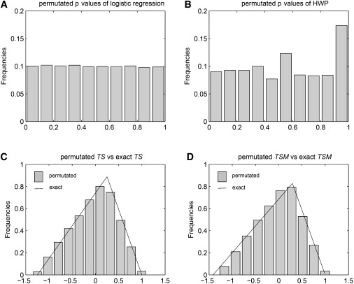
Permutated p Values and Permutated versus Exact TS and TSM Values under the Null Hypothesis

Web Resources

The URLs for data presented herein are as follows:

• Computing program, http://www.epigenetic.org/software.php

• Online Mendelian Inheritance in Man (OMIM), http://www.ncbi.nlm.nih.gov/Omim/

References

- 1.Engels E.A., Wu X., Gu J., Dong Q., Liu J., Spitz M.R. Systematic evaluation of genetic variants in the inflammation pathway and risk of lung cancer. Cancer Res. 2007;67:6520–6527. doi: 10.1158/0008-5472.CAN-07-0370. [DOI] [PubMed] [Google Scholar]
- 2.Sellers T.A., Vachon C.M., Pankratz V.S., Janney C.A., Fredericksen Z., Brandt K.R., Huang Y., Couch F.J., Kushi L.H., Cerhan J.R. Association of childhood and adolescent anthropometric factors, physical activity, and diet with adult mammographic breast density. Am. J. Epidemiol. 2007;166:456–464. doi: 10.1093/aje/kwm112. [DOI] [PubMed] [Google Scholar]
- 3.Scott L.J., Mohlke K.L., Bonnycastle L.L., Willer C.J., Li Y., Duren W.L., Erdos M.R., Stringham H.M., Chines P.S., Jackson A.U. A genome-wide association study of type 2 diabetes in Finns detects multiple susceptibility variants. Science. 2007;316:1341–1345. doi: 10.1126/science.1142382. [DOI] [PMC free article] [PubMed] [Google Scholar]
- 4.Hunter D.J., Kraft P., Jacobs K.B., Cox D.G., Yeager M., Hankinson S.E., Wacholder S., Wang Z., Welch R., Hutchinson A. A genome-wide association study identifies alleles in FGFR2 associated with risk of sporadic postmenopausal breast cancer. Nat. Genet. 2007;39:870–874. doi: 10.1038/ng2075. [DOI] [PMC free article] [PubMed] [Google Scholar]
- 5.Thomas G., Jacobs K.B., Yeager M., Kraft P., Wacholder S., Orr N., Yu K., Chatterjee N., Welch R., Hutchinson A. Multiple loci identified in a genome-wide association study of prostate cancer. Nat. Genet. 2008;40:310–315. doi: 10.1038/ng.91. [DOI] [PubMed] [Google Scholar]
- 6.Kozyrev S.V., Abelson A.K., Wojcik J., Zaghlool A., Linga Reddy M.V., Sanchez E., Gunnarsson I., Svenungsson E., Sturfelt G., Jonsen A. Functional variants in the B-cell gene BANK1 are associated with systemic lupus erythematosus. Nat. Genet. 2008;40:211–216. doi: 10.1038/ng.79. [DOI] [PubMed] [Google Scholar]
- 7.Poynter J.N., Figueiredo J.C., Conti D.V., Kennedy K., Gallinger S., Siegmund K.D., Casey G., Thibodeau S.N., Jenkins M.A., Hopper J.L. Variants on 9p24 and 8q24 are associated with risk of colorectal cancer: results from the Colon Cancer Family Registry. Cancer Res. 2007;67:11128–11132. doi: 10.1158/0008-5472.CAN-07-3239. [DOI] [PubMed] [Google Scholar]
- 8.Cheung C.L., Chan V., Kung A.W. A differential association of ALOX15 polymorphisms with bone mineral density in pre- and post-menopausal women. Hum. Hered. 2008;65:1–8. doi: 10.1159/000106057. [DOI] [PubMed] [Google Scholar]
- 9.Graffelman J., Camarena J.M. Graphical tests for HW equilibrium based on the ternary plot. Hum. Hered. 2008;65:77–84. doi: 10.1159/000108939. [DOI] [PubMed] [Google Scholar]
- 10.Gomes I., Collins A., Lonjou C., Thomas N.S., Wilkinson J., Watson M., Morton N. HW quality control. Ann. Hum. Genet. 1999;63:535–538. doi: 10.1017/S0003480099007824. [DOI] [PubMed] [Google Scholar]
- 11.Tapper W., Collins A., Gibson J., Maniatis N., Ennis S., Morton N.E. A map of the human genome in linkage disequilibrium units. Proc. Natl. Acad. Sci. USA. 2005;102:11835–11839. doi: 10.1073/pnas.0505262102. [DOI] [PMC free article] [PubMed] [Google Scholar]
- 12.Hosking L., Lumsden S., Lewis K., Yeo A., McCarthy L., Bansal A., Riley J., Purvis I., Xu C.F. Detection of genotyping errors by HW equilibrium testing. Eur. J. Hum. Genet. 2004;12:395–399. doi: 10.1038/sj.ejhg.5201164. [DOI] [PubMed] [Google Scholar]
- 13.Weir B.S. Sinauer Associates; Sunderland, Mass: 1996. Genetic data analysis II methods for discrete population genetic data. [Google Scholar]
- 14.Feder J.N., Gnirke A., Thomas W., Tsuchihashi Z., Ruddy D.A., Basava A., Dormishian F., Domingo R., Ellis M.C., Fullan A. A novel MHC class I-like gene is mutated in patients with hereditary haemochromatosis. Nat. Genet. 1996;13:399–408. doi: 10.1038/ng0896-399. [DOI] [PubMed] [Google Scholar]
- 15.Nielsen D.M., Ehm M.G., Weir B.S. Detecting marker-disease association by testing for HW disequilibrium at a marker locus. Am. J. Hum. Genet. 1998;63:1531–1540. doi: 10.1086/302114. [DOI] [PMC free article] [PubMed] [Google Scholar]
- 16.Jiang R., Dong J., Wang D., Sun F.Z. Fine-scale mapping using HW disequilibrium. Ann. Hum. Genet. 2001;65:207–219. doi: 10.1017/S0003480001008570. [DOI] [PubMed] [Google Scholar]
- 17.Czika W., Weir B.S. Properties of the multiallelic trend test. Biometrics. 2004;60:69–74. doi: 10.1111/j.0006-341X.2004.00166.x. [DOI] [PubMed] [Google Scholar]
- 18.Wittke-Thompson J.K., Pluzhnikov A., Cox N.J. Rational inferences about departures from HW equilibrium. Am. J. Hum. Genet. 2005;76:967–986. doi: 10.1086/430507. [DOI] [PMC free article] [PubMed] [Google Scholar]
- 19.Taylor J., Tibshirani R. A tail strength measure for assessing the overall univariate significance in a dataset. Biostatistics. 2006;7:167–181. doi: 10.1093/biostatistics/kxj009. [DOI] [PubMed] [Google Scholar]
- 20.Guo S.W., Thompson E.A. Performing the exact test of HW proportion for multiple alleles. Biometrics. 1992;48:361–372. [PubMed] [Google Scholar]
- 21.Wigginton J.E., Cutler D.J., Abecasis G.R. A note on exact tests of HW equilibrium. Am. J. Hum. Genet. 2005;76:887–893. doi: 10.1086/429864. [DOI] [PMC free article] [PubMed] [Google Scholar]
- 22.Benjamini Y., Hochberg Y. Controlling the False Discovery Rate - A Practical and Powerful Approach to Multiple Testing. J. Roy. Stat. Soc. B Met. 1995;57:289–300. [Google Scholar]
- 23.Spitz M.R., Hong W.K., Amos C.I., Wu X., Schabath M.B., Dong Q., Shete S., Etzel C.J. A risk model for prediction of lung cancer. J. Natl. Cancer Inst. 2007;99:715–726. doi: 10.1093/jnci/djk153. [DOI] [PubMed] [Google Scholar]
- 24.Shopland D.R., Eyre H.J., Pechacek T.F. Smoking-attributable cancer mortality in 1991: is lung cancer now the leading cause of death among smokers in the United States? J. Natl. Cancer Inst. 1991;83:1142–1148. doi: 10.1093/jnci/83.16.1142. [DOI] [PubMed] [Google Scholar]
- 25.Lethbridge-Cejku M., Schiller J.S., Bernadel L. Summary health statistics for U.S. adults: national health interview survey, 2002. Vital Health Stat. 2004;10:1–151. [PubMed] [Google Scholar]
- 26.Harber P., Tashkin D.P., Simmons M., Crawford L., Hnizdo E., Connett J. Effect of occupational exposures on decline of lung function in early chronic obstructive pulmonary disease. Am. J. Respir. Crit. Care Med. 2007;176:994–1000. doi: 10.1164/rccm.200605-730OC. [DOI] [PMC free article] [PubMed] [Google Scholar]
- 27.Cassidy A., Myles J.P., van Tongeren M., Page R.D., Liloglou T., Duffy S.W., Field J.K. The LLP risk model: an individual risk prediction model for lung cancer. Br. J. Cancer. 2008;98:270–276. doi: 10.1038/sj.bjc.6604158. [DOI] [PMC free article] [PubMed] [Google Scholar]
- 28.Ramsey S.D., Yoon P., Moonesinghe R., Khoury M.J. Population-based study of the prevalence of family history of cancer: implications for cancer screening and prevention. Genet. Med. 2006;8:571–575. doi: 10.1097/01.gim.0000237867.34011.12. [DOI] [PMC free article] [PubMed] [Google Scholar]
- 29.Cheng I., Plummer S.J., Casey G., Witte J.S. Toll-like receptor 4 genetic variation and advanced prostate cancer risk. Cancer Epidemiol. Biomarkers Prev. 2007;16:352–355. doi: 10.1158/1055-9965.EPI-06-0429. [DOI] [PubMed] [Google Scholar]
- 30.Neumann A.S., Lyons H.J., Shen H., Liu Z., Shi Q., Sturgis E.M., Shete S., Spitz M.R., El-Naggar A., Hong W.K. Methylenetetrahydrofolate reductase polymorphisms and risk of squamous cell carcinoma of the head and neck: a case-control analysis. Int. J. Cancer. 2005;115:131–136. doi: 10.1002/ijc.20888. [DOI] [PubMed] [Google Scholar]
- 31.Keith S.W., Wang C., Fontaine K.R., Cowan C.D., Allison D.B. BMI and headache among women: results from 11 epidemiologic datasets. Obesity (Silver Spring) 2008;16:377–383. doi: 10.1038/oby.2007.32. [DOI] [PMC free article] [PubMed] [Google Scholar]
- 32.Ruano-Ravina A., Figueiras A., Barros-Dios J.M. Type of wine and risk of lung cancer: a case-control study in Spain. Thorax. 2004;59:981–985. doi: 10.1136/thx.2003.018861. [DOI] [PMC free article] [PubMed] [Google Scholar]
- 33.Escabias M., Aguilera A.M., Valderrama M.J. Functional PLS logit regression model. Comput. Stat. Data Anal. 2007;51:4891–4902. [Google Scholar]
- 34.David H.A. Wiley; New York: 1981. Order Statistics. [Google Scholar]