Matchings and phylogenetic trees

Abstract

This paper presents a natural coordinate system for phylogenetic trees using a correspondence with the set of perfect matchings in the complete graph. This correspondence produces a distance between phylogenetic trees, and a way of enumerating all trees in a minimal step order. It is useful in randomized algorithms because it enables moves on the space of trees that make random optimization strategies “mix” quickly. It also promises a generalization to intermediary trees when data are not decisive as to their choice of tree, and a new way of constructing Bayesian priors on tree space.

Motivation

Much of the current research effort in phylogenetic methodology is being done in the exploration of Tree Space, the space of all phylogenetic trees with a given number of leaves n.e

Both the parsimony and maximum likelihood criteria lead to intractable combinatorial optimization problems on this space.f Validation of the tree obtained by such algorithms is hampered by the discreteness and complexity of this underlying space. Efforts to visualize the space have used graphs with vertices that are the possible trees and edges connecting trees that differ by a moveg of some sort. Most optimization algorithms use randomized moves that try to find local optima, using multiple starting points. Others follow the simulated annealing approach to randomized optimization; these also use random moves. A notion of neighborhood in this space would be most useful for inferential purposes.

Here, we introduce a bijection known to combinatorialists that allows construction of a coordinate system for phylogenetic trees. This system also admits a continuous interpolation, thus suggesting a way of making continuous confidence statements such as those provided by consensus of bootstraps or other resampling or perturbation methods. Finally, it allows the wealth of tools developed to study matchings (3) to be used for phylogenetic trees.

This coordinate system provides a new set of natural moves on the trees, providing at the same time distances in tree space and either a way of doing complete enumeration by going through all the trees in a step-by-step way or a means for doing a random walk on tree space. These are useful for doing simulated annealing for optimization. It is still an open problem to say how fast such a method would converge within a certain percentage of the optima; however, some progress is currently being made by the authors on the convergence to the uniform distribution for simple random walk (unpublished work).h

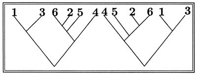
A phylogenetic tree is a binary rooted tree with n labeled leaves (see Fig. 1).i

Figure 1.

These two trees are considered identical.

Combinatorialists have known since 1870 that there are more than an exponential number of such trees (5).j Another recent proof of this result identifies phylogenetic trees with perfect matchings on (2n − 2) points (7).

What Is a Perfect Matching?

A perfect matching on 2m points is a pairing of the points into m groups of two—the order within a group or between groups does not matter. Here is a perfect matching on 10 points: (1, 4)(2, 10)(3, 6)(5, 9)(7, 8). It is easy to see there are (2m − 1)(2m − 3) … 3 perfect matchings on 2m points (so for m = 3 there are 15). There is a natural bijection, which assigns a matching of 2m points to a tree with m + 1 labeled leaves. Here is how the bijection is created (see Fig. 2).

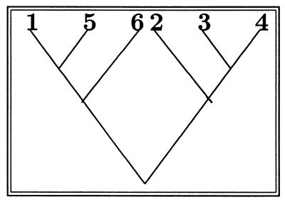
Figure 2.

An initial phylogenetic tree with the leaves relabeled as numbers. Here there are 6 = m + 1 leaves.

The first step is the labeling of ancestors.

• Look at all of the sibling pairs already labeled [here it is (1, 5) and (3, 4)].

• Choose the pair with the smallest child [which is (1, 5) in this example].

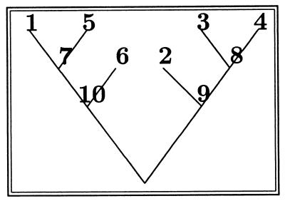
• Label that pair’s parent with the next available label (7 is put on the node ancestral to 1 and 5).

• Repeat until all ancestral nodes except the root are labeled (see Fig. 3).

Figure 3.

The tree of Fig. 2 with internal nodes labeled.

One now goes from this labeled tree to the matching, by pairing off the siblings: (1, 5)(3, 4)(6, 7)(2, 8)(9, 10).

In the other direction, we build a tree from a matching on 2m points. First we recall that the tree will have m + 1 leaves so that among all the sibling pairs in the matching there will be at least one that is made up only of leaves. If there are several, we choose the pair with the smallest child; this pair will be the first sibling pair (or clade) written down in the tree.

Here is an example: (1, 3)(2, 6)(5, 8)(4, 9)(7, 10). There are m = 5 pairs, so there will be 6 leaves labeled from 1 to 6, the first available ancestral label is 7. The labeled sibling pairs we start with are (1, 3) and (2, 6), of which (1, 3) has the smaller child, so it is assigned the parent 7; then the next labeled pair is (2, 6), and we assign it the next ancestor, thus building the tree sequentially. In the end we obtain the tree of Fig. 1. This is not the only bijection that can be constructed between perfect matchings and phylogenetic trees.k Several rules are possible for labeling the ancestors; for instance, we chose one that is easy to follow on the tree.

Comparison to the Existing Notation.

Biologists standardized their representation of trees by using a one-line parenthesized expression called the New Hampshire or Newick format.l The matching notation can be enriched the same way the Newick format enriches the parenthesis notation, so that the Newick tree with branch lengths is noted ((1 : 1, 4 : 1) : 3, ((2 : 1, 3 : 1), 5 : 2) : 1) and the corresponding matching notation would be (2 : 1, 3 : 1)(1 : 1, 4 : 1)(5 : 2, 7 : 1)(6 : 3, 8 : 1). There is still room outside the matching’s parentheses to add weights for each sibling pair.

Unfortunately the Newick notation is not a bijection; there are several such representations for the same tree.m But there is a simple algorithm for going from the Newick notation to the matching notation.n

Using Matchings to Build Distances in Tree Space.

Many distances proposed for measuring dissimilarities between trees are based on different ways of representing them. The correspondence with matchings allows comparisons based on methods used for permutations. For instance, one can count the number of transpositions needed to make one matching into another. To make (1, 4)(2, 6)(3, 5) into (2, 3)(4, 6)(1, 5), one needs to transpose 4 and 5, thus obtaining (2, 6)(3, 4)(1, 5), and then transpose 3 and 6. Thus two moves are necessary to transform the first matching into the second. For instance, the distance between the trees in Figs. 1 and 2 is four in this metric.

Counting the number of such moves between the two matchings gives a distance between trees that is easy to compute and is naturally invariant to irrelevant changes in labeling.o

The correspondence between matchings and trees opens up several new possibilities that are easy to visualize and compute in matching space. Here is a brief menu.

Gray Codes for Phylogenies.

Combinatorialists often seek ways of walking through the space of all objects in a step-by-step way. This is also useful for evaluating phylogenetic algorithms by running through all cases. The example treated shows how it is done with 4-leaved trees but the same method generalizes to any number of leaves.p

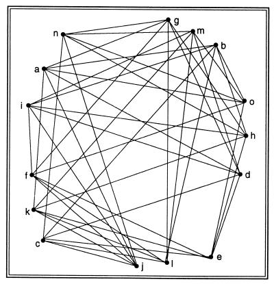
Fig. 4 shows all 15 trees on 4 leaves; two trees are connected if they are at distance one.

Figure 4.

The graph of all matchings on 6 points.

The problem at hand is to find a path through this graph that goes through each vertex once and once only; we will thus have enumerated all the trees from the first to the last with a minimal number of changes.q

Another enumeration scheme used on tree space (13) uses a branch and bound method for enumerating phylogenetic trees that make moves that are not always simple transpositions; therefore, it is not a Gray code in a reasonable sense.

Fourier Analysis in Tree Space.

Matchings admit a natural action of the permutation group which gives a spectral analysis for collections of trees. The group theory also allows analysis of the natural random walk on trees corresponding to random transpositions in matching space (see also ref. 4).

Relaxing the Matchings to the Polytope.

It is also the case that neither direct use of trees nor the parenthesis notation enables a representation in a continuous space. This has been a main problem in systematics for questions such as the following:

1.

How near to being tree-like are the data?

2.

Can the data be seen as indicating a mixture of several trees in some sense?

3.

How can one decompose the data into the best tree, the second best, etc., in a unique way so that, for instance, if there is a big difference between the first and second tree, this difference can indicate a preference for the first tree.

4.

How can one create nonparametric Bayesian priors on Tree Space?

If we take the convex hull of all the matchings on N points in the multidimensional space of dimension N(N − 1)/2, we obtain a polytope.r Any convex combination of trees gives a unique point in the polytope; thus the output from multiple runs of a tree building program can be summarized by a point in the polytope. Some points in the polytope can be represented in several ways as a convex combination of the vertices (possible trees). This is a way of summarizing a run from an optimizing procedure that ends in several optimal trees; instead of writing each tree in parenthesis notation, we can associate the point in the polytope, listing the closest trees and thus the coefficients in the matching polytope.

Randomized Algorithms for Optimization.

Several random heuristic methods are used for finding the optimal tree in some sense; these methods are based on random moves and an annealing schedule. A different method maintains a set of potential trees, choosing two at random and creating two new trees through a tree-reproduction scheme.t Algebraists have introduced a method for making a product of two matchings in what is known as the Brauer algebra (18, 19). This enables a simple implementation of a genetic algorithm; it remains an open problem to prove how fast, and under what conditions, this will converge to an optimum.

A Space Where Bayesian Nonparametrics Are Possible?

Several recent efforts of incorporating prior information about trees have been proposed (20–22). Unfortunately, all of these efforts have relied heavily on parametric models. The coordinate system suggested here enables other priors, for instance, priors could be set on the polytope as a whole with high probabilities for the vertices because biologists do believe in the prior postulate of an evolutionary tree.

All three implementations rely on Monte Carlo Markov Chains on Tree Space to compute the posterior probabilities; using the transposition moves on matchings will certainly simplify some of the computational technicalities.u

References

- 1.Foulds L R, Graham R L. Adv Appl Math. 1982;3:43–49. [Google Scholar]
- 2.Waterman M S, Smith T F. J Theor Biol. 1978;73:789–800. doi: 10.1016/0022-5193(78)90137-6. [DOI] [PubMed] [Google Scholar]
- 3.Lovasz L, Plummer M D. Matching Theory. Amsterdam: North–Holland; 1985. [Google Scholar]
- 4.Diaconis P, Hanlon P. Contemp Math. 1992;138:99–117. [Google Scholar]
- 5.Schröder E. Z Math Phys. 1870;15:361–376. [Google Scholar]
- 6.Cavalli-Sforza L L, Edwards A W F. Evolution. 1967;21:550–570. doi: 10.1111/j.1558-5646.1967.tb03411.x. [DOI] [PubMed] [Google Scholar]
- 7.Stanley R. Enumerative Combinatorics. II. Cambridge, U.K.: Cambridge Univ. Press; 1998. [Google Scholar]
- 8.Erdös P L, Székely L A. Adv Appl Math. 1989;10:488–496. [Google Scholar]
- 9.Felsenstein J. phylip(Phylogeny Inference Package) University of Washington, Seattle: Department of Genetics; 1993. , Version 3.5c. [Google Scholar]
- 10.Critchlow D E. Metric Methods for Analyzing Partially Ranked Data, Lecture Notes in Statistics. New York: Springer; 1985. [Google Scholar]
- 11.Gray F. Bell Systems Technical Journal. 1939;18:252. [Google Scholar]
- 12.Diaconis P W, Holmes S P. Stat Comput. 1994;4:287–302. doi: 10.1007/s11222-015-9562-9. [DOI] [PMC free article] [PubMed] [Google Scholar]
- 13.Hendy M D, Penny D. Math Biosci. 1981;59:277–290. [Google Scholar]
- 14.Dress A, Krüger M. Adv Appl Math. 1987;8:8–37. [Google Scholar]
- 15.Barker D. LVB 1.0: Reconstructing Evolution with Parsimony and Simulated Annealing. Edinburgh: Daniel Barker; 1997. http://www.icmb.ed.ac.uk/sokal.html (available at http://www.icmb.ed.ac.uk/sokal.html). ). [Google Scholar]
- 16.Matsuda H. In: Pacific Symposium on Biocomputing. Hunter L, Klein T E, editors. London: World Scientific; 1996. pp. 512–523. [Google Scholar]
- 17.Lewis P O. Mol Biol Evol. 1998;15:277–283. doi: 10.1093/oxfordjournals.molbev.a025924. [DOI] [PubMed] [Google Scholar]
- 18.Brauer R. Ann Math. 1937;38(2):857–872. [Google Scholar]
- 19.Hanlon P, Wales D. J Algebra. 1989;121:446–476. [Google Scholar]
- 20.Li, S., Pearl, D. K. & Doss, H. (1999) J. Am. Stat. Assoc., in press.
- 21.Mau, B., Newton, M. A. & Larget, B. (1999) Biometrics, in press. [DOI] [PubMed]
- 22.Yang Z, Rannala B. Mol Biol Evol. 1997;14:717–724. doi: 10.1093/oxfordjournals.molbev.a025811. [DOI] [PubMed] [Google Scholar]
- 23.The MathWorks, Inc. matlab. Inc., Natick, MA: The MathWorks; 1997. , Version 5. [Google Scholar]