

Abstract
Evaporation is a well known issue when handling small liquid volumes. Here we present a review of microscale assays prone to evaporation and methods to make them more robust. Applications for these assays span from combinatorial chemistry to cell-biology where the stability of concentrations and osmolarity can be critical. A dimensionless evaporation number Ev is presented and used to characterize volume loss in short term and long term microscale assays. Ev can be used both as a design tool and as an analysis parameter. The advantageous use of evaporation in some applications is also discussed.
Introduction
Microfluidics stems from the realization that reducing device sizes induces a range of benefits in terms of speed, cost, and precision.1 Beyond these advantages, new functionality arises including the ability to analyze single cells or even single molecules through control of extremely small volumes and the ability to run these experiments in parallel in an array based format.2–5 Many approaches to manipulate volumes down to the picoliter scale have been devised to create microfluidic devices.6
One approach consists of limiting the dead volume by removing tubes and connectors, which will be referred to here as tubeless microfluidics. A first category of such devices maintains the concept of microchannels. To generate flow they rely on passive phenomena such as surface tension7–9 or integrated actuators as in electrowetted flow.10 These tubeless microfluidic devices allow integration of most existing microfluidic functions such as valves and reaction chambers.
Reducing the volumes further, a second category of devices discard the concept of flow and microchannels, to reduce the reaction and detection chambers to a single drop of liquid. Micro and nano vial arrays enable the creation of thousands of parallel reaction chambers.11–16 Electrowetting on dielectric (EWOD) allows the operations of creating, displacing, fusing and detecting drops of fluid.17,18
Devices such as EWOD (Fig. 1B) and passive pumping chips (Fig. 1C) allow on-chip manipulation of the fluid once dispensed. While nanovial arrays (Fig. 1A) do not offer this capability, they are a promising approach to combinatorial chemical synthesis. All these devices share two main characteristics. They eliminate the requirement for liquid connectors using other dispensing devices such as pipettors7,19 or inkjet printers20 instead. Moreover, they are all based on droplet dispensing to create arrayable small work volumes.
Fig. 1.

Example of microfluidic devices presenting open air–liquid interfaces susceptible to evaporation. A: Nanovial arrays. B: EWOD chip.17 C: Passive pumping chip.
One of the critical issues in using this class of microfluidic device is evaporation due to the open air–liquid interfaces.21 The subsequent volume loss affects the concentrations and osmolarity of reagents or media. For perspective, in typical laboratory conditions a 10 nL drop will evaporate in 10–30 s.22 Volume loss is exacerbated for experiments lasting hours or days, such as cell studies, increasing its importance as an experimental parameter.
There are many approaches to reducing the effects of evaporation. The time scale of the experiment can be reduced by parallelizing the dispensing of liquid and detection methods.11 The evaporation rate can be reduced by changing the geometry of the device and reducing the ratio of exposed area to volume.12 A high boiling point component (e.g. glycerol in the case of aqueous working fluids) can be added to the liquid to reduce the vapor pressure, provided it does not modify the function of the assay.23
More sustainable solutions are required for experiments such as cell studies lasting up to a few days. First, the evaporation can be compensated for by continuous addition of liquid to the depleted reservoir.14,24 In addition to the effects of flow, this approach adds to the complexity of the fabrication and may cause changes in solute concentration.
Another technique is to block any open gas–liquid interface. Mineral oil is typically used to cap exposed aqueous solvents,5,15,16 or heptane for easier removal,6 preventing evaporation of the underlying water but reducing the ease of access to the liquid compartments. The system can also be isolated by using solid lids such as a microscope slide.22
Finally, perhaps the most commonly used method is to place the microfluidic device in a closed humid environment. This can be done by placing sacrificial water around the liquid of interest in a closed container. Drawbacks include unwanted condensation in the presence of temperature gradients and hindered/limited device access. However, creating a humid environment is the least invasive method as it minimizes interaction with the fluid of interest. Thus, this method will be the focus of further characterization.
While this solution is often successful, it is typically empirical and relies on the assumption that the level of humidity provided is sufficient to mitigate evaporation. In some cases, as devices become denser and the user wishes to use specialized equipment with space constraints (e.g. a microscope stage, mass spectrometer, etc.), it is impossible to deposit liquid in the same manner. A design parameter to ensure acceptable evaporation is needed.
In this tutorial review, we begin with the analysis of an evaporating surface. This allows us to write the evaporation rate of different geometries, such as droplets or disks. For medium to high throughput microfluidic applications involving liquid–air interfaces, we introduce a dimensionless number, Ev, quantifying the fractional volume loss through evaporation of a liquid of interest in the presence of sacrificial liquid. Design solutions for a range of situations and liquids are presented and discussed. Finally, specific considerations are analyzed, such as the modified evaporation rate for high array of large number and edge effects, which can lead to significant changes in evaluating evaporation.
Theory
Evaporation is a diffusion limited process of water vapor moving away from the air–liquid interface depending on the surrounding conditions such as mass concentration of water vapor, C (kg m−3), or temperature.25,26 The evaporation rate, E, written in terms of D, the diffusion coefficient of water vapor in air, ρ, the density of water, and n a unit vector normal to the interface,27 is given by:
| (1) |
Analytical solutions for the evaporation process are nontrivial, however the problem can be simplified if we suppose temperature to be constant.28 For still air, a concentration gradient of vapor develops by diffusion,29,30 and the concentration difference between the surface of the interface and the air is written ΔCsat-i. Note that a ventilated environment increases evaporation rates.31
In the case of a hemispherical droplet of radius R, the gradient of vapor concentration takes a value of ΔCsat-i/R at the interface and the evaporation rate is written in eqn (2).29,32 The general case of a droplet on a surface can be approximated with knowledge of the contact angle (see ESI‡). Interestingly, the evaporation rate is proportional to the radius and not the surface area of a drop:
| (2) |
An exact solution for steady-state evaporation for a flat disk can be written, by using an equivalent radius in eqn (2), where S is the surface area.33 More generally, for qualitative purposes, this solution can be extended to compact shapes of surface area S:
| (3) |
For different liquids, the evaporation rate is modified depending on their saturated vapor pressure, which can be written as a function of osmolarity (see ESI‡). Eqn (1)–(3) allow us to pursue the quantification of the volume loss in an assay containing sacrificial liquid.
Evaporation number
It is possible to approach the problem of evaporation in a container from a general perspective, without considering the evaporation for each single source. During an experiment a volume, V loss, is lost through evaporation in the whole device, resulting in changes in concentrations and osmolarity. For example, after the liquid of interest (e.g. cell suspension or reagent) and the sacrificial liquid are placed in a chamber, the vapor pressure rises to equilibrate near saturation leading to a loss in liquid volume, V ini. Continuous volume loss, V leak, also occurs by diffusion through leaks, of influx of drier gases (e.g. CO2 in an incubator):
| (4) |
Volume loss will occur both in the liquid of interest, which we wish to minimize, and in sacrificial liquid (Fig. 2). The sum of evaporation rates at the surfaces of interest, Ei, calculated using eqn (2) or (3), is the amount of unwanted evaporation. The sum over all sources represents the total evaporation rate. The ratio of these sums represents the fraction of evaporation of interest, ξ:
| (5) |
Fig. 2.
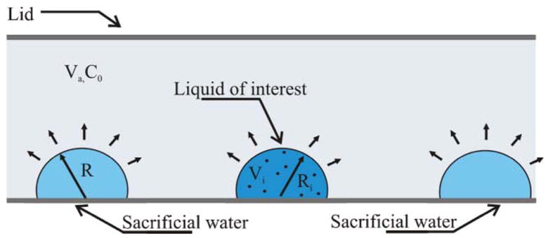
Parameters in the evaporation number Ev and Evini. The liquid is placed in a container of volume V a at a humidity C0. Drop k of volume V k has a radius of Rk.
From eqn (2), (4) and (5) we evaluate the volume of the liquid of interest evaporated. By comparing this volume to the total volume of the liquid of interest initially placed in the container, V i, the fraction of liquid of interest lost, Ev, can be evaluated. In this form Ev can also be split into evaporation numbers specific for each phenomenon, such as Evini, for initial evaporation, and Evleak for continuous loss:
| (6) |
The acceptable threshold for Ev depends on the requirements of a particular experiment. For mouse embryos, osmolarity changes of more than 5% can modify their development.34 In this case Ev must be well under 0.05. In different conditions higher Ev may be acceptable.
In the following, we will focus the case study on an array of drops as they are easily dispensed using a micropipette (Fig. 2 and 3), thus eqn (5) and (6) are rewritten in eqn (7) with R the radius of the drop and Ri, the radius of the drop of interest. However, for shapes that are not too elongated, the equivalent radius presented in eqn (3) can be used. This is demonstrated in an application presented in the closure of this analysis. The different contributions to Ev are evaluated depending on the situation.
Fig. 3.
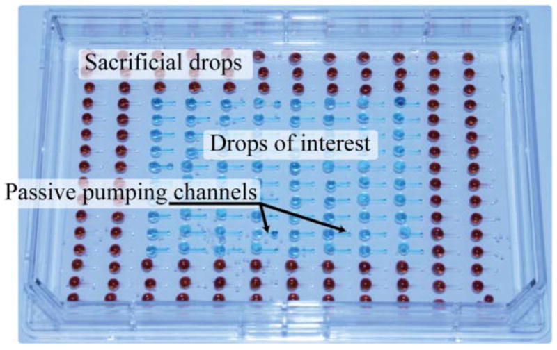
Experimental passive pumping based assay in an open Omnitray containing both drops of liquid of interest and sacrificial drops that will reduce volume loss on the drops of interest.
| (7) |
Short term volume loss
The initial evaporation leads to a rise in humidity in the container to reach near saturated conditions. For example, we measured that equilibrium is reached in 15 minutes in a 90 mL closed Omnitray (NUNC, Rochester, NY) at 25 °C containing one hundred 10 μL drops (Fig. 4 and ESI‡). For a container of volume Va, the total amount of volume loss corresponds to the volume of water required to saturate the air of the container. Thus, we write the evaporation number, Evini, for the initial evaporation:
| (8) |
Fig. 4.
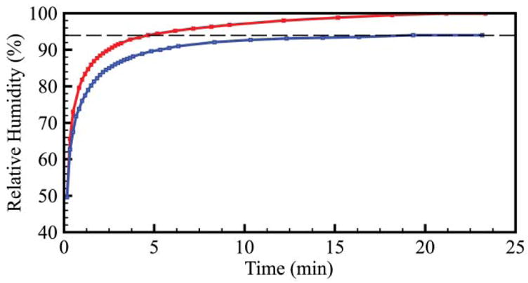
Humidity equilibration in a parafilm-sealed Omnitray (top line) and in a closed Omnitray (bottom line).
In the ideal case of a sealed and homogenous chamber, eqn (8) is sufficient to predict evaporation in long term experiments. However, the presence of leaks in the chamber leads to continuous volume loss that requires further analysis.
Long term volume loss
Measurement of the humidity equilibration (Fig. 4) reveals that the relative humidity (RH) in a closed but unsealed Omnitray equilibrates to 95% when ambient air is at 50% relative humidity (RH), signifying a continuous loss of humidity. This volume loss can be dominant for long term experiments, such as cell culture. If the leak flux J (in m3 s−1) is known, the total volume loss is JΔt for an experiment lasting a time Δt. EvLeak is given by:
| (9) |
In many cases, the leak is driven by diffusion through a concentration drop from the interior of the container to the exterior, ΔCi–e. Generally for small leaks, humidity in the container can be considered saturated and ΔCi–e ≈ ΔCsat-e. For these leaks, we write the leak rate J in the form of a diffusion process, with D the diffusion coefficient of water in air and ζ a geometric factor that represents the leakiness of a container. Alternatively, the parameter 1/Dζcan be viewed as the diffusive resistance with units s m−3:
| (10) |
A large value of ζ indicates strong leaks and a small value indicates a good seal. For simple geometries ζ can be calculated analytically. If the leak was driven by a straight channel of section A and length ℓ, ζ = A/ℓ. In general, for a random container of complex geometry, ζ can be determined experimentally using a simple protocol. First the user should time the duration for total evaporation of a known volume, V tot, from a container of interest. Total evaporation occurs for an Ev of 1, thus using eqn (10), ζ can be calculated:
| (11) |
Values of ζ have been determined experimentally for various containers commonly used in cell culture (Table 1). We notice an increase in the leakiness, ζ, for larger container perimeters and looser lids. With an expression for the leak rate, it is possible to determine the equilibration humidity in the container. At equilibrium, total evaporation in the container is summed using eqn (2), and equates to the water vapor leak, driven by diffusion out of the container. Therefore, ΔCsat-i, the water vapor concentration difference between saturation and the air of the container is:
| (12) |
Table 1.
Characteristic leakiness factor ζ for different platforms with standard deviation determined using eqn (5) from experimental results (see ESI‡)
| Container | Perimeter | Leakiness ζ |
|---|---|---|
| Tissue culture flask (T50) | N/A | ζ= 0.6 +/−0.02 10−3 m |
| Petridish 1″ | 79 mm | ζ= 2.5 +/−0.1 10−3 m |
| Petridish 2″ | 160 mm | ζ= 3.3 +/−0.3 10−3 m |
| Petridish 4″ | 315 mm | ζ= 4.9 +/−0.7 10−3 m |
| Omnitray closed | 430 mm | ζ= 6.5 +/−0.3 10−3 m |
| Omnitray sealed | 430 mm | ζ= 1.7 +/−0.2 10−3 m |
As an example, to verify Ev, a series of experiments were conducted. A number of identical 10 μL drops, one of which represents the “useful” drop, were placed in a 4″ Petridish at different temperature conditions for 6 h (Fig. 5). The weight variation of the device was measured to characterize the amount of evaporation that occurred. The Ev number was evaluated using eqn (6) with the geometric factor ζ calculated with eqn (11) and the water vapor concentration evaluated using the absolute water concentration at room conditions (21°, 20% RH). An Ev of 1 or more always indicated total evaporation of the liquid of interest. Evaporation of less than 10% always occurred for Ev numbers less than 0.1, whereas evaporation of more than 25% occurred for Ev numbers higher than 0.25 (Fig. 5). We note that Ev is not a highly precise measure of the amount of evaporation, due mainly to the uncertainty in measuring ζ, but produces sufficient quantification for the purpose of designing low evaporation experiments. Moreover, phenomena such as edge effects or interaction between evaporating sources have not been considered in this analysis.
Fig. 5.
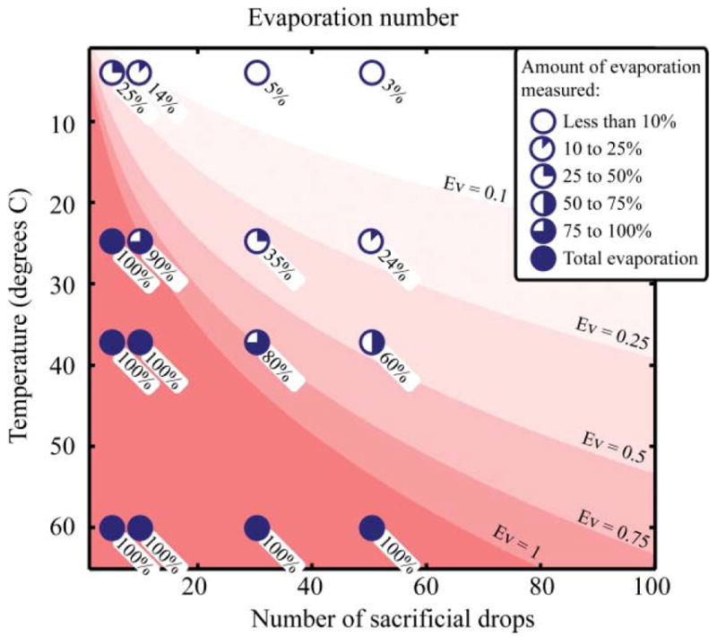
Evaporation numbers in a 4′ Petridish for a different number of sacrificial drops with one drop of interest at different temperatures but for the same absolute humidity concentration (concentration at 2° and 20% RH). Shades of red show increasing Ev numbers. Experimental data points and the measured fraction of evaporation are plotted with pie charts with the exact measured amount specified below.
Condensation
Although evaporation can have acute effects by significantly reducing volumes, condensation can also occur to promote increases in fluid volumes. This has been observed, particularly in cell culture applications where media and buffer are typically at 300 milliosmolar. If pure water is used to increase humidity in a device, the difference in osmolarity can drive condensation of water into the media. Further it has also been hypothesized as the cause of significant cell death (data not published). The difference in osmolarity just described would result in a negative value for ΔC. Thus, previously developed equations would yield a negative value for Ev, signifying condensation. Similarly, temperature gradients can result in significant condensation.
Edge effects: Placing sacrificial liquid judiciously
As mentioned, a neglected factor in the preceding analysis is the importance of local effects. For example, it is common practice in the use of 96 well plates for drug screening to omit the first and last rows and columns of the plate due to variability caused by evaporation. Diffusion of water vapor not only limits the evaporation rate of the liquid but also the homogenization of the environment. This signifies that a local effect such as a leak or a hole in the container will affect the closest drop much more than the others. This phenomenon is dependent on the height of the container and generally not on the density of evaporating “spots”. We illustrated this by modeling in COMSOL a Petridish either filled with water (Fig. 6A1) or containing multiple drops (Fig. 6A2). We observe that, regardless of a continuous or discrete surface of liquid, the evaporation only affects liquid at a set distance inside the Petridish, except for very spare arrays. Moreover, the distance from the leak at which the liquid undergoes only 5% of the evaporation predicted by the Ev number is about 3 to 4 times the height of the container (Fig. 6B). This distance does not vary with humidity and varies little with the leakiness (i.e. the physical size of the leak, see ESI‡), as they are both included in the calculation of Ev. For example, if the humidity outside the dish is cut in half, the average evaporation and Ev will double, yet the penetration distance associated with 5% of Ev will not change. This implies that placing the sacrificial liquid strategically can reduce evaporation more effectively than a large quantity of poorly placed liquid. This is especially true in the case of shallow containers. We illustrated the importance of this effect experimentally through observation of the evaporation pattern of an array of drops in an Omnitray overnight. At any time the two rows of drops closer to the edge seem to undergo extensive evaporation while the rest remain untouched (Fig. 6C).
Fig. 6.
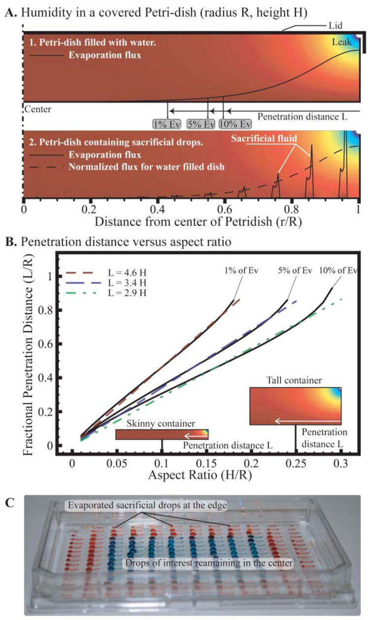
A. Humidity in a covered Petridish with a loose lid modeled in COMSOL with axisymetric geometry for both a dish filled with water (1) or containing an array of drops (2). The evaporation flux at the surface of the liquid is superposed and the distance, L, at which evaporation is reduced by x% is termed penetration distance. B. Penetration distance of the evaporation due to the leak as a fraction of the radius of the dish in function of the aspect ratio of the container. We observe that this distance is roughly proportional to the height of the container, and the coefficient depends on the percentage of evaporation reduction. C. Evaporation pattern in an Omnitray containing an array of passive pumping channels after 24 hours in room conditions with a lid. The 80 central channels are filled with blue colored water, and the 112 at the outskirts with red. This is the same device as in Fig. 3 after 24 h. If the leak spans the entire height of the dish, the penetration depth associated with 5% of Ev will be L = 2.3H + 0.03 (see ESI‡).
Evaporation for many arrayed sources
One hypothesis underlying the evaporation number is that each evaporating surface is far away enough from the others to neglect any interaction and thus, evaporation acts as if the surface was alone. In reality, for multiple drops, the fraction of evaporation will be reduced as they are more numerous on the same surface. This occurs because the area around the evaporative surface can no longer be considered as a semi-infinite space. This phenomenon becomes significant as the ratio of evaporating surface relative to the total surface of the assay increases. For sparse arrays, with a small ratio of areas, negligible direct interaction occurs between any pair of drops, yet the actual total evaporation rate is smaller than the sum of all individual evaporation rates. For this reason eqn (2) and (3), which are linear with N, need to be modified. Supposing an array of N evaporating surfaces of radii r, covering a disk-shaped area of substrate of radius a, we write the modified integrated evaporation rate, E in eqn (13a) and (13b). Eqn (13a) assumes that the evaporating sources are hemispherical, whereas eqn (13b) assumes disk-shaped surfaces33,35(see ESI‡):
| (13a) |
| (13b) |
We demonstrated this effect by measuring the evaporation of a number of disk shaped surfaces in a lidless 80 mm Petridish. The disks were created by floating a pierced plastic transparency sheet, bored using a 375 μm drill tip, on a Petridish filled with water and sealed with oil. The evaporation rate was measured by weighing the Petridish after 48 hours. As the holes in the transparency were not readily measurable and irregular in size, we estimated their diameter experimentally using the evaporation rate of 21 evenly distributed disks, supposing they still verified the low number hypothesis (Fig. 7A). The traditional model shows good accuracy for less than 100 disks; however, as the number of sources increases, it fails to predict the subsequent reduction in total evaporation. Rapidly the predicted evaporation rate intersects the measured total evaporation rate for the complete surface of the Petridish being liquid, highlighting the contradiction and limits of the traditional model. However, the evaporation rate was reduced in good coherence with eqn (13b). It is interesting to realize that the total evaporating surface was still small compared to the area of the Petridish, with a ratio of 0.0023 or 0.026, whether we used the estimated disk radius or the actual drill tip radius.
Fig. 7.
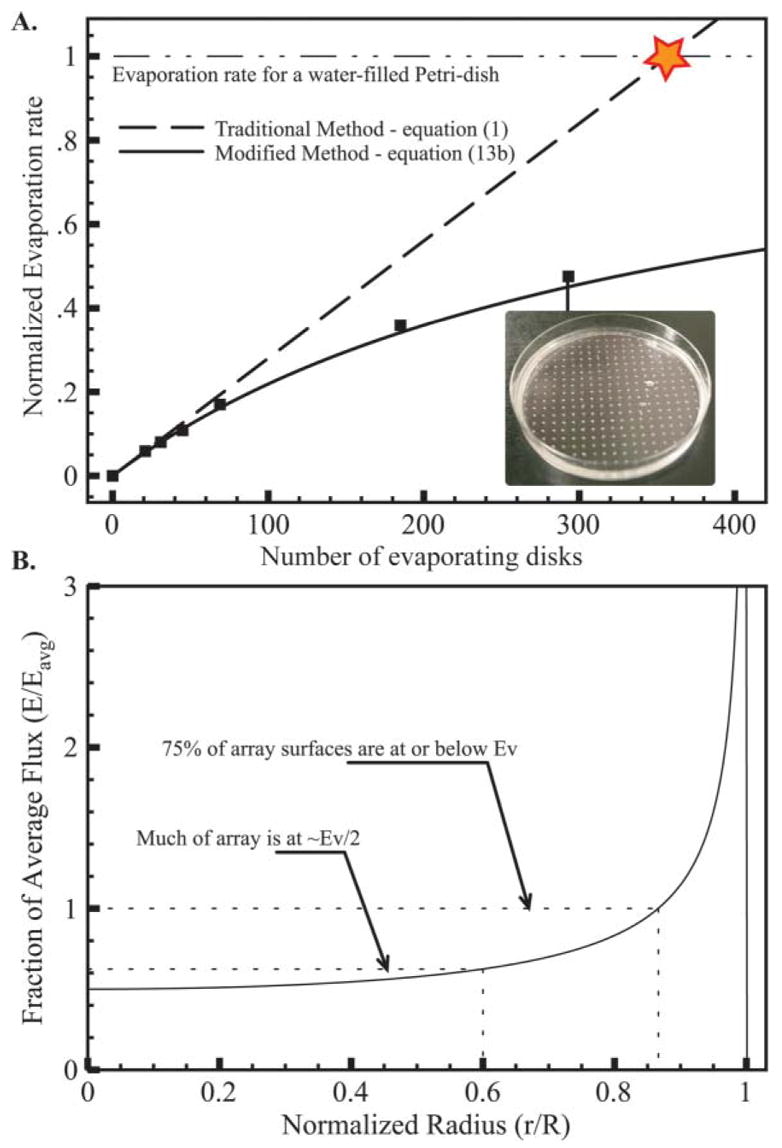
A. Total evaporation rate of an array of disk-shaped evaporating disks in a Petridish in function of their number. Experimental values (squares) are normalized by the evaporation rate for a whole evaporating Petridish filled with water. The average radius of the disks is found to be 112 μm using the evaporation rate of 21 disks and supposing the density effect is negligible. This value is used for plotting of the theoretical evaporation rates for both the traditional and modified model given by eqn (1) and eqn (13b) respectively. The maximum evaporation measured on a Petridish completely exposed is used to normalize these results and show the obvious contradiction of the traditional model. Note that even for 300 disks the distribution of the disks is sparse. B. Local evaporative flux from the center of the array out compared to the average flux. A slim band on the edge suffers severe evaporation whereas most of the array experiences less.
One of the assumptions of this calculation is that the volume of air around the assay is large such that it does not interfere with the evaporation process. For most containers, the lid will modify the humidity pattern and the evaporation will be defined by the leak rather than the liquid inside. For this reason we characterized this phenomenon by observing a lidless container. This modified evaporation model can be used for an assay during manipulation, when the lid is removed, or for assays done in large humid containers, such as incubators for instance. Furthermore, the overall concentration gradient driving the evaporation will be larger on the outskirts of the assay.36 Thus the center portion of the assay will experience roughly half the evaporation predicted by the Ev number (Fig. 7B).
When packing the drops or other evaporating surfaces in an even denser fashion, they will share their saturated humidity “halo” and act as a continuous liquid surface. This effect is progressively dominant as the ratio of evaporating surface to total surface increases. In this case, the evaporation rate for the whole device is given by eqn (2) and (3) with Req calculated for the whole surface of the array.
Applications
The knowledge of leaks and evaporation rates enables a controlled balance of each. To illustrate this we build a humidity controlled chamber using the balance of evaporation offered by a number of 1″ Petridishes filled with liquid, and the leak of a Bioassay Tray (NUNC, Rochester, NY). First the leakiness factor of the container, ζ, was determined using eqn (11) at room temperature. We then placed a number of Petridishes filled with water in the Tray and a humidity probe was inserted in the container. We measured the relative humidity at equilibrium after placing the tray in a dry incubator (Fig. 8). The experimental values follow the theory given by eqn (12) although we note that the measured humidity is generally higher than the expected theoretical value. We explain this by the edge effect previously mentioned, due to a ring of evaporation sources around the area of measurement.
Fig. 8.
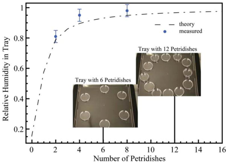
Humidity in a Bioassay Tray placed in an incubator at 37° and 10% relative humidity as a function of the number of Petridishes present inside. Theoretical values (dashed line) are found using eqn (12). Experimental values (dots) were measured for 3 configurations.
Discussion
In high-throughput screening and many applications of microfluidics, variation of volumes and osmolarity can affect the outcome of the experiment. The evaporation number integrates the analysis of evaporation for each evaporating surface to give a single comprehensive parameter to quantify this volume loss. Depending on the conditions, additional terms can be added to this number to account for the phenomena occurring during evaporation. Evini can be used alone in hermetically sealed containers, or for experimental times that are short compared to the equilibration time. Evleak, is used for long term experiments including contributions from leaks. Evleak necessitates the determination of the characteristic geometric factor, ζ, described with eqn (11). The evaporation number, Ev can be directly interpreted as the relative osmolarity or volume change. As a general rule, values of Ev under 0.1 signify that loss of volume through evaporation will be less than 10%.
The volume loss is also localized in the assay. Typically, leaks due to lids create a zone of higher evaporation extending in from the edge roughly 3 times the height of the container. This signifies that a thin container will experience a severe difference of evaporation between the center and the edge. Additionally we demonstrated that a continuous surface of liquid or discrete sacrificial surfaces do not effect the humidity profile. Therefore, although the punctual sources will deplete faster, it could be beneficial to apply the sacrificial sources at the same time and in the same format as the liquid of interest. Moreover, for repeatable experiments it is recommended not to use the locations close the boundaries. This edge effect phenomenon, referred to as the ‘sentinel effect’, also suggests that the closer to the ceiling the sacrificial liquid is placed the less dry air penetrates into the container. Additionally, two containers can be used to leverage the sentinel effect, by placing one inside the other. Fluid in the outer container humidifies air surrounding the inner container. In brief, determination of Ev provides an assessment of the magnitude of the evaporation supposing a random distribution of the liquids in the container. The characterization of the edge effects allows the modification of this Ev number to compensate for local variations in evaporation. For example, in the case of Fig. 3, the maximum Ev number for the drops is in fact 10% of the general Ev as the drops are at a minimum of 3 times the height of the tray away from the edge.
However, several factors have not been discussed. First, temperature gradients create an important amount of displacement of water through evaporation at warm spots and condensation at cooler spots. Experiments show that a 5 degree temperature gradient within a sealed Omnitray will cause the evaporation of one hundred 10 μL drops of water (1 mL) in less than 5 h (see ESI‡). This is typically very difficult for time-lapse imaging where light from a microscope creates localized heat. In general as temperature acts on every drop, no amount of sacrificial liquid can mitigate this phenomenon, and temperature gradients should be minimized. A possible mitigation of this phenomenon is to increase heat mixing of the air around the container through convection. A second limitation of this evaporation number resides in its consideration of only the initial state of the system. Therefore, when trying to minimize evaporation, Ev will remain accurate, since the system will not evolve much. However it cannot be used reliably to predict the state of the system for large evaporation.
Finally, although evaporation is seen as a problematic issue for most applications, it has been investigated for use in two main applications. The first application relies on a mechanism that is in part responsible for water flow in trees.37,38 This mechanism has been used to generate slow, steady, and long term flow in microchannels39–42 or for thin layer chromatography.43 Continuous flow rates down to 1 nL min−1 have been demonstrated to be considerably more stable than other external mechanical pumping systems.40 Furthermore, it has been shown that evaporation can be used to increase the concentration of an analyte of interest in a particular solution.11,44,45 This provides for a completely passive technique compared to the previous electrical field based or chemical gradient based methods. In addition, evaporation has been used to pack beads at the tip of a micropipette for biotechnological use.46
Conclusion
Important medical and biotechnological advances become possible with the ability to manipulate volumes of liquid of nanolitres or less in high-throughput form. Many approaches opt for tubeless microfluidic devices or droplet based microfluidics, thus reducing the handled volumes to a minimum. These small volumes, however, are acutely susceptible to volume loss through evaporation, especially over long periods of time.
Different solutions have been developed to mitigate evaporation. The most effective methods use lids that are either made of non-miscible fluids, such as oil, or are solid. For biological applications, another solution is to saturate the atmosphere using sacrificial water placed around the area of interest. For long term experiments, depending on the container, the duration of the experiment and the number of evaporating surfaces, the total volume loss can be determined, and the importance of evaporation quantified by the number Ev. Edge effects potentially modify evaporation and can be either a factor enhancing volume loss or a solution for mitigating it.
Here we analyzed only the immediate consequence of evaporation that is the loss of liquid volume and the subsequent concentration variations. Another consequence of evaporation is the generation of flows in the fluid, and the potential impact on the assay, particularly in the case of cell biology. This is the focus of a following analysis.47
Supplementary Material
Acknowledgments
This work was supported by funding from the MacDiarmid Institute for Advanced Materials and Nanotechnology (EB), the National Library of Medicine (JW–NLM #5T15LM007359) and NIH R21 #CA122672 and K25 #CA104162. Finally, the authors thank students and staff of the MMB Lab for their support and precious input.
Footnotes
For Part 2 see ref. 47.
Electronic supplementary information (ESI) available: Appendices I–V. See DOI: 10.1039/b717422e
Notes and references
- 1.Squires TM, Quake SR. Rev Mod Phys. 2005;77:977–1026. [Google Scholar]
- 2.Wikswo JP, Prokop A, Baudenbacher F, Cliffel D, Csukas B, Velkovsky M. IEE Proc–Nanobiotechnology. 2006;153:81–101. doi: 10.1049/ip-nbt:20050045. [DOI] [PubMed] [Google Scholar]
- 3.Lee SJ, Lee SY. Appl Microbiol Biotechnol. 2004;64:289–299. doi: 10.1007/s00253-003-1515-0. [DOI] [PubMed] [Google Scholar]
- 4.Hietpas PB, Ewing AG. J Liq Chromatogr. 1995;18:3557–3576. [Google Scholar]
- 5.Bratten CDT, Cobbold PH, Cooper JM. Anal Chem. 1997;69:253–258. [Google Scholar]
- 6.Gratzl M, Yi C. Anal Chem. 1993;65:2085–2088. [Google Scholar]
- 7.Walker GM, Beebe DJ. Lab Chip. 2002;2:131–134. doi: 10.1039/b204381e. [DOI] [PubMed] [Google Scholar]
- 8.Berthier E, Beebe DJ. Lab Chip. 2007;7:1275–1478. doi: 10.1039/b707637a. [DOI] [PubMed] [Google Scholar]
- 9.Meyvantsson I, Warrick J, Hayes S, Skoien A, Beebe DJ. Lab Chip. 2008;8 doi: 10.1039/b715375a. [DOI] [PubMed] [Google Scholar]
- 10.Satoh W, Hosono H, Suzuki H. Anal Chem. 2005;77:6857–6863. doi: 10.1021/ac050821s. [DOI] [PubMed] [Google Scholar]
- 11.Neugebauer S, Evans SR, Aguilar ZP, Mosbach M, Fritsch I, Schuhmann W. Anal Chem. 2004;76:458–463. doi: 10.1021/ac0346860. [DOI] [PubMed] [Google Scholar]
- 12.Mayer G, Kohler JM. Sens Actuators, A. 1997;60:202–207. [Google Scholar]
- 13.Litborn E, Emmer A, Roeraade J. Anal Chim Acta. 1999;401:11–19. [Google Scholar]
- 14.Litborn E, Emmer A, Roeraade J. Electrophoresis. 2000;21:91–99. doi: 10.1002/(SICI)1522-2683(20000101)21:1<91::AID-ELPS91>3.0.CO;2-Y. [DOI] [PubMed] [Google Scholar]
- 15.Litborn E, Roeraade J. J Chromatogr, B. 2000;745:137–147. doi: 10.1016/s0378-4347(00)00037-2. [DOI] [PubMed] [Google Scholar]
- 16.Clark RA, Hietpas PB, Ewing AG. Anal Chem. 1997;69:259–263. doi: 10.1021/ac970070x. [DOI] [PubMed] [Google Scholar]
- 17.Cho SK, Moon HJ, Kim CJ. J Microelectromech Syst. 2003;12:70–80. [Google Scholar]
- 18.Su F, Chakrabarty K, Fair RB. IEEE Trans Comput-Aid Design Int Circuit Syst. 2006;25:211–223. [Google Scholar]
- 19.Yi C, Gratzl M. Anal Chem. 1994;66:1976–1982. [Google Scholar]
- 20.Lemmo AV, Fisher JT, Geysen HM, Rose DJ. Anal Chem. 1997;69:543–551. [Google Scholar]
- 21.Pan JY. Proc IEEE. 2004;92:174–184. [Google Scholar]
- 22.Jackman RJ, Duffy DC, Ostuni E, Willmore ND, Whitesides GM. Anal Chem. 1998;70:2280–2287. doi: 10.1021/ac971295a. [DOI] [PubMed] [Google Scholar]
- 23.Hu GQ, Li DQ. Biomed Microdev. 2007;9:315–323. doi: 10.1007/s10544-006-9035-1. [DOI] [PubMed] [Google Scholar]
- 24.US Pat., 6627406, 2003.
- 25.Poulard C, Guena G, Cazabat AM. J Phys: Condens Matter. 2005;17:S4213–S4227. [Google Scholar]
- 26.Deegan RD, Bakajin O, Dupont TF, Huber G, Nagel SR, Witten TA. Nature. 1997;389:827–829. doi: 10.1103/physreve.62.756. [DOI] [PubMed] [Google Scholar]
- 27.Kuz VA. J Appl Phys. 1991;69:7034–7036. [Google Scholar]
- 28.Peiss CN. J Appl Phys. 1989;65:5235–5237. [Google Scholar]
- 29.McHale G, Rowan SM, Newton MI, Banerjee MK. J Phys Chem B. 1998;102:1964–1967. [Google Scholar]
- 30.Rowan SM, Newton MI, Mchale G. J Phys Chem. 1995;99:13268–13271. [Google Scholar]
- 31.Duguid HA, Stampfer JF. J Atmos Sci. 1971;28:1233. [Google Scholar]
- 32.Dufresne ER, Corwin EI, Greenblatt NA, Ashmore J, Wang DY, Dinsmore AD, Cheng JX, Xie XS, Hutchinson JW, Weitz DA. Phys Rev Lett. 2003:91. doi: 10.1103/PhysRevLett.91.224501. [DOI] [PubMed] [Google Scholar]
- 33.Berg HC, Purcell EM. Biophys J. 1977;20:193–219. doi: 10.1016/S0006-3495(77)85544-6. [DOI] [PMC free article] [PubMed] [Google Scholar]
- 34.Heo YS, Cabrera LM, Song JW, Futai N, Tung YC, Smith GD, Takayama S. Anal Chem. 2007;79:1126–1134. doi: 10.1021/ac061990v. [DOI] [PMC free article] [PubMed] [Google Scholar]
- 35.Lauffenburger D, Cozens C. Biotechnol Bioeng. 1989;33:1365–1378. doi: 10.1002/bit.260331102. [DOI] [PubMed] [Google Scholar]
- 36.Warrick AW, Broadbridge P, Lomen DO. Appl Math Modell. 1992;16:155–161. [Google Scholar]
- 37.Zimmermann U, Meinzer F, Bentrup FW. Ann Botany. 1995;76:545–551. [Google Scholar]
- 38.Eijkel JCT, van den Berg A. Lab Chip. 2005;5:1202–1209. doi: 10.1039/b509819j. [DOI] [PubMed] [Google Scholar]
- 39.Effenhauser CS, Harttig H, Kramer P. Biomed Microdev. 2002;4:27–32. [Google Scholar]
- 40.Zimmermann M, Bentley S, Schmid H, Hunziker P, Delamarche E. Lab Chip. 2005;5:1355–1359. doi: 10.1039/b510044e. [DOI] [PubMed] [Google Scholar]
- 41.Goedecke N, Eijkel J, Manz A. Lab Chip. 2002;2:219–223. doi: 10.1039/b208031c. [DOI] [PubMed] [Google Scholar]
- 42.Namasivayam V, Larson RG, Burke DT, Burns MA. J Micromech Microeng. 2003;13:261–271. [Google Scholar]
- 43.Shafik T, Howard AG, Moffatt F, Wilson ID. J Chromatogr, A. 1999;841:127–132. [Google Scholar]
- 44.Walker GM, Beebe DJ. Lab Chip. 2002;2:57–61. doi: 10.1039/b202473j. [DOI] [PubMed] [Google Scholar]
- 45.Timmer BH, van Delft KM, Olthuis W, Bergveld P, van den Berg A. Sens Actuators, B. 2003;91:342–346. [Google Scholar]
- 46.US Pat., 5997746, 1999.
- 47.Berthier E, Warrick J, Yu H, Beebe DJ. Lab Chip. 2008;8 doi: 10.1039/b717423c. [DOI] [Google Scholar]
Associated Data
This section collects any data citations, data availability statements, or supplementary materials included in this article.